State of Charge Estimation for Lithium-Ion Battery Based on Nonlinear Observer: An H_∞ Method

Abstract

This work is focused on the state of charge (SOC) estimation of a lithium-ion battery based on a nonlinear observer. First, the second-order resistor-capacitor (RC) model of the battery pack is introduced by utilizing the physical behavior of the battery. Then, for the nonlinear function of the RC model, a one-sided Lipschitz condition is proposed to ensure that the nonlinear function can play a positive role in the observer design. After that, a nonlinear observer design criterion is presented based on the $H_{\infty }$ method, which is formulated as linear matrix inequalities (LMIs). Compared with existing nonlinear observer-based SOC estimation methods, the proposed observer design criterion does not depend on any estimates of the unknown variables. Consequently, the convergence of the proposed nonlinear observer is guaranteed for any operating conditions. Finally, both the static and dynamic experimental cases are given to show the efficiency of the proposed nonlinear observer by comparing with the classic extended Kalman filter (EKF).

1. Introduction

In response to environmental degradation and the energy crisis, the development of electric vehicles (EVs) has been greatly encouraged [1]. The state of charge (SOC) of the battery used in EVs, which is similar to the fuel gauge used in conventional vehicles, is vital for the power distribution strategy of EVs and protecting the battery from dangers, such as the over-discharging, over-charging, fire and explosion [2,3]. Moreover, the accurate SOC can improve the mileage per charge and prolong the battery’s useful life. However, the SOC cannot be measured directly by on-board sensors. Therefore, the SOC estimation is a problem of considerable importance in both theory and application in EVs [4].

To estimate the SOC, a classic method is the ampere-hour counting method that is an open-loop algorithm and permits the calculation of changes in the SOC. Due to the accumulation of measurement errors and the inaccurate initial SOC, the ampere-hour counting method cannot be utilized directly to estimate the SOC. Accordingly, various kinds of model-based SOC estimation algorithms are proposed [4] that are usually established by combining the ampere-hour counting and the battery model.

In the devoted literature, model-based SOC estimation algorithms can be split into two main categories. One is the filter-based approach. The other is the observer-based method. The most widely-used filter technique is the various Kalman filters (KF) [5]. For instant, the ordinary KF is used to deal with simple and linear battery models [6]. Notice that the nonlinearity is the inherent characteristic of the battery. Then, the extended KF (EKF) is widely employed to handle nonlinear battery models [3,7,8,9,10,11,12]. In [13,14], a dual EKF was utilized to identify the battery model and estimate the SOC simultaneously. To overcome the drawback of the ordinary and extended KF requiring prior knowledge of model and measurement noise covariances, the adaptive KF is applied to improve the convergence and robustness [2,15]. Furthermore, the EKF linearizes battery model nonlinearities, which is not very accurate. Accordingly, the unscented KF is employed to achieve the better consideration of model nonlinearities [16,17,18]. It is worth noting that the KFs need to assume the model and measurement noises to be Gaussian. However, the model and measurement noises usually are non-Gaussian, which will cause estimate bias and render KF non-optimal. Therefore, various observer-based SOC estimate approaches, such as the Luenberger observer [19,20], $H_{\infty }$ observer [21,22], nonlinear observer [23,24,25,26], proportional-integral observer [27,28] and sliding model observer [29,30,31], are proposed, which do not demand knowledge on noise distributions. In [19,20,21], the observer with constant gain was employed to deal with the nonlinear battery model, which is slightly weak in tracking the nonlinear dynamic process. As such, the observer with dynamic gain is proposed to adapt the nonlinear dynamics [23,24,25,26]. Considering that the state correction is proportional to the terminal voltage observe error in the classic observer [19,20,21], the proportional-integral observer is presented to improve the state estimate performance [27,28]. Moreover, due to the robustness in dealing with the battery model with uncertainties, the sliding model observer is also frequently applied to estimate the SOC [29,30,31]. Finally, in order to optimize the suppression ability of the observer to the measurement noise and modeling error, the $H_{\infty }$ observer was introduced in [21,22].

The purpose of this paper is to design a nonlinear observer to estimate the SOC of a battery pack by utilizing the $H_{\infty }$ method, where the battery pack is modeled as the second-order resistor-capacitor (RC) model. Compared to the existing literature, the main contributions of this work lie as follows:

(1)

The $H_{\infty }$ method is employed to design a nonlinear observer with dynamic gain for the nonlinear second-order RC model, which is a powerful tool to restrict the effect of the non-Gaussian model and measurement noises on state estimation [32]. This implies that the proposed $H_{\infty }$-based nonlinear observer can achieve faster convergence and better robustness than the classic EKF [3,8,9]. In addition, for the existing $H_{\infty }$ observer-based SOC estimation methods, the observer’s gain in the work [21] is constant and difficult to calculate to adapt the nonlinear battery model. The $H_{\infty }$ observer in [22] is also constant and used to deal with the linear battery model. On the contrary, the $H_{\infty }$ method in this paper is employed to design the observer with dynamic gain for the nonlinear battery model, which is not a trivial work.

(2)

The proposed nonlinear observer design criterion is represented as the form of the linear matrix inequality (LMI). The LMI can be formulated as a convex optimization problem that is amenable to computer solution, such as the LMI MATLAB Toolbox [33]. Furthermore, the given LMI does not rely on any estimates of the unknown variables. On the contrary, the gain in the existing nonlinear observer criteria was determined by the upper bounds of uncertainties and/or measurement noises that may be unquantifiable in practical applications [26,30]. In [23,24], the approximate error of the nonlinear function was induced into the convergence analysis. Accordingly, these unknown upper bounds and approximate error make the nonlinear observer in [23,24,26,30] require manual debugging carefully in order to adapt to various operating conditions.

The remainder of this paper is organized as follows. In Section 2, the second-order RC equivalent circuit model of the battery pack is introduced. Section 3 includes experiments and identification of model parameters by the physical behavior of the battery. In Section 4, the nonlinear observer design for SOC estimation is presented. Finally, experimental validations of the SOC estimation are discussed in Section 5.

2. Battery Modeling

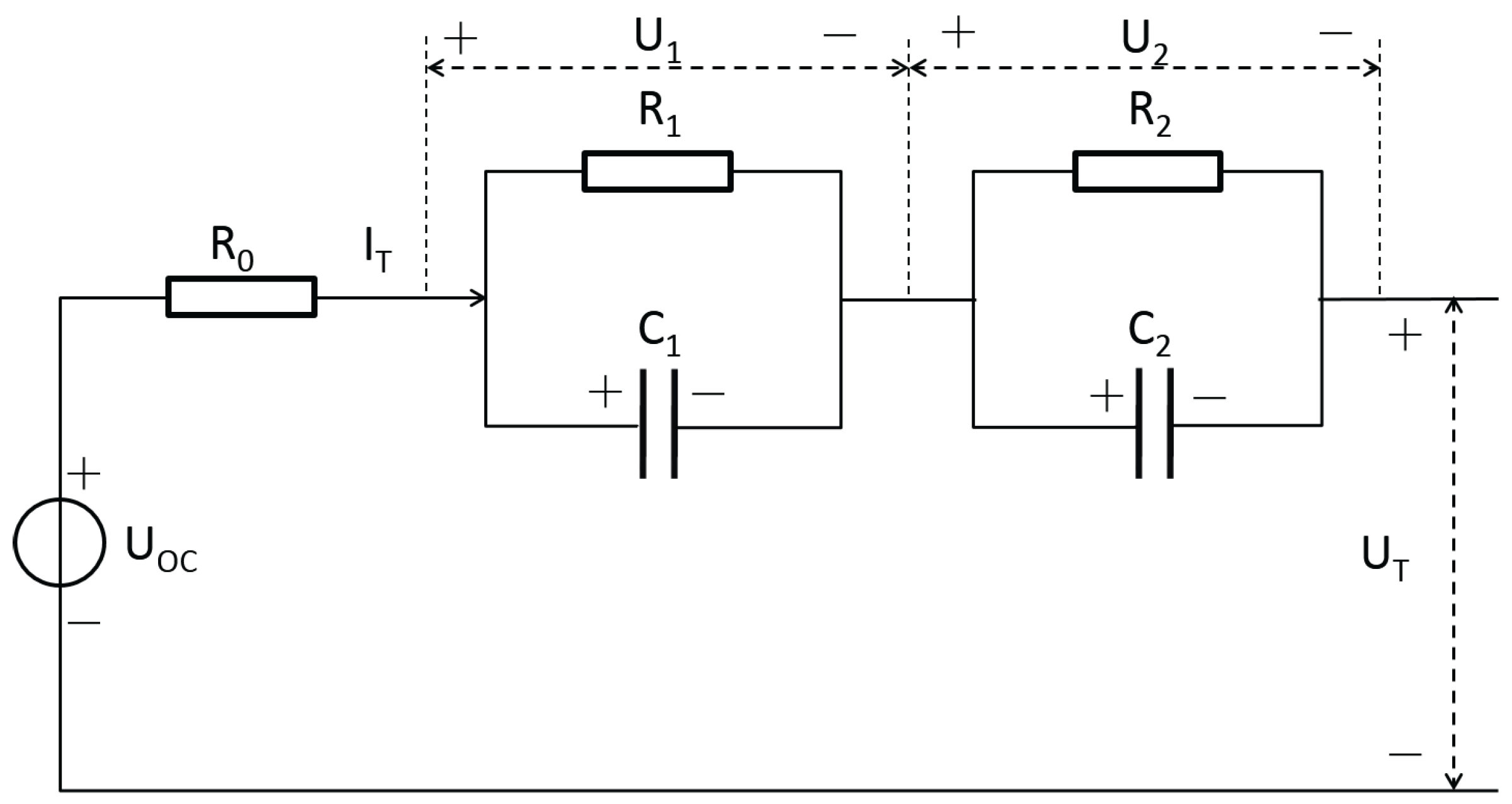
To accurately estimate the SOC of the battery packs in electrical vehicles, an accurate battery model is indispensable. Furthermore, for SOC estimation, the battery model should satisfy two essential requirements: (1) it can well capture the dynamic behaviors of the battery; (2) it should have a simple structure to easily establish the battery state-space equations and consume less computation of microcontrollers. As such, the second-order RC equivalent circuit model is employed here, and its schematic diagram is shown in Figure 1 [23,30].

In Figure 1, the notation $U_{OC}$ denotes the open-circuit voltage (OCV) related to SOC; $I_T$ is the operating current, which is positive in the discharge process and negative in the charge process; $U_T$ indicates the terminal voltage; and $R_0$ is Ohmic resistance. The notations $R_1$ and $C_1$ are the electrochemical polarization resistance and capacitance, respectively, and $R_2$ and $C_2$ are the concentration polarization resistance and capacitance, respectively. In addition, the voltages $U_1$ and $U_2$ denote the voltage of the electrochemical capacitors $C_1$ and concentration polarization capacitors $C_2$.

Now, let us establish the battery model. Based on the well-known Kirchhoff voltage laws, we have:

• State equation:

  $$\begin{array}{c}\hfill \left\{\begin{array}{cc}\hfill {\dot{U}}_1& =-\frac{1}{R_1{C}_1}{U}_1+\frac{1}{C_1}{I}_T\hfill \\ \hfill {\dot{U}}_2& =-\frac{1}{R_2{C}_2}{U}_2+\frac{1}{C_2}{I}_T\hfill \\ \hfill \dot{SOC}& =-\frac{1}{Q_n}{I}_T\hfill \end{array}\right.\end{array}$$

  (1)
• Output equation:

  $$\begin{array}{ccc}\hfill U_T& =& U_{OC}\left(SOC\right)-R_0{I}_T-U_1-U_2\hfill \end{array}$$

  (2)

where $Q_n$ is the nominal capacity of the battery.

3. Experiments and Identification of Model Parameters

In this section, the unknown parameters $R_0,R_1,R_2,C_1,C_2$ and nonlinear function $U_{OC}\left(SOC\right)$ in battery Equations (1) and (2) are identified by experiments [23,30]. First, let us introduce our test bench.

3.1. Test Bench

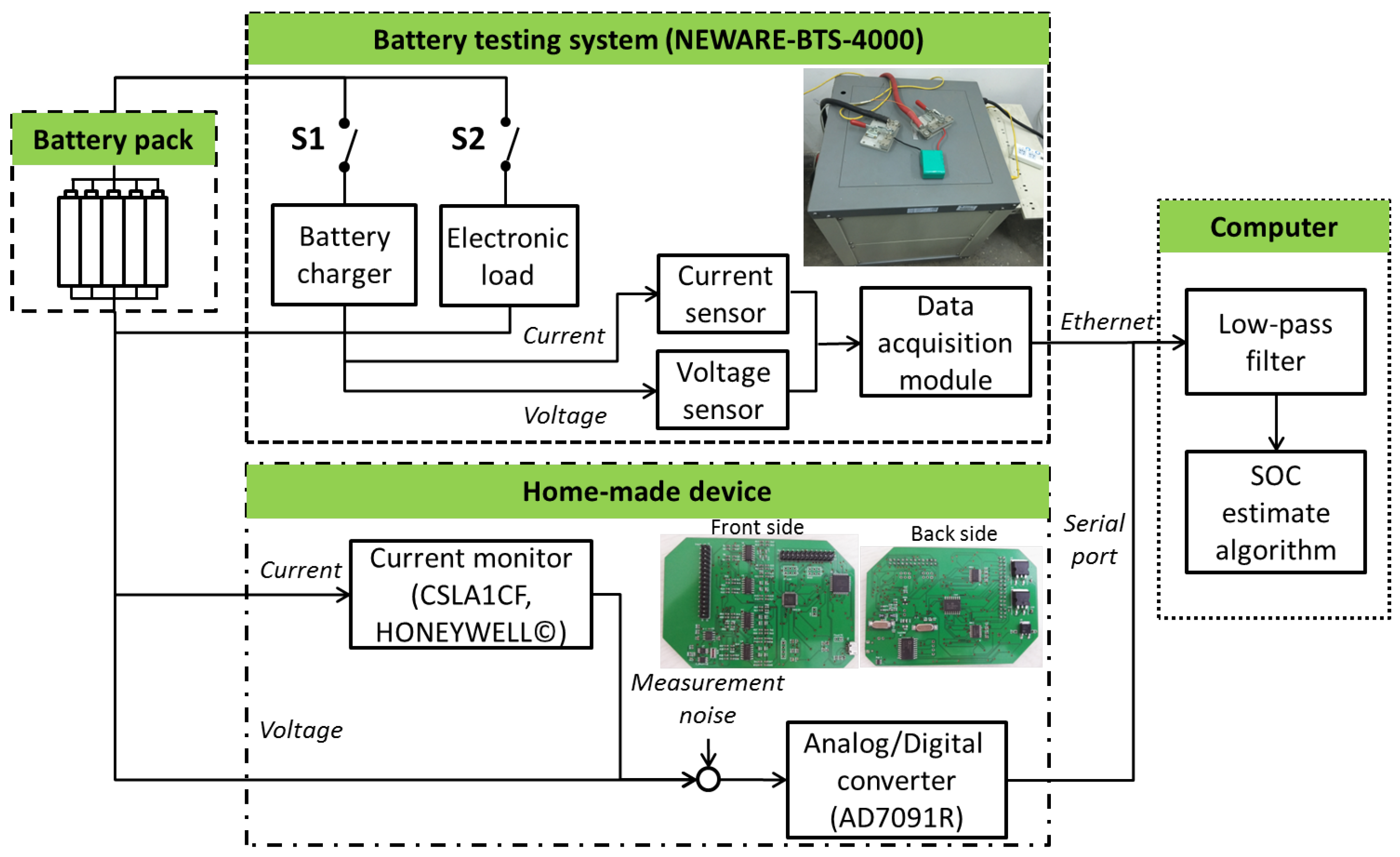
The established test bench shown in Figure 2 is utilized to test the characteristics of the battery, identify the parameters of the battery and verify the effectiveness of the proposed nonlinear observer-based SOC estimation method. The battery type used in the experiments is US18650GR-G7 manufactured by Sony Corporation, Tokyo Japan. Its nominal voltage is 3.7 V, and the nominal capacity is 2.4 Ah. Moreover, the test object is a battery pack with ten batteries connected in parallel. The standard current and voltage are measured by the the battery testing system BTS-4000 produced by NEWARE Electronic Co., Ltd., Shenzhen, China which are seen to have no measurement noise and used as the references of the terminal voltage and SOC. Meanwhile, a home-made current and voltage measurement device is also applied. The current and voltage measured by the home-made device have non-neglectable measurement noise due to the low cost and inaccurate current and voltage sensors, which is used to simulate the real measurement environment. It is worth noting that both the standard and home-made measurement data will be utilized to verify the effectiveness of the proposed SOC estimation methods. In Figure 2, the block diagram of the test bench is illustrated.

3.2. Parameters and Nonlinear Function Identification

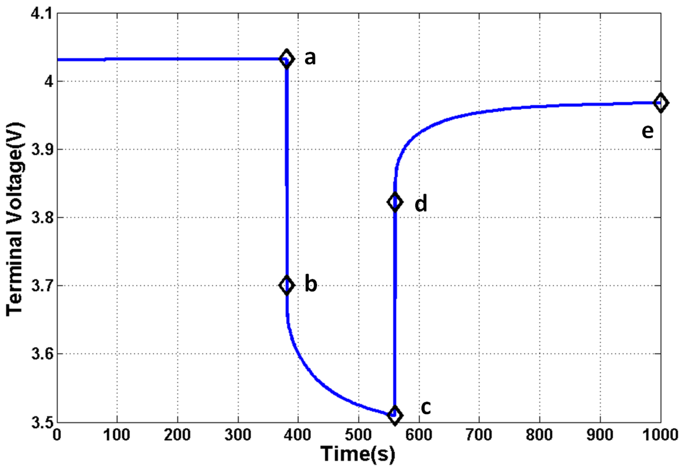
The principle of parameters identification depends on the physical behavior of the battery. In order to obtain accurate parameters, a typical discharging current profile is employed, and the corresponding terminal voltage profile is shown in Figure 3, where the battery stays on static before the experiment time $t\le t_a$, is discharged with 24 A between $t\in [t_a,t_c]$ and is in the relaxation process after $t\ge t_c$.

(1)

Identify parameter $R_0$: For the second-order RC model shown in the Figure 1, once the discharging/charging current is executed or stopped, the terminal voltage will drop or rise immediately. Notice that the voltages $U_1$ and $U_2$ of the capacitors $C_1$ and $C_2$ would not be suddenly changed at the moment of starting discharging/charging. Then, the ohmic resistance $R_0$ could be identified from variations of the terminal voltage at the moment of starting discharging/charging. As a consequence, the ohmic resistance $R_0$ can be calculated by:

$$\begin{array}{ccc}\hfill R_0& =& \frac{|V_T\left(t_b\right)-V_T\left(t_a\right)|+|V_T\left(t_d\right)-V_T\left(t_c\right)|}{2|I_T|}\hfill \end{array}$$

(3)

(2)

Identify parameters $R_1,R_2,C_1$ and $C_2$: The identification of the parameters $R_1$, $R_2$, $C_1$ and $C_2$ is divided into two steps. The fist step is to identify the time constants ${\tau }_1\triangleq R_1{C}_1$ and ${\tau }_2\triangleq R_2{C}_2$. Based on the identified time constants, the detailed identification of the $R_1$, $R_2$, $C_1$ and $C_2$ is introduced at another step. In addition, the response of the first-order RC circuit with the resistant R, capacitance C and constant current I is critical for the identification, which is given by:

$$\begin{array}{c}\hfill U\left(t\right)=U\left(t_0\right){\mathrm{e}}^{-\frac{t-t_0}{\tau }}+IR(1-{\mathrm{e}}^{-\frac{t-t_0}{\tau }})\end{array}$$

(4)

where $\tau =RC$ and $t_0$ is the initial time.

Step 1. Identify the time constants ${\tau }_1$ and ${\tau }_2$ during the relaxation process $c-d-e$: Note that the current equals zero during the relaxation process. Then, according to Equation (4), the voltages $U_1$ and $U_2$ can be calculated by:

$$\begin{array}{c}\hfill U_1\left(t\right)=U_1\left(t_c\right){\mathrm{e}}^{-\frac{t-t_c}{{\tau }_1}}\end{array}$$

(5)

$$\begin{array}{c}\hfill U_2\left(t\right)=U_2\left(t_c\right){\mathrm{e}}^{-\frac{t-t_c}{{\tau }_2}}\end{array}$$

(6)

respectively. From the output Equation (2), we have:

$$\begin{array}{c}\hfill U_T\left(t\right)=U_{OC}\left(SOC\right)-U_1\left(t_c\right){\mathrm{e}}^{-\frac{t-t_c}{{\tau }_1}}-U_2\left(t_c\right){\mathrm{e}}^{-\frac{t-t_c}{{\tau }_2}}\end{array}$$

which is rewritten as:

$$\begin{array}{c}\hfill U_T\left(t\right)={\alpha }_1-{\alpha }_2{\mathrm{e}}^{-\frac{t-t_c}{{\beta }_1}}-{\alpha }_3{\mathrm{e}}^{-\frac{t-t_c}{{\beta }_2}}\end{array}$$

(7)

where ${\alpha }_1,{\alpha }_2,{\alpha }_3,{\beta }_1,{\beta }_2$ are the unknown coefficients and will be identified later. Obviously, we see ${\alpha }_1=U_T(\infty )$ that is measured at the end of the relaxation process, i.e., the point e. By using the MATLAB function “Custom Equation” in the Curve Fitting Toolbox, the optimal coefficients ${\alpha }_2,{\alpha }_3,{\beta }_1,{\beta }_2$ can be obtained. Therefore, the time constants ${\tau }_1,{\tau }_2$ and the voltages $U_1\left(t_c\right),U_2\left(t_c\right)$ are identified.

Step 2: Identify parameters $R_1,C_1,R_2$ and $C_2$ during the discharging process $a-b-c$: Note that the point a is the end of the previous relaxation process. Then, we have $U_1\left(t_a\right)=0$ and $U_2\left(t_a\right)=0$. It follows from Equation (4) that:

$$\begin{array}{ccc}\hfill U_1\left(t\right)& =& I_T{R}_1(1-e^{-\frac{t-t_a}{{\tau }_1}})\hfill \end{array}$$

(8)

$$\begin{array}{ccc}\hfill U_2\left(t\right)& =& I_T{R}_2(1-e^{-\frac{t-t_a}{{\tau }_2}})\hfill \end{array}$$

(9)

Hence, the resistances $R_1,R_2$ are determined by the following equations:

$$\begin{array}{cc}\hfill R_1& =\frac{U_1\left(t_c\right)}{I_T\left(1-e^{-\frac{t_c-t_a}{{\tau }_1}}\right)}\end{array}$$

(10)

$$\begin{array}{cc}\hfill R_2& =\frac{U_2\left(t_c\right)}{I_T\left(1-e^{-\frac{t_c-t_a}{{\tau }_2}}\right)}\end{array}$$

(11)

where ${\tau }_1,{\tau }_2,U_1\left(t_c\right)$ and $U_2\left(t_c\right)$ have been calculated at the above Step 1. Since ${\tau }_1=R_1{C}_1,{\tau }_2=R_2{C}_2$, we can get $C_1=\frac{{\tau }_1}{R_1},C_2=\frac{{\tau }_2}{R_2}$. Therefore, the parameter identification is completed and shown in

Table 1. Identification result of the parameters.

${\mathit{R}}_0$	${\mathit{R}}_1$	${\mathit{R}}_2$	${\mathit{C}}_1$	${\mathit{C}}_2$
10.822 m$\mathrm{\Omega }$	3.103 m$\mathrm{\Omega }$	2.611 m$\mathrm{\Omega }$	8.4379 kF	91.401 kF

.

(3)

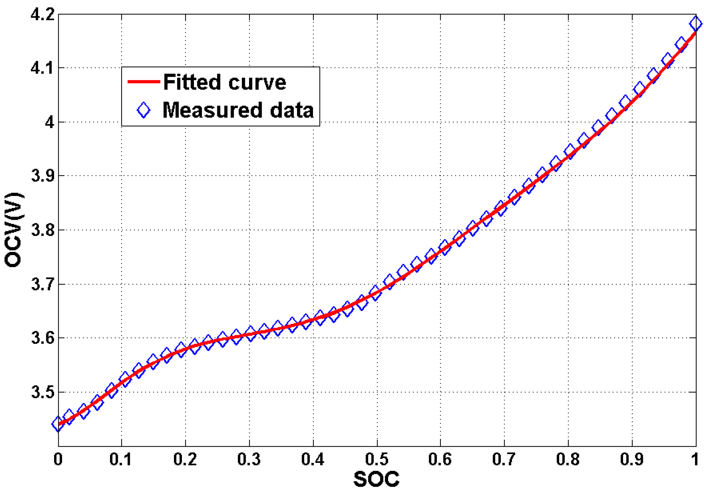
Identify the nonlinear function U${}_{OC}$(SOC): The curve fitting method is used to identify the nonlinear function U${}_{OC}$(SOC). Here, relatively accurate discharging experiments are carried out to reduce the fitting error of the curve fitting method, in which the discharging current pulse is set to be 24 A. The lasting time of the discharging current pulse is 72 s, which is utilized to achieve the 2% decline of SOC. Moreover, the battery is rest for 40 min after a discharging period to ensure the end of the relaxation process. In order to accurately fit the measurement data, the seventh-order polynomial is employed, which is given by:

$$\begin{array}{c}\hfill \begin{array}{ccc}\hfill U_{OC}\left(SOC\right)& =& -36.93SO{C}^7+142.4SO{C}^6-214.8SO{C}^5+158SO{C}^4\hfill \\ & & -56.25SO{C}^3+7.9SO{C}^2+0.4SOC+3.44\hfill \end{array}\end{array}$$

(12)

Finally, the validity of the above polynomial is shown in Figure 4.

3.3. Model Verification

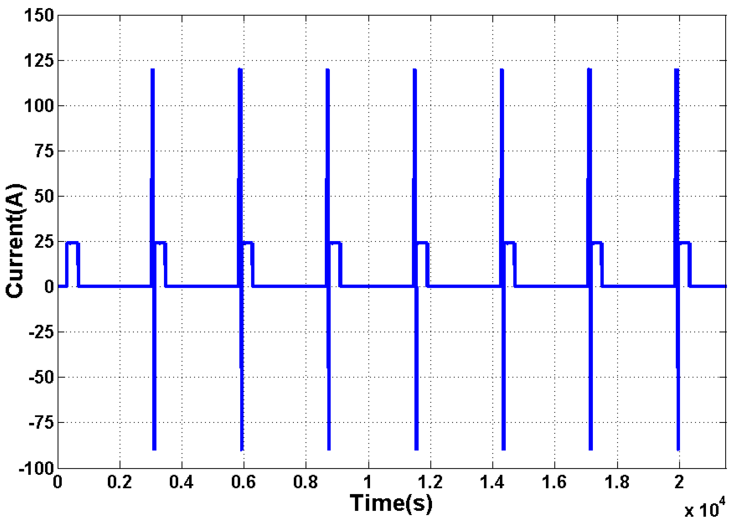
A typical Hybrid Pulse Power Characteristic (HPPC) test is adopted to prove the validity of battery Equations (1) and (2) with identified parameters in Table 1 and nonlinear Function (12). The test current is displayed in Figure 5, where the initial SOC is set to be 90%.

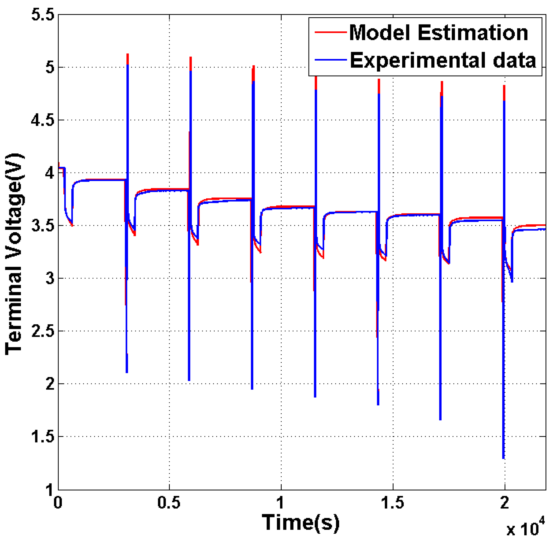
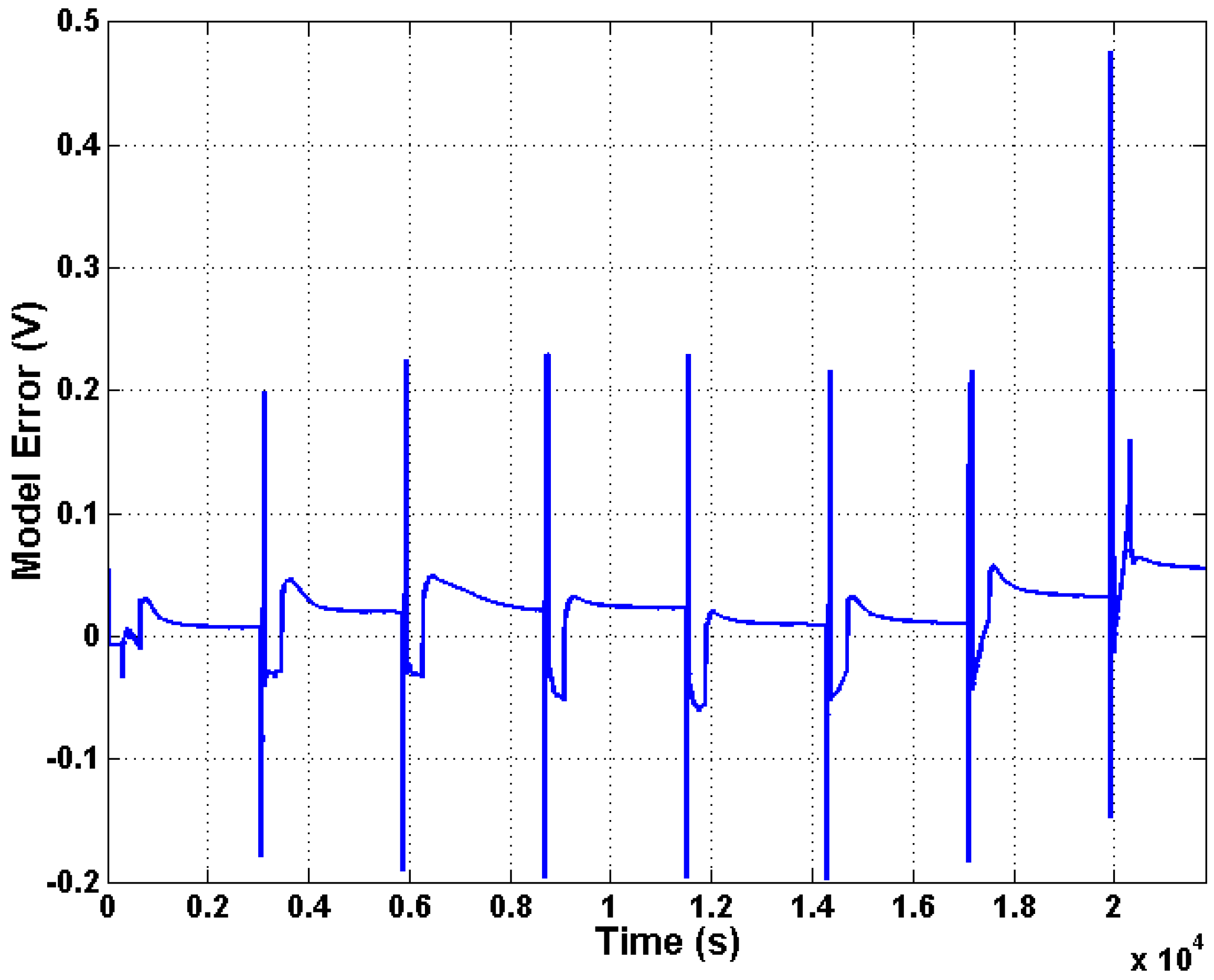
By calculating the output of battery Equations (1) and (2) with the parameters in Table 1, the modeling accuracy is shown in the following Figure 6 and Figure 7 and

Table 2. Modeling errors with respect to $U_T$.

Index	Maximum	Mean	Variance	Error Rate
Value	0.5562 V	0.0101 V	0.000706 ${\mathrm{V}}^2$	0.2733%

.

It is shown in Figure 6 that the identified model is almost coincident to the experimental data. Moreover, the model error in Figure 7 and Table 2 demonstrates the effectiveness of the identified model. From Table 2, we see that the parameters identification results and the identified second-order RC model are reasonable enough. Notice that the model parameters are identified from the first discharging process, i.e., the SOC range [80%, 90%]. Then, the model error of the first process is minimum among all eight processes. The second to the seventh processes denote the SOC range [20%, 80%]. In this range, the battery dynamics is similar, so these modeling errors are similar. The battery dynamics of the final process, i.e., the range [10%, 20%], is much different from the range [20%, 90%]. Therefore, the model error is greatly increased at the final discharging process.

Remark 1.

The parameters ($R_0/R_1/C_1/R_2/C_2$) are identified as constants, which is not true because of the effect of temperature and aging. However, due to the computation and the cost of the on-board battery management system considerations, the parameters need to be approximated as constants. Hence, one viable option is to update the parameters regularly by using off-line identification methods. Using the updated parameters, the proposed SOC estimation approach for constant parameters can ensure the accuracy of the SOC estimation.

4. Nonlinear Observer Design for SOC Estimation

The battery Equations (1) and (2) can be rewritten as the following nonlinear system:

$$\begin{array}{l}\hfill \left\{\begin{array}{l}\dot{\mathit{x}}=A\mathit{x}+Bu,\mathit{x}\left(0\right)={\mathit{x}}_0\\ y=h\left(\mathit{x}\right)+C\mathit{x}-R_{0}u\end{array}\right.\end{array}$$

(13)

where $\mathit{x}={[U_1,U_2,SOC]}^T,y=U_T,u=I_T$, $h\left(\mathit{x}\right)=U_{OC}\left(SOC\right)$, ${\mathit{x}}_0$ is the initial state and:

$$\begin{array}{c}\hfill A=\left[\begin{array}{ccc}-\frac{1}{{\tau }_1}& 0& 0\\ 0& -\frac{1}{{\tau }_2}& 0\\ 0& 0& 0\end{array}\right],B=\left[\begin{array}{c}\frac{1}{C_1}\\ \frac{1}{C_2}\\ -\frac{1}{Q_n}\end{array}\right],C^T=\left[\begin{array}{c}-1\\ -1\\ 0\end{array}\right]\end{array}$$

Since the battery charge-discharge process involves complicated physical and chemical reactions, the battery Equation (13) are further rewritten as:

$$\begin{array}{c}\hfill \left\{\begin{array}{l}\dot{\mathit{x}}=A\mathit{x}+Bu+{\omega }_x,\mathit{x}\left(0\right)={\mathit{x}}_0\\ y=h\left(\mathit{x}\right)+C\mathit{x}-R_{0}u+{\omega }_y\end{array}\right.\end{array}$$

(14)

where ${\omega }_x$ denotes the state disturbance that is the combination of the modeling error and measurement noise of the current and ${\omega }_y$ is the output disturbance that is the combination of the measurement noises of the current and terminal voltage. Notice that for the observer-based SOC estimate, the disturbances ${\omega }_x$ and ${\omega }_y$ are only assumed to be bounded, that is $\parallel {\omega }_x\parallel <\infty$ and $\parallel {\omega }_y\parallel <\infty$.

Let $\widehat{\mathit{x}}$ and $\widehat{SOC}$ be the estimates of the state $\mathit{x}$ and $SOC$, respectively, and $\tilde{h}\triangleq h\left(\mathit{x}\right)-h\left(\widehat{\mathit{x}}\right)$. Note that $SOC\in [0,1]$ and $U_{OC}\left(SOC\right)$ is a monotonically increasing function. Then, we have:

$$\begin{array}{c}\hfill {\beta }_{\min }\le {\dot{U}}_{OC}\left(SOC\right)\le {\beta }_{\max }\end{array}$$

(15)

with ${\beta }_{\min },{\beta }_{\max }>0$. Furthermore, from the SOC-OCV curve Equation (12), we have that the tested battery satisfies the above Equation (15) with:

$$\begin{array}{c}\hfill {\beta }_{\min }=0.2079,{\beta }_{\max }=1.4119\end{array}$$

(16)

To design the nonlinear observer of the above System Equation (14), the property of the nonlinear function $h\left(\mathit{x}\right)$ should be discussed firstly.

Property 1.

There exists matrix Q, such that the nonlinear functions $h\left(\mathit{x}\right)$ satisfies the following one-sided Lipschitz condition:

$$\begin{array}{c}\hfill -{\tilde{\mathit{x}}}^T{\left[\frac{\partial h}{\partial \mathit{x}}{|}_{\mathit{x}=\widehat{\mathit{x}}}\right]}^{\mathrm{T}}\tilde{h}\le -{\tilde{\mathit{x}}}^{T}Q\tilde{\mathit{x}}\end{array}$$

(17)

for any $\mathit{x},\widehat{\mathit{x}}$ with $SOC,\widehat{SOC}\in [0,1]$, where:

$$\begin{array}{c}\hfill Q=\left[\begin{array}{ccc}0& 0& 0\\ 0& 0& 0\\ 0& 0& {\beta }_{\min }^2\end{array}\right]\end{array}$$

(18)

Proof. 

By utilizing the mean value theorem, we have:

$$\begin{array}{c}\hfill \tilde{h}=h\left(\mathit{x}\right)-h\left(\widehat{\mathit{x}}\right)=\frac{\partial h}{\partial \mathit{x}}{|}_{\mathit{x}=\zeta }(\mathit{x}-\widehat{\mathit{x}})\end{array}$$

(19)

where $\mathit{\zeta }\triangleq {[{\mathit{\zeta }}_{U_1},{\mathit{\zeta }}_{U_2},{\mathit{\zeta }}_{SOC}]}^{\mathrm{T}}\in [\mathit{x},\widehat{\mathit{x}}]$ Note that:

$$\begin{array}{c}\hfill \frac{\partial h}{\partial \mathit{x}}=\left[\frac{\partial h\left(\mathit{x}\right)}{\partial U_1},\frac{\partial h\left(\mathit{x}\right)}{\partial U_2},\frac{\partial h\left(\mathit{x}\right)}{\partial SOC}\right]=[0,0,{\dot{U}}_{OC}\left(SOC\right)]\end{array}$$

Then, we have:

$$\begin{array}{c}\hfill \begin{array}{c}-{\tilde{\mathit{x}}}^{\mathrm{T}}{\left[\frac{\partial h}{\partial \mathit{x}}{|}_{\mathit{x}=\widehat{\mathit{x}}}\right]}^{\mathrm{T}}\tilde{h}=-{\tilde{\mathit{x}}}^{\mathrm{T}}{\left[\begin{array}{ccc}0& 0& {\dot{U}}_{OC}(\widehat{SOC})\end{array}\right]}^{\mathrm{T}}\tilde{h}\hfill \\ =-{\dot{U}}_{OC}(\widehat{SOC})·\widetilde{SOC}·\tilde{h}\hfill \\ \le -{\beta }_{\min }·\widetilde{SOC}·\tilde{h}\hfill \\ =-{\beta }_{\min }\left({\tilde{\mathit{x}}}^{\mathrm{T}}{\left[0,0,1\right]}^{\mathrm{T}}\right)([0,0,{\dot{U}}_{OC}\left({\mathit{\zeta }}_{SOC}\right)]\tilde{\mathit{x}})\hfill \\ \le -{\tilde{\mathit{x}}}^{\mathrm{T}}\left[\begin{array}{ccc}0& 0& 0\\ 0& 0& 0\\ 0& 0& {\beta }_{\min }^2\end{array}\right]\tilde{\mathit{x}}\hfill \end{array}\end{array}$$

(20)

This implies that Condition Equation (17) with Equation (18) holds. The proof is completed. ☐

Remark 2.

Condition Equation (17) is one-sided Lipschitz condition Equation [34] with respect to ${\left[\frac{\partial h}{\partial \mathit{x}}{|}_{\mathit{x}=\widehat{\mathit{x}}}\right]}^{\mathrm{T}}\tilde{h}$, which plays an important role in the observer design. Compared with the classic Lipschitz condition (e.g., ${\tilde{h}}^{\mathrm{T}}\tilde{h}\le \beta {\widehat{\mathit{x}}}^{\mathrm{T}}\widehat{\mathit{x}},\beta >0$), the one-sided Lipschitz Condition Equation (17) can make the nonlinear function $h\left(\mathit{x}\right)$ contribute to the observer design due to the positive semi-definite matrix Q. Note that $(A,C)$ is not observable. Thus, the nonlinear function $h\left(\mathit{x}\right)$ must play a positive role for the observer design. This is the main reason to establish the one-sided Lipschitz Condition Equation (17).

Next, let us design the nonlinear observer as follows:

$$\begin{array}{c}\hfill \left\{\begin{array}{ccc}\hfill \dot{\widehat{\mathit{x}}}& =& A\widehat{\mathit{x}}+Bu+L{\left[\frac{\partial h}{\partial \mathit{x}}\right]}_{\mathit{x}=\widehat{\mathit{x}}}^T(y-\widehat{y}),\widehat{\mathit{x}}\left(0\right)={\widehat{\mathit{x}}}_0\hfill \\ \hfill \widehat{y}& =& h\left(\widehat{\mathit{x}}\right)+C\widehat{\mathit{x}}-R_{0}u\hfill \end{array}\right.\end{array}$$

(21)

where $\widehat{y}$ is the estimate of the real terminal voltage y, L is the matrix that will be designed later, but the vector $L{\left[\frac{\partial h}{\partial \mathit{x}}\right]}_{\mathit{x}=\widehat{\mathit{x}}}^T$ is the actual observer gain that is dynamic. It follows that the error dynamics is given by:

$$\begin{array}{c}\hfill \begin{array}{ccc}\hfill \dot{\tilde{\mathit{x}}}& =& \left(A-L{\left[\frac{\partial h}{\partial \mathit{x}}\right]}_{\mathit{x}=\widehat{\mathit{x}}}^{T}C\right)\tilde{\mathit{x}}-L{\left[\frac{\partial h}{\partial \mathit{x}}\right]}_{\mathit{x}=\widehat{\mathit{x}}}^T\tilde{h}+(E-L{\left[\frac{\partial h}{\partial \mathit{x}}\right]}_{\mathit{x}=\widehat{\mathit{x}}}^{T}F)\mathit{\omega }\hfill \end{array}\end{array}$$

(22)

where $\tilde{\mathit{x}}=\mathit{x}-\widehat{\mathit{x}}$ is the estimate error of the state, $\mathit{\omega }=\left[\begin{array}{c}{\omega }_x\\ {\omega }_y\end{array}\right]$ the synthetic disturbance, $E=[I_0,0],F=[0,1]$ and $I_0$ denotes the appropriate dimensional identity matrix.

Now, let us establish the following nonlinear observer design criterion with an $H_{\infty }$ performance, which is the main contribution of this paper.

Theorem 1.

For given positive scalars $ϵ<2{\beta }_{\min }^2$ and γ, if there exist matrix $P=P^{\mathrm{T}}>0$ and vector S, such that the following LMIs:

$$\begin{array}{c}\hfill \left\{\begin{array}{c}\mathrm{\Pi }=\left[\begin{array}{cc}{\mathrm{\Pi }}_{11}& PE-R_{1}SF\\ *& -{\gamma }^2{I}_0\end{array}\right]<0\\ R_{2}S<{\beta }_{max}\\ R_{2}S>{\beta }_{min}\end{array}\right.\end{array}$$

(23)

where ${\mathrm{\Pi }}_{11}=PA+A^{\mathrm{T}}P-R_{1}SC-C^{\mathrm{T}}{S}^{\mathrm{T}}{R}_1^{\mathrm{T}}+ϵI_0-2Q$, $R_1=\left[\begin{array}{ccc}0& 0& 0\\ 0& 0& 0\\ 0& 0& 1\end{array}\right]$, $R_2={\left[\begin{array}{c}0\\ 0\\ 1\end{array}\right]}^{\mathrm{T}}$, then the battery Equation (14) and the nonlinear observer Equation (21) $L=P^{-1}$ satisfy the $H_{\infty }$ performance with the given attenuation $\gamma >0$, that is:

$$\begin{array}{ccc}\hfill {\int }_{t=0}^{\mathrm{\Gamma }}{\parallel \tilde{\mathit{x}}\left(t\right)\parallel }^2\mathrm{d}t& <& {\lambda }_{max}\left(P\right)\parallel \tilde{\mathit{x}}{\left(0\right)\parallel }^2+\frac{{\gamma }^2}{ϵ}{\int }_0^{\mathrm{\Gamma }}{\parallel \mathit{\omega }\left(t\right)\parallel }^2\mathrm{d}t\hfill \end{array}$$

for any $\mathrm{\Gamma }>0$.

Proof. 

Let the candidate of the Lyapunov function be:

$$\begin{array}{c}\hfill V\left(\tilde{\mathit{x}}\right)={\tilde{\mathit{x}}}^{\mathrm{T}}P\tilde{\mathit{x}}\end{array}$$

(24)

and the observer gain $L=P^{-1}$. Then, the derivative of $V\left(\tilde{\mathit{x}}\right)$ along the trajectories of the error System Equation (22) yields:

$$\begin{array}{ccc}\hfill \dot{V}\left(\tilde{\mathit{x}}\right)& =& 2{\tilde{\mathit{x}}}^T\left[(PA-{\left[\frac{\partial h}{\partial \mathit{x}}\right]}_{\mathit{x}=\widehat{\mathit{x}}}^{T}C)\tilde{\mathit{x}}-{\left[\frac{\partial h}{\partial \mathit{x}}\right]}_{\mathit{x}=\widehat{\mathit{x}}}^{\mathrm{T}}\tilde{h}+(PE-{\left[\frac{\partial h}{\partial \mathit{x}}\right]}_{\mathit{x}=\widehat{\mathit{x}}}^{\mathrm{T}}F)\mathit{\omega }\right]\hfill \end{array}$$

Note that ${\left[\frac{\partial h}{\partial \mathit{x}}\right]}_{\mathit{x}=\widehat{\mathit{x}}}^{\mathrm{T}}=[0,0,{\dot{U}}_{OC}(\widehat{SOC})]$, ${\beta }_{\min }\le {\dot{U}}_{OC}\left(SOC\right)\le {\beta }_{\max }$ and the one-sided Lipschitz Condition Equation (17). Then, the derivative $\dot{V}\left(\tilde{\mathit{x}}\right)$ can be rewritten as:

$$\begin{array}{c}\hfill \dot{V}\left(\tilde{\mathit{x}}\right)=2{\tilde{\mathit{x}}}^T[(PA-R_{1}SC-Q)\tilde{\mathit{x}}+(PE-R_{1}SF)\mathit{\omega }]\end{array}$$

(25)

where $S\triangleq {[s_1,s_2,s_3]}^{\mathrm{T}}$ is a vector satisfying ${\beta }_{\min }\le R_{2}S=s_3\le {\beta }_{\max }$.

To establish the $H_{\infty }$ performance, we introduce the performance index:

$$\begin{array}{c}\hfill J\left(t\right)=\dot{V}\left(\tilde{\mathit{x}}\right)+ϵ{\tilde{\mathit{x}}}^{\mathrm{T}}\tilde{\mathit{x}}-{\gamma }^2{\mathit{\omega }}^{\mathrm{T}}\mathit{\omega }\end{array}$$

(26)

where $ϵ<2{\beta }_{\min }^2$ is used to guarantee that the matrix ${\mathrm{\Pi }}_{11}$ could be negative definite. It follows that:

$$\begin{array}{c}\hfill J\left(t\right)={\left[\begin{array}{c}\tilde{\mathit{x}}\\ \mathit{\omega }\end{array}\right]}^{\mathrm{T}}\mathrm{\Pi }\left[\begin{array}{c}\tilde{\mathit{x}}\\ \mathit{\omega }\end{array}\right]\end{array}$$

(27)

where $\mathrm{\Pi }$ is defined by Equation (23). Hence, we see that:

$$\begin{array}{c}\hfill \mathrm{\Pi }<0,R_{2}S<{\beta }_{max},R_{2}S>{\beta }_{min}\end{array}$$

(28)

can ensure $J\left(t\right)<0$. Note that ${\int }_0^{\mathrm{\Gamma }}\dot{V}\left(\tilde{\mathit{x}}\right)\mathrm{d}t=V\left(\mathrm{\Gamma }\right)-V\left(0\right)\ge -V\left(0\right)\ge -{\lambda }_{\max }\left(P\right){\parallel \tilde{\mathit{x}}\left(0\right)\parallel }^2$. Therefore, we have ${\int }_0^{\mathrm{\Gamma }}{\tilde{\mathit{x}}}^{\mathrm{T}}\tilde{\mathit{x}}\mathrm{d}t\le \frac{{\lambda }_{\max }\left(P\right)}{ϵ}{\parallel \tilde{\mathit{x}}\left(0\right)\parallel }^2+\frac{{\gamma }^2}{ϵ}{\int }_0^{\mathrm{\Gamma }}{\mathit{\omega }}^{\mathrm{T}}\mathit{\omega }\mathrm{d}t$ for any $\mathrm{\Gamma }>0$. The proof is completed. ☐

Remark 3.

The nonlinear observer design criterion Equation (23) is represented as the form of LMIs that is easily solved by the LMI MATLAB Toolbox [33]. Here, employing the vector S is critical to use the LMI to deal with the nonlinear function ${\left[\frac{\partial h}{\partial \mathit{x}}\right]}_{\mathit{x}=\widehat{\mathit{x}}}^{\mathrm{T}}$. Notice that the disturbance ω includes the measurement noise and the modeling error. The upper bound of disturbance ω is different and difficult to be accurately estimated for different operation conditions with various static and dynamic charging/discharging currents. However, the existing works usually utilized the upper bound of the disturbance ω to calculate the observer gain to ensure the convergence [23,24,26,30]. Hence, the observer designed in [23,24,26,30] may not be the optimal one to estimate the SOC. Oppositely, the proposed nonlinear observer by calculating the LMIs Equation (23) does not depend on the estimation of the disturbance ω, which makes the calculated observer suitable for various operating conditions.

5. Experimental Validations of the SOC Estimation

By utilizing the feasp function in LMI MATLAB Toolbox to solve the observer design criterion Equation (23), the matrix L in Equation (21) is calculated by:

$$\begin{array}{c}\hfill L=\left[\begin{array}{ccc}2.53\times {10}^{-5}& 7.56\times {10}^8& 2.56\times {10}^{-5}\\ 7.56\times {10}^{-8}& 0.00023& 0.0023\\ 2.56\times {10}^{-5}& 0.0023& 0.536\end{array}\right]\end{array}$$

(29)

In this section, the efficiency of the proposed nonlinear observer Equation (21) with gain Equation (29) will be verified by both the static and dynamic experimental operating conditions. Furthermore, in order to show the advantages of the proposed nonlinear observer design criterion, the classic EKF is also employed. It should be noted that in the following figures, the lines named as “Reference” are directly obtained by the standard measurement data, and the other lines are calculated by the home-made measurement data.

5.1. Static Experimental Validation

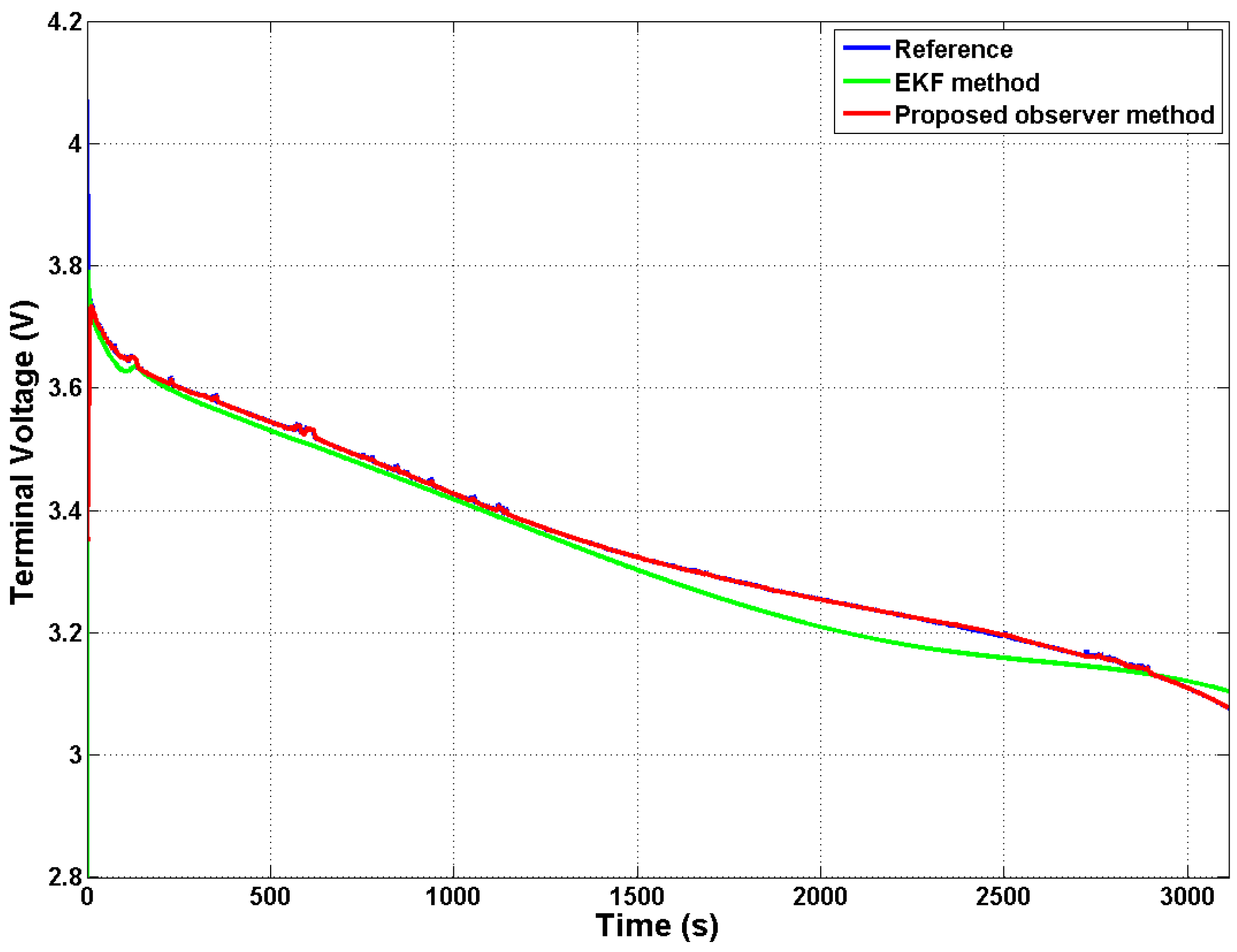
In this experiment, the discharging current is set to constant 24 A in the battery testing system. The proposed method is compared with the widely-used EKF method in terms of the terminal voltage estimation $\widehat{y}$ and its errors in Figure 8 and Figure 9. Meanwhile, SOC estimation $\widehat{SOC}$ and its errors are shown in Figure 10 and Figure 11, respectively. Moreover, the error distribution is shown in Figure 12.

5.2. Dynamic Experimental Validation

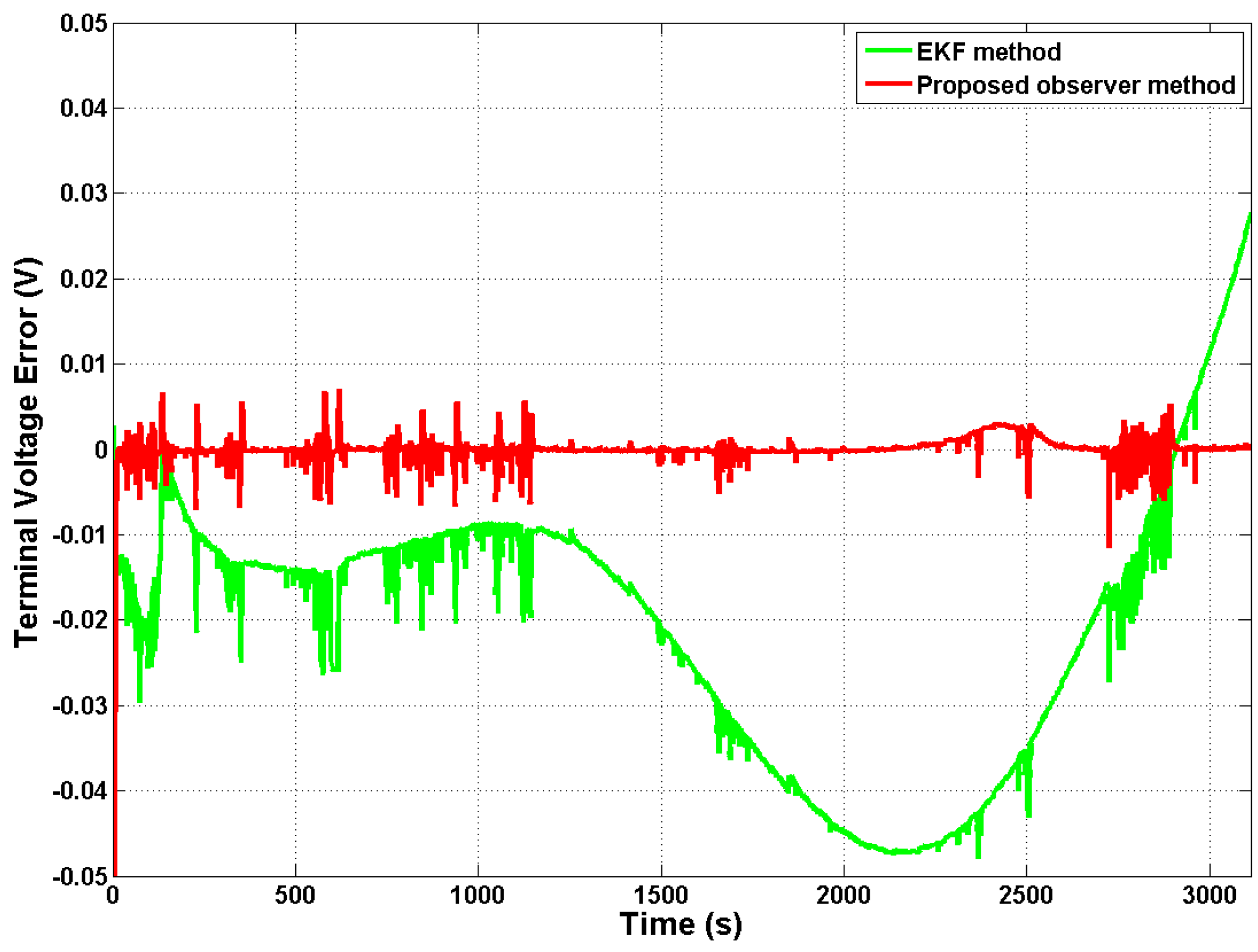
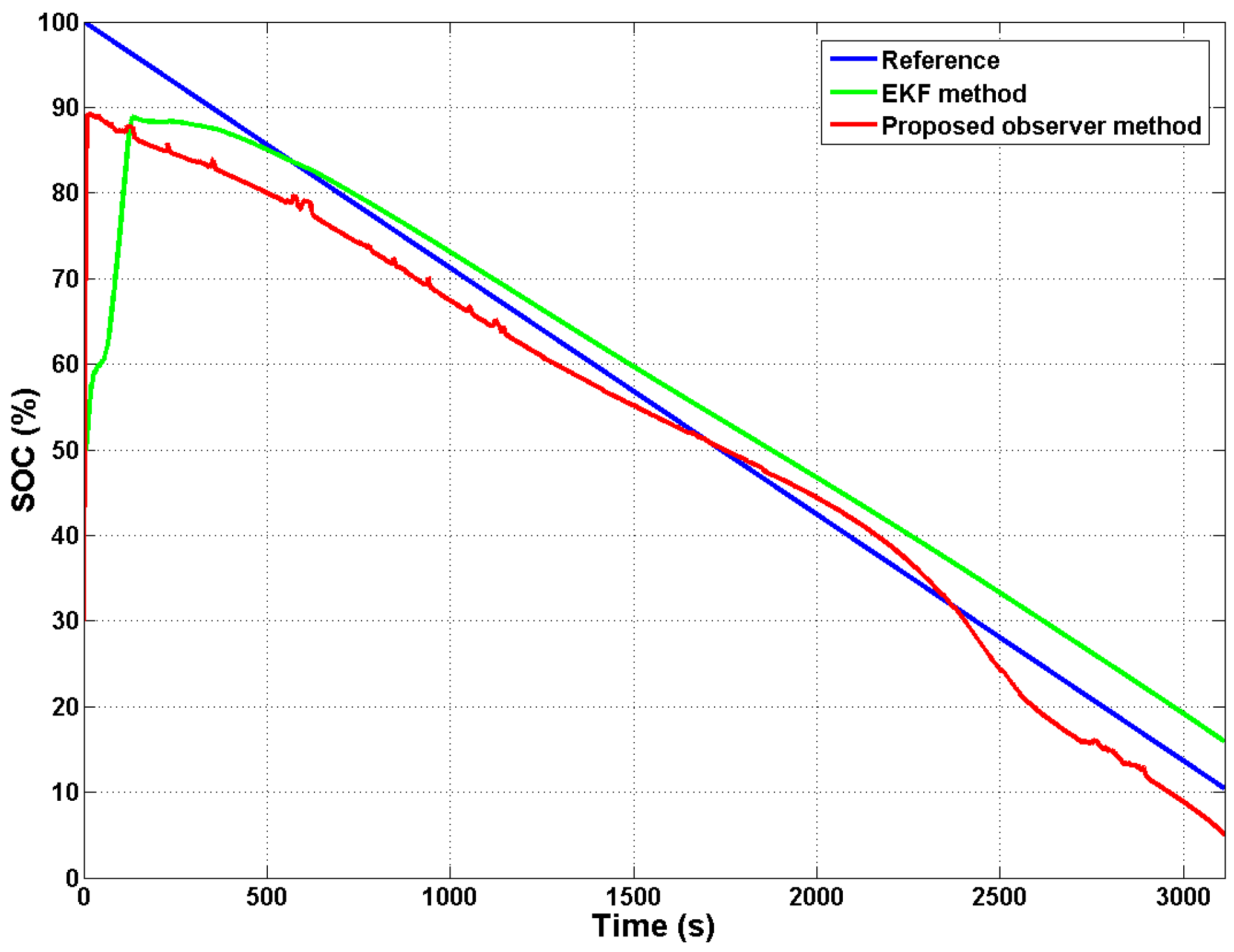
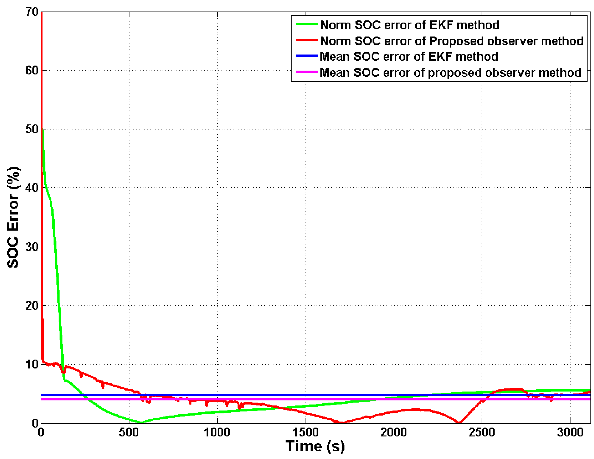
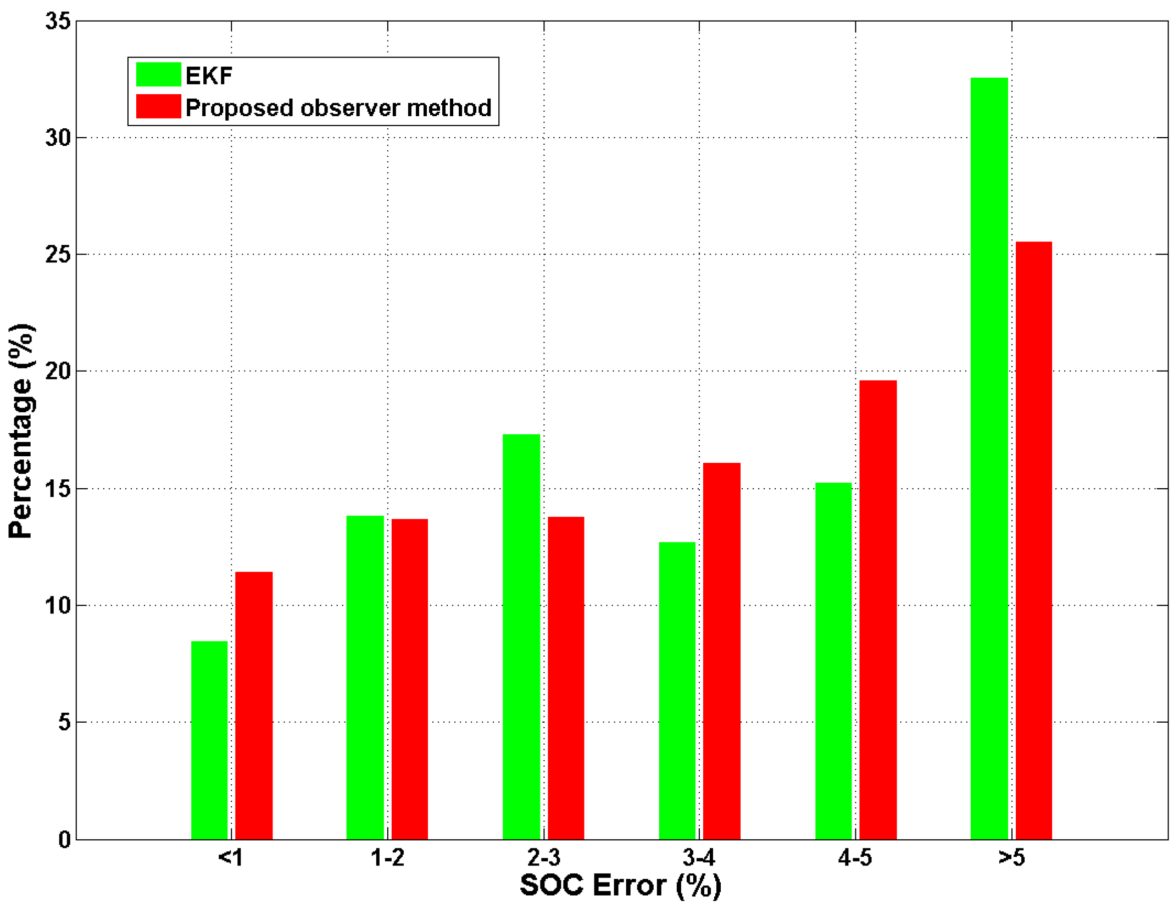
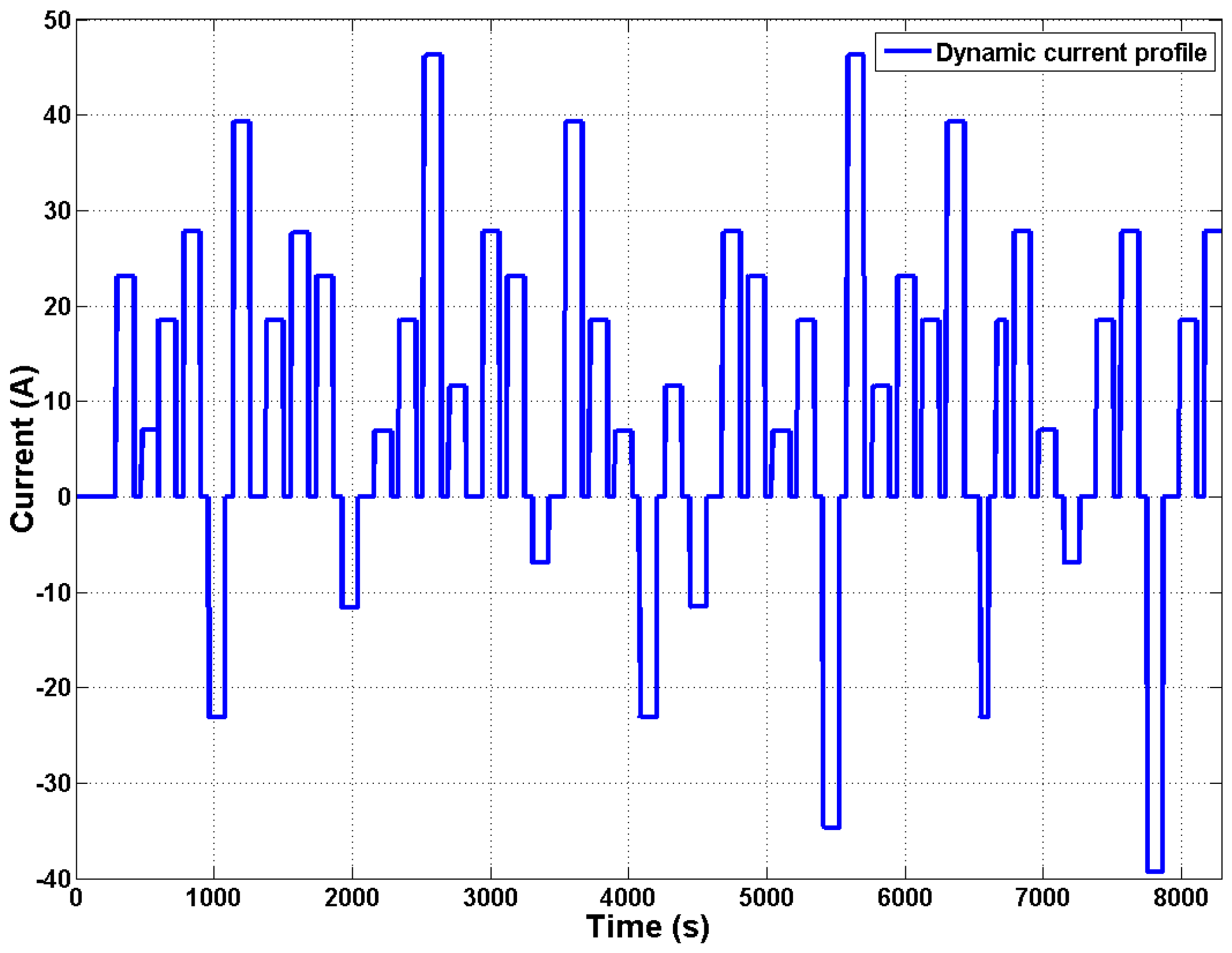
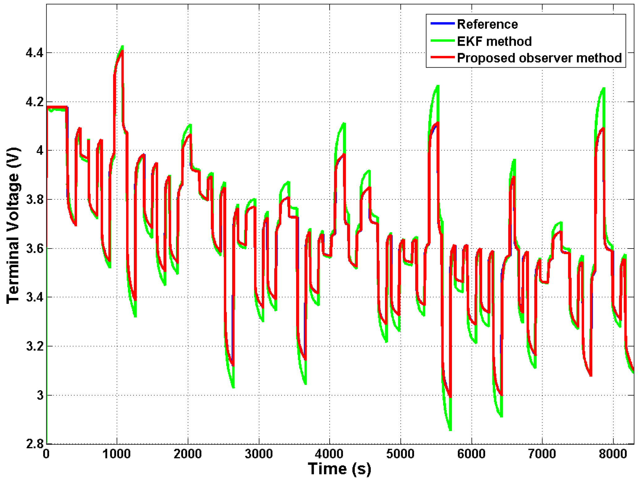
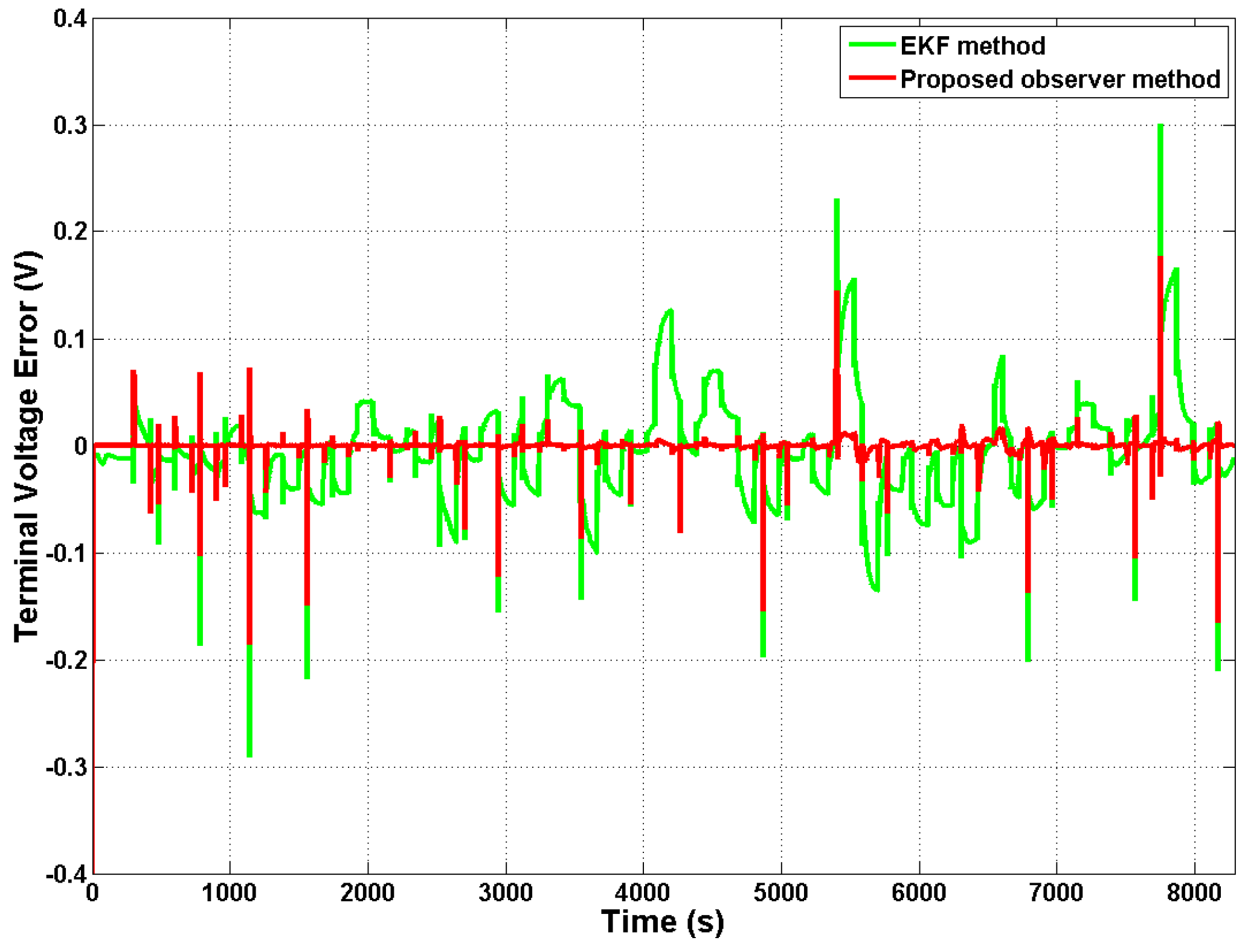
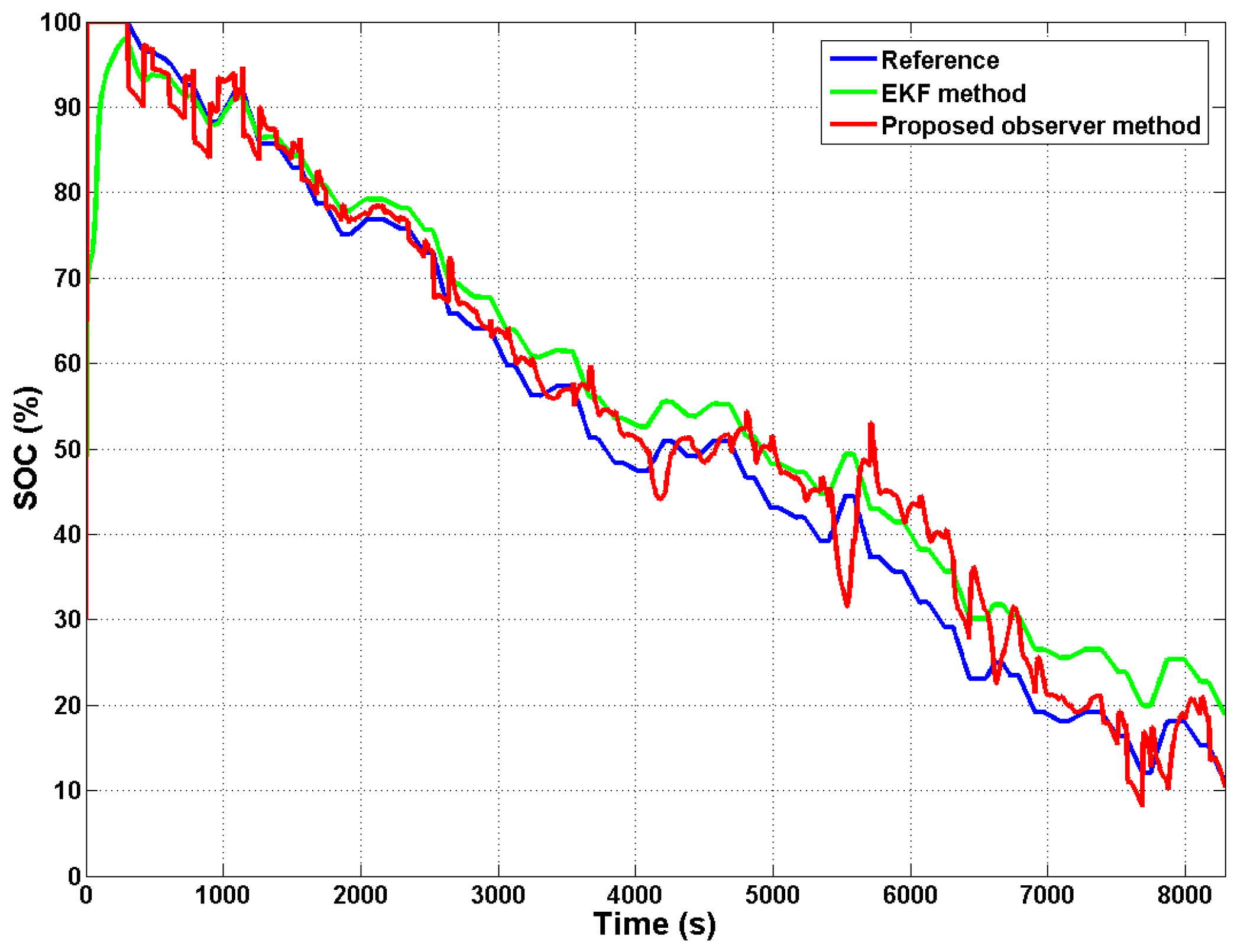
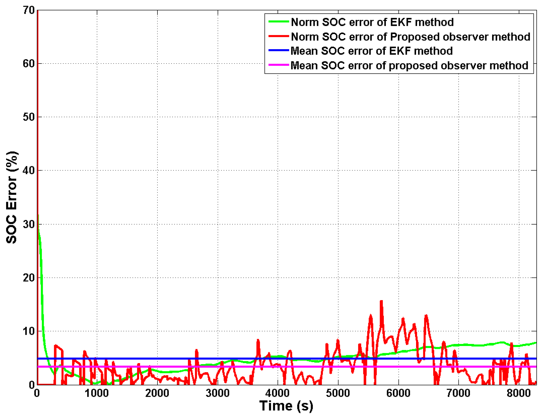
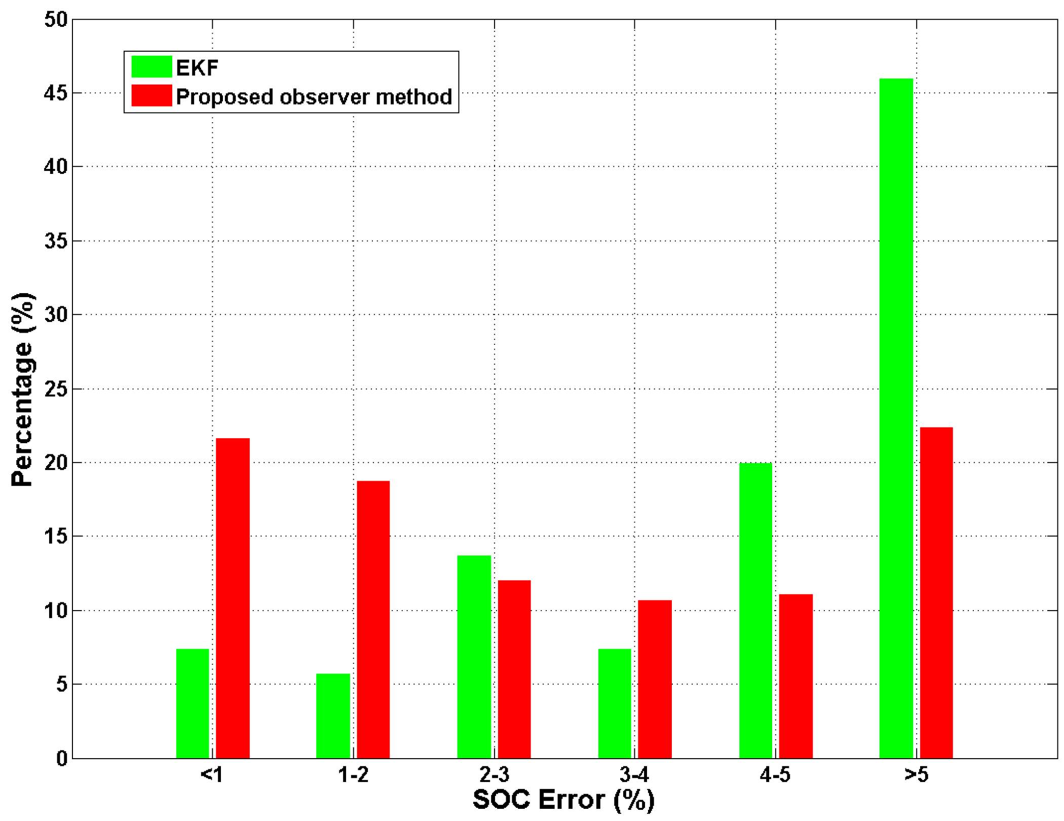
To evaluate the performance of the proposed SOC estimation method against EKF further, a dynamic current profile is applied in Figure 13. The difference between the dynamic experiment and the static experiment is that discharging current changes rapidly every one or two minutes. The measurement and estimations of terminal voltage and its errors are shown in Figure 14 and Figure 15. The measurement and estimations of SOC and its errors are also shown in Figure 16 and Figure 17. A comparison of the mean SOC estimation error between the EKF method and the proposed observer method can be seen in

Table 3. Comparison of mean SOC estimation error between the EKF method and the proposed observer method.

Experiment	Static Experiment	Dynamic Experiment
EKF	$4.71\%$	4.86%
Proposed observer	3.96%	3.36%

.

It is shown in Figure 8, Figure 9, Figure 14 and Figure 15 that the terminal voltage estimation of the proposed nonlinear observer is much better than that of the EKF. To some extent, this is the main reason why the SOC estimation of the the proposed nonlinear observer is better than that of the EKF, which is demonstrated in Figure 11, Figure 12, Figure 17, Figure 18 and Table 3. It is noteworthy that compared with the dynamic case, the proposed nonlinear observer is not much better than the EKF for the static case. Compared with the EKF, the main advantage of the nonlinear observer is the ability to quickly adjust the state estimate when facing the dramatic change in the output. For the static case, the change of the measurement output is slow, which implies that the advantage of the nonlinear observer is not well stimulated.

5.3. SOC Estimation Results and Evaluation

The following results can be derived from the above two experiments:

• From Figure 8, Figure 9, Figure 14 and Figure 15, we come to the conclusion that the terminal voltage estimation error of the proposed observer is much smaller than that of the EKF. It is shown in Figure 16 that the SOC estimation profile of the EKF is smoother than that of the proposed observer. The main reason for the above two situations is that the observer-based method pays more attention to the accuracy of the output estimation than the filter-based method.
• It is shown in Figure 10, Figure 11, Figure 16 and Figure 17 that the convergence rate of the proposed observer is much faster than that of the EKF. The error distributions shown in Figure 12 and Figure 18 indicate that the percentage bar of small SOC estimation error of the proposed observer is higher than that of the EKF. In addition, the mean SOC estimation errors in Table 3 clearly demonstrate that the proposed observer outperforms the EKF in both the static and dynamic experiments.
• The $H_{\infty }$ performance of the proposed nonlinear observer is the main reason why the proposed observer is superior to the EKF. Notice that the modeling error rather than the measurement noises is the main factor affecting the SOC estimation [4]. Furthermore, the modeling error is non-Gaussian. Thus, by using the $H_{\infty }$ method to restrict the effect of the modeling error on the state estimation, the SOC estimation of the $H_{\infty }$ observer is better than that of EKF.

Considering the above analysis, we can see that the proposed observer SOC estimation method is effective and has higher accuracy than the EKF method. The proposed method can be performed online and can estimate terminal voltage and SOC accurately and reliably. Meanwhile, the proposed method exhibits satisfying performance, especially considering the simplicity and feasibility of the battery model in real applications.

6. Conclusions

In this paper, a nonlinear observer with time-varying gain algorithm is presented to accurately estimate the SOC of the lithium-ion batteries in electric vehicles. The commonly-used second-order RC model is applied to simulate the nonlinear behaviors of the lithium-ion battery. The OCV-SOC relationship is fitted using the seventh-order polynomial, and the other RC parameters of the battery model are determined by the physical behavior of the battery. The principle of the nonlinear observer algorithm for battery SOC estimation is to introduce the $H_{\infty }$ performance to reduce the effect of the non-Gaussian system and measurement noises, which cannot be well filtered by EKF. Both the static and dynamic experiments are applied to assess the performance of the proposed method by comparing with the traditional EKF algorithms. Experimental results indicate that the proposed observer algorithm is helpful to improve the SOC estimation accuracy.

Notably, the parameters ($R_0/R_1/C_1/R_2/C_2$) are assumed to be constants, which may affect the practicability of the proposed approach due to the temperature and aging. To improve the SOC estimation accuracy, ongoing research is towards the iterative learning-based off-line identification method that could accurately identify the parameters related to the temperature and SOC.

References

- Eshani, M.; Gao, Y.; Gay, S.E.; Emadi, A. Modern Electric, Hybrid Electric, and Fuel Cell Vehicles; CRC Press: Boca Raton, FL, USA, 2005. [Google Scholar]
- He, H.; Xiong, R.; Zhang, X.; Sun, F.; Fan, J. State-of-Charge Estimation of the Lithium-Ion Battery Using an Adaptive Extended Kalman Filter Based on an Improved Thevenin Model. IEEE Trans. Veh. Technol. 2011, 60, 1461–1469. [Google Scholar]
- Cheng, K.W.E.; Divakar, B.P.; Wu, H.; Ding, K.; Ho, H.F. Battery-management system (BMS) and SOC development for electrical vehicles. IEEE Trans. Veh. Technol. 2011, 60, 76–88. [Google Scholar] [CrossRef]
- Waag, W.; Fleischer, C.; Sauer, D.U. Critical review of the methods for monitoring of lithium-ion batteries in electric and hybrid vehicles. J. Power Sources 2014, 258, 321–339. [Google Scholar] [CrossRef]
- Grewal, M.S.; Andrews, A.P. Kalman Filtering Theory and Practice Using Matlab, 4th ed.; John Wiley & Sons, Inc.: Hoboken, NJ, USA, 2015. [Google Scholar]
- Smith, K.A.; Rahn, C.D.; Wang, C.Y. Model-based electrochemical estimation and constraint management for pulse operation of lithium ion batteries. IEEE Trans. Control Syst. Technol. 2010, 18, 654–663. [Google Scholar] [CrossRef]
- Charkhgard, M.; Farrokhi, M. State-of-Charge Estimation for Lithium-Ion Batteries Using Neural Networks and EKF. IEEE Trans. Ind. Electron. 2010, 57, 4178–4187. [Google Scholar] [CrossRef]
- Shahriari, M.; Farrokhi, M. On-line State of Health Estimation of VRLA Batteries Using State of Charge. IEEE Trans. Ind. Electron. 2012, 60, 191–202. [Google Scholar] [CrossRef]
- Watrin, N.; Roche, R.; Ostermann, H.; Blunier, B.; Miraoui, A. Multiphysical lithium-based battery model for use in state-of-charge determination. IEEE Trans. Veh. Technol. 2012, 60, 3420–3429. [Google Scholar] [CrossRef]
- Chen, Z.; Member, A.; Fu, Y.; Mi, C.C. State of Charge Estimation of Lithium-Ion Batteries in Electric Drive Vehicles Using Extended Kalman Filtering. IEEE Trans. Veh. Technol. 2013, 62, 1020–1030. [Google Scholar] [CrossRef]
- Corno, M.; Bhatt, N.; Savaresi, S.M.; Verhaegen, M. Electrochemical model-based state of charge estimation for Li-ion cells. IEEE Trans. Control Syst. Technol. 2015, 23, 117–127. [Google Scholar] [CrossRef]
- Shehab El Din, M.; Abdel-Hafez, M.F.; Hussein, A.A. Enhancement in Li-Ion battery cell state-of-charge estimation under uncertain model statistics. IEEE Trans. Veh. Technol. 2016, 65, 4608–4618. [Google Scholar] [CrossRef]
- Kim, J.; Lee, S.; Cho, B.H. Complementary cooperation algorithm based on DEKF combined with pattern recognition for SOC/capacity estimation and SOH prediction. IEEE Trans. Power Electron. 2012, 27, 436–451. [Google Scholar] [CrossRef]
- Kim, J.; Cho, B.H. Pattern recognition for temperature-dependent state-of-charge/capacity estimation of a li-ion cell. IEEE Trans. Energy Convers. 2013, 28, 1–11. [Google Scholar] [CrossRef]
- Xiong, R.; He, H.; Sun, F.; Zhao, K. Evaluation on State of Charge estimation of batteries with adaptive extended kalman filter by experiment approach. IEEE Trans. Veh. Technol. 2013, 62, 108–117. [Google Scholar] [CrossRef]
- Partovibakhsh, M.; Liu, G. An Adaptive Unscented Kalman Filtering Approach for Online Estimation of Model Parameters and State-of-Charge of Lithium-Ion Batteries for Autonomous Mobile Robots. IEEE Trans. Control Syst. Technol. 2015, 23, 357–363. [Google Scholar] [CrossRef]
- Aung, H.; Soon Low, K.; Ting Goh, S. State-of-charge estimation of lithium-ion battery using square root spherical unscented Kalman filter (Sqrt-UKFST) in nanosatellite. IEEE Trans. Power Electron. 2015, 30, 4774–4783. [Google Scholar] [CrossRef]
- Li, Y.; Wang, C.; Gong, J. A combination Kalman filter approach for State of Charge estimation of lithium-ion battery considering model uncertainty. Energy 2016, 109, 933–946. [Google Scholar] [CrossRef]
- Li, J.; Klee Barillas, J.; Guenther, C.; Danzer, M.A. A comparative study of state of charge estimation algorithms for LiFePO4 batteries used in electric vehicles. J. Power Sources 2013, 230, 244–250. [Google Scholar] [CrossRef]
- Hu, X.; Sun, F.; Zou, Y. Estimation of state of charge of a Lithium-Ion battery pack for electric vehicles using an adaptive luenberger observer. Energies 2010, 3, 1586–1603. [Google Scholar] [CrossRef]
- Lin, C.; Mu, H.; Xiong, R.; Shen, W. A novel multi-model probability battery state of charge estimation approach for electric vehicles using H-infinity algorithm. Appl. Energy 2016, 166, 76–83. [Google Scholar] [CrossRef]
- Zhang, F.; Liu, G.; Fang, L.; Wang, H. Estimation of battery state of charge with H∞ observer: Applied to a robot for inspecting power transmission lines. IEEE Trans. Ind. Electron. 2012, 59, 1086–1095. [Google Scholar] [CrossRef]
- Tian, Y.; Chen, C.; Xia, B.; Sun, W.; Xu, Z.; Zheng, W. An Adaptive Gain Nonlinear Observer for State of Charge Estimation of Lithium-Ion Batteries in Electric Vehicles. Energies 2014, 7, 5995–6012. [Google Scholar] [CrossRef]
- Xia, B.; Chen, C.; Tian, Y.; Sun, W.; Xu, Z.; Zheng, W. A novel method for state of charge estimation of lithium-ion batteries using a nonlinear observer. J. Power Sources 2014, 270, 359–366. [Google Scholar] [CrossRef]
- Liu, L.; Wang, L.Y.; Chen, Z.; Wang, C.; Lin, F.; Wang, H. Integrated system identification and state-of-charge estimation of battery systems. IEEE Trans. Energy Convers. 2013, 28, 12–23. [Google Scholar] [CrossRef]
- Dey, S.; Ayalew, B.; Pisu, P. Nonlinear Robust Observers for State-of-Charge Estimation of Lithium-Ion Cells Based on a Reduced Electrochemical Model. IEEE Trans. Control Syst. Technol. 2015, 23, 1935–1942. [Google Scholar] [CrossRef]
- Xu, J.; Mi, C.C.; Cao, B.; Deng, J.; Chen, Z.; Li, S. The state of charge estimation of lithium-ion batteries based on a proportional-integral observer. IEEE Trans. Veh. Technol. 2014, 63, 1614–1621. [Google Scholar]
- Zou, Z.; Xu, J.; Mi, C.; Cao, B.; Chen, Z. Evaluation of model based state of charge estimation methods for lithium-ion batteries. Energies 2014, 7, 5065–5082. [Google Scholar] [CrossRef]
- Chen, X.; Shen, W.; Cao, Z.; Kapoor, A. A novel approach for state of charge estimation based on adaptive switching gain sliding mode observer in electric vehicles. J. Power Sources 2014, 246, 667–678. [Google Scholar] [CrossRef]
- Du, J.; Liu, Z.; Wang, Y.; Wen, C. An adaptive sliding mode observer for lithium-ion battery state of charge and state of health estimation in electric vehicles. Control Eng. Pract. 2016, 54, 81–90. [Google Scholar] [CrossRef]
- Kim, D.; Koo, K.; Jeong, J.J.; Goh, T.; Kim, S.W. Second-order discrete-time sliding mode observer for state of charge determination based on a dynamic resistance li-ion battery model. Energies 2013, 6, 5538–5551. [Google Scholar] [CrossRef]
- Zhou, K.; Doyle, J.C.; Keith, G. Robust and Optimal Control; Prentice-Hall: Upper Saddle River, NJ, USA, 1996. [Google Scholar]
- Boyd, S.; Ghaoui, L.E.; Feron, E.; Balakrishnan, V. Linear Matrix Inequalities in System and Control Theory; SIAM: Philadelphia, PA, USA, 1994. [Google Scholar]
- Ahmad, S.; Rehan, M.; Hong, K.-S. Observer-based robust control of one-sided Lipschitz nonlinear systems. J. Franklin Inst. 2016, 65, 230–240. [Google Scholar] [CrossRef] [PubMed]
Figure 1.
The schematic diagram of the second-order RCmodel.
Figure 2.
Block diagram of the test bench.
Figure 3.
Discharging process with 24 A current, where s, s, s, s, and s, where denotes the time at the point x.
Figure 4.
Measured data and fitted curve of open-circuit voltage (OCV) vs. SOC.
Figure 5.
Current profile of the Hybrid Pulse Power Characteristic (HPPC) test for the model verification.
Figure 6.
Terminal voltage of the model and the experiment.
Figure 7.
Model error curve.
Figure 8.
Terminal voltage profiles of the static case.
Figure 9.
Terminal voltage estimation error profiles of the static case.
Figure 10.
SOC profiles of the static case.
Figure 11.
SOC estimation error profiles of the static case.
Figure 12.
SOC estimation error distribution of the static case.
Figure 13.
Current profile of the dynamic case.
Figure 14.
Terminal voltage of the dynamic case.
Figure 15.
Terminal voltage estimation error profiles of the dynamic case.
Figure 16.
SOC profiles the dynamic case.
Figure 17.
SOC estimation error profiles of the dynamic case.
Figure 18.
SOC estimation error distribution of the dynamic case.