
Assessment of Energy Storage Operation in Vertically Integrated Utility and Electricity Market


1
Faculty of Electrical Engineering and Computing, University of Zagreb, Unska 3, Zagreb 10000, Croatia
2
Croatian Transmission System Operator Ltd., Kupska 4, Zagreb 10000, Croatia
*
Author to whom correspondence should be addressed.
†
This paper is an extended version of our paper published in Luburić, Z.; Pandžić, H.; Plavšić, T. Comparison of Energy Storage Operation in Vertically Integrated and Market-Based Power System. In Proceedings of the IEEE International Conference on Environment and Electrical Engineering 2016, Florence, Italy, 7–10 June 2016.
Energies 2017, 10(5), 683; https://doi.org/10.3390/en10050683
Submission received: 15 February 2017
/
Revised: 18 April 2017
/
Accepted: 10 May 2017
/
Published: 12 May 2017
(This article belongs to the Special Issue Selected Papers from 16 IEEE International Conference on Environment and Electrical Engineering (EEEIC 2016))
Abstract
:The aim of this paper is to compare the operational pattern of an energy storage system (ESS) in a vertically-integrated utility and in a deregulated market environment for different levels of wind integration. As the main feature of a vertically-integrated utility is a centralized decision-making process, all of the investment and operating decisions are made with a single goal of minimizing the overall system operating costs. As a result, an ESS in such an environment is operated in a way that is optimal for the overall system economics. On the other hand, the system operator in a deregulated market has less power over the system resources, and commitment and dispatch decisions are a result of the market clearing procedure. In this setting, the ESS owner aims at maximizing its profit, which might not be in line with minimizing overall system operating costs or maximizing social welfare. To compare the ESS operation in these two environments, we analyze the storage operation in two different settings. The first one is a standard unit commitment model with the addition of centrally-controlled storage. The second one is a bilevel model, where the upper level is a coordinated ESS profit maximization problem, while the lower level a simulated market clearing. The case study is performed on a standardized IEEE RTS-96 system. The results show a reduction in the generation dispatch cost, online generation capacity and wind curtailment for both models. Moreover, ESS significantly increases social welfare in the market-based environment.
1. Introduction
Electric power systems worldwide are experiencing a decarbonization process, which results in high installed capacity of renewable energy sources (RES). The majority of the RES capacity is installed in China (145 GW), the USA (74.5 GW) [1] and the EU, where Germany (45 GW) and Spain (23 GW) [2] are the major investors. This huge RES capacity may cause difficulties for transmission system operators (TSOs) in running the system in a secure and cost-effective manner. Some of the issues RES can cause include questionable predictability of the RES output, its volatility, i.e., sudden and severe changes in output, and decreased capacity of controllable units in operation. Fabbri et al. [3] used a general probabilistic methodology to calculate the cost of wind power prediction error. The results indicate that the cost of the prediction error reduced wind power plant income by 10%. However, it was also concluded that the time horizon for prediction should be decreased and energy should be sold closer to the real-time operation. In a similar context, Ortega-Vazquez et al. [4] presented the impact of an increasing level of wind power on the whole power system costs, such as dispatch cost, start-up cost, emission cost and cost of losing load. Results showed how small changes in the forecasts had a negative effect on the stability of the power system since they were compared to the ideal case of the forecasts. In that case, the actual wind power generation could not be penetrated, and wind needs to be spilled.
The large installed wind power capacity enables wind power producers to impact the market prices. Baringo et al. [5] proposed a stochastic mathematical program in which a wind power producer acts as a price-maker in the day-ahead market and as a deviator in the balancing market. Considering the balancing market at the day-ahead stage may increase the overall profit of a wind power producer. On the other hand, Zugno et al. [6] proposed a model in which the wind power producer participates as a price-taker in the day-ahead market and as a price-maker in the balancing market. Uncertainty of wind production is also modeled through scenarios. They showed that the improvement is between 1% and 3% as opposed to the non-strategic behavior. Furthermore, Delikaraoglou et al. [7] presented the strategic behavior of a wind power producer in both the day-ahead and the balancing market. Results presented a better position at the market as the day-ahead quantity offers were adjusted. However, the amount of the flexible capacity in the power system was increased.
Considering the imbalances in the real-time production, the authors of [8] investigate the effect of wind production on the power system in Northern Europe. They had simulated a model through five scenarios and concluded that the need for reserve capacity and its activation would have been greater if the installed capacity of wind increased over time. Moreover, the integration of the connecting areas is proposed since system balancing costs are lower in the case of fully-integrated markets.
Intermittent production of wind power plants made a case for energy storage investments. The most widespread energy storage technology is pumped-hydro power plants with over 150 GW of installed capacity, which accounts for 99% of the total energy storage capacity in the world [9]. However, other types of energy storage, e.g., solid state batteries, flow batteries, flywheels, compressed air energy storage and thermal storage, are being developed and implemented at various demonstration sites. Large-scale energy storage affords many benefits to the power system. It improves the reliability and stability of the transmission system, reduces congestion and curtailment of RES output, resulting in overall cost reductions. In this paper, we compare the operation of a power system with high penetration of RES combined with bulk energy storage system (ESS) in two different environments: the operation of ESS is under the control of a vertically-integrated power utility in a regulated environment and when ESS is an independent asset in a deregulated market environment [10].
Pozo et al. in [11] propose a stochastic real-time unit commitment introducing ideal and generic battery systems in order to assess their abilities to deal with the intermittency of renewable resources. Furthermore, the authors have compared this model with a deterministic unit commitment and showed a three-fold contribution of energy storage devices, (i) reducing the total power system operational costs; (ii) smoothing of the power generation profile and (iii) using energy storage in an auxiliary service acting as a reserve device.
Yan et al. in [12] model a large-scale energy storage system considering its power, capacity, maintenance time and ramp rate and implemented it in a modern power system consisting of a large quantity of wind farms. The economic dispatch is solved, and the results showed that the energy storage system can cause coupled power flow distribution on a daily basis, as well as that the load distribution of the wind turbine reduces the cost of power generation. A two-stage stochastic unit commitment model with storage is formulated by Li et al. in [13]. Its solution is used in the second stage to extract the flexible schedule for energy storage in economic dispatch with a limited time horizon. The results of using energy storage in the first stage show a reduction in wind curtailment, as well as load and reserve deficits. Furthermore, the non-flexibility of a fixed-schedule approach is established in the second stage, and the authors suggest to use the approach of the flexible operating range in the real-time dispatch for energy storage units due to higher cost savings.
Kyriakopoulos et al. in [14] explore issues, such as: the availability of renewable technologies now and in the following decades by type and policy and, also, possible problems in their implementations. The authors have discussed specific political initiatives, such as the Sustainable Development Goals and the Millennium Development Goals, and their inclusion into the development of electricity generation. Furthermore, different types of energy storage technologies have been investigated, as well as their applicability, operation and the economic side of implementation. Kyriakopoulos et al. in [15] propose an extensive four-fold overview based on worldwide utilization of renewable sources, global utilization of biomass for electricity production and general technology overview. The authors show the limitations and the challenges in a large-scale application of biofuel production. However, the main deficiencies can be problems with the transportation grid and machines with low utilization efficiency, causing great environmental pollution. The authors also highlight the importance of an economical approach in the determination of which type of renewable technology could have the main role in the modernized power system markets.
Sioshansi et al. [16] analyze a model that estimates the capacity value of energy storage in a power system with no transmission constraints. The results show that the capacity values of ESS are susceptible to energy prices and loss of load probabilities. Correspondingly, capacity values increase up to 40% due to the volatility of energy prices at peak hours and are significantly lower if the transmission constraints are included in the model. The authors also show that optimizing the siting of energy storage has a significant impact on the installed capacity. Wogrin et al. [17] present a DC model for optimizing technical aspects of storage and its operation in the transmission system. The results show that the distribution of storage units is affected by the needs of the network. Meneses de Quevedo et al. [18] propose a model to obtain the best location of ES devices under the intermittent production of wind power plants in a distribution network. Distribution of storage installations is considered by Pandžić et al. [19], as well, where the authors propose a three-stage planning procedure for bulk energy storage siting and sizing: optimal storage locations are determined in the first stage, storage capacities at the second stage, while the final stage verifies the quality of the obtained solution. The results show that the location and capacity of storage are correlated with the production of the wind power plants in the system. The profit of ESS depends on the variability of the local marginal prices (LMPs) in the grid. Dvorkin et al. [20] propose an expanded model for siting and sizing energy storage. This model analyzes the profitability for the owners of ESS and proposes a model that ensures the profitability of storage investment.
Hu et al. [21] investigate the operation of ESS for both peak-load shaving and reserve providing purposes. The authors conclude that both start-up and operation costs reduce as the capacity of ESS increases. However, ESS investment cost is not included in the objective function.
ESS integration is a great challenge in restructured electricity markets. This is because their investment costs need to be compared to the revenue they are able to collect. However, this revenue comes from multiple sources (day-ahead market, balancing market, reserves, capacity market, etc.), and every storage operation needs to be attributed to a specific purpose. Sioshansi et al. [22] analyze issues regarding the ESS ownership, identify barriers and propose policies for their removal. Some of the major energy storage applications are arbitrage, generation capacity investment deferral, ancillary services, contingency reserves, ramping, transmission and distribution deferral and renewable curtailment. Pandžić and Kuzle [23] propose a bi-level ESS profit maximization model, where ESS exercises arbitrage in the day-ahead market. The market prices are obtained from the market clearing simulation in the lower-level problem, while the ESS bidding decisions are made in the upper-level problem. The results show low profits from the arbitrage-only application, thus indicating that an ESS should act in other markets and provide other services as well in order to be profitable. On the other hand, Miranda et al. [24] analyzed the role of ESS in European market designs. They show that ESS is negatively correlated with the interconnections, because interconnection capacity reduces the market value of ESS. Furthermore, the integration of ESS is restricted because of their limited participation in the ancillary services.
With respect to the literature review above, the main contribution of this paper is a comparison between the ESS operation in a vertically- and market-oriented power system. We assess storage operation and profits, while analyzing the impacts on the operational aspects of the power system and market participants, i.e., generating units. This issue is very important, as there are still no clear property and operation rules for energy storage units.
2. Model Description
This section formulates two models that include ESS: (1) vertically integrated and (2) market–based power system. We presume a linear DC optimal power flow with no line losses.
2.1. Vertically-Integrated Power System
In a vertically-integrated power system, the objective is to minimize the overall operating costs of a power system. Thus, the objective function (1) minimizes overall generating costs, which are in (2) defined as the sum of the fixed, the variable and the start-up costs of all generators. Binary variable indicates if generator i is online during time period t, while binary variable indicates if generator i is started up during time period t. Expression (3) sets generator outputs to the sums of their cost curve segments. Generator minimum outputs are enforced in (4), while maximum output on each cost curve segment is limited in (5). Constraints (6) and (7) define generator binary variables’ logic, which sets appropriate values to on/off, start up and shut down binary variables. The minimum up and down time of generators are enforced in (8)–(10).
subject to:
2.2. Market-Based Power System
The market-based power system is characterized by multiple players with often opposing goals. In order to explore the profitability of ESS in the market environment, we formulate a bilevel program where the ESS owner seeks to maximize its profit pertaining to the objective function (19). The ESS makes a profit from the difference in the dual variable , representing locational market prices (LMP) at nodes containing ESS, at different hours. ESS seeks to purchase electricity at low LMP and sell it at high LMP.
subject to:
subject to:
(11), (12)
(5), (13), (14), (16)–(18)
Objective Function (19) is subject to the storage state of charge Constraints (11) and (12) and the market clearing model (21)–(31). The objective function of the market clearing model is to maximize social welfare, where ESS behaves as demand when charging and as generator when discharging.
The lower-level problem is subject to the generator block output limit (5), ESS charging and discharging Constraints (13) and (14), as well as power flow Constraints (16)–(18). Constraint (23) is the power balance constraint that includes renewable generation, ESS discharge, conventional generation, outbound flows, inbound flows, demand and ESS charging at each node, respectively. Constraint (24) limits demand per bus, while Constraint (25) limits renewable output per bus. Constraints (26)–(28) limit voltage angles and set the voltage angle of the reference bus to zero. Finally, Constraints (29)–(31) enforce non-negativity to generation, wind utilization and demand variables.
The bilevel problem (19)–(31) cannot be solved directly and needs to be reformulated as a mathematical problem with equilibrium constraints (MPEC). For this reason, we create the dual of the lower-level problem (32)–(43) and the strong duality equality (44).
The final MPEC is:
(19)
subject to (20), (21)–(31) (33)–(44).
subject to (20), (21)–(31) (33)–(44).
Linearization Using KKT Conditions
Objective Function (19) contains a non-linear product of the LMP variable and charging and discharging variables. We use some of the lower-level problem Karush–Kuhn–Tucker (KKT) conditions to rewrite the objective function in an equivalent linear way, similarly as in [23]. Since this linearization requires additional constraints, auxiliary variables and are used to implement the big M linearization method. Finally, non-linear objective Function (19) is replaced by its linear equivalent (46) and additional Constraints (47)–(50):
3. Case Study and Results
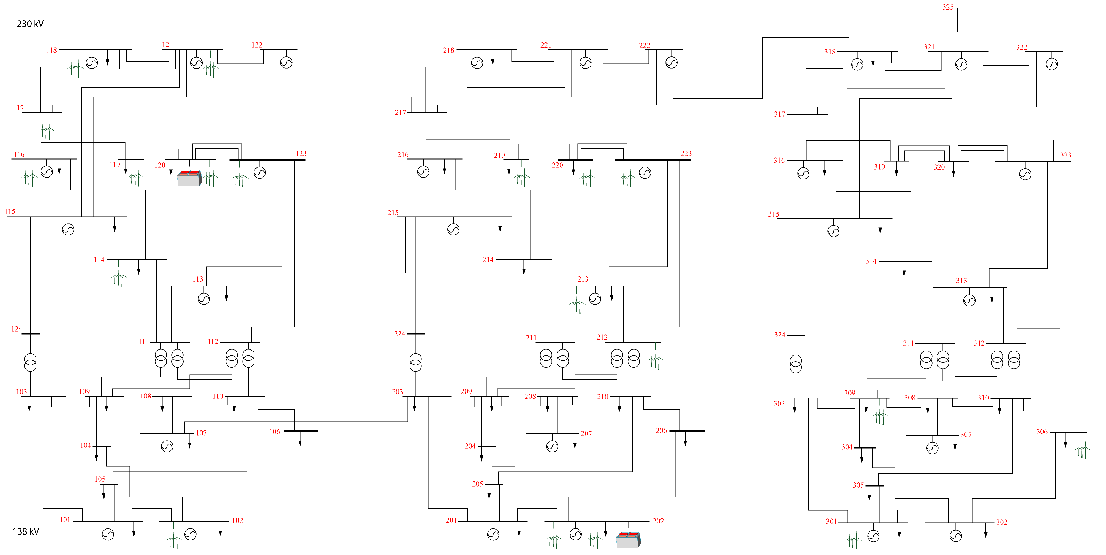
Both of the proposed models are tested on a modernized IEEE RTS-96 system, as shown in Figure 1 [19], with wind power plants and ESS devices [23,25]. The case study network consists of three areas, where the first area contains nine wind farms (w1–w9) with overall capacity of 3900 MW; the second area contains six wind farms (w10–w16) with overall capacity of 2400 MW; and the third area contains three wind farms (w17–w19) with overall capacity of 300 MW. Although the test system is a generic IEEE network, the wind topography replicates the Electric Reliability Council Of Texas (ERCOT) system, where the power flows are directed from the west zone, with abundant wind generation, to the east zone, with large loads [26]. ESS units are connected to buses where the significant wind power is injected into the grid.
The test system contains 96 conventional generators (overall capacity 10,215 MW), 19 wind farms (overall capacity 6900 MW), two ESS units of 100 MW and 600 MWh each connected to Buses 120 and 202. Both charging and discharging efficiencies of ESS are 0.90. The initial and final ESS state of charge is 50%.
The generated wind output data are based on 10-min wind speed data applied to aggregated Vestas V90-3 MW wind turbines to obtain power outputs at locations in the western USA in the period of 2004–2006. These data are a part of the NREL’s Western Wind dataset [27]. The dataset contains 32,043 sites, which are combined in order to signify the locations of large capacity wind farms connected at buses into the transmission network. The wind speed data from the database were first converted into the wind power data using the wind turbine power curve. The data from 2004–2005 were selected as input in the model, while the data from 2006 were used in the process of calibration. Similarly to [28], the first step is to normalize the wind speed data in a way that each point is subtracted by the average of the corresponding month, and the second step is to divide it by the standard deviation of the corresponding hour of the month. The following step is to obtain stationary Gaussian distributed series by the undesirable data with the empirical distribution function. These time series are fitted to normalized data, as elaborated in [19]. Every model is updated with a step of six hours in which data are used by the 120 most recent hours of wind data in 2006, and followed by each update, each model provides a new six-hour prediction. Following a scenario reduction technique from [29], we used four representative days from this dataset.
The production of wind farms is shown in Figure 2. We compare ESS performance for the following four cases: (1) high wind generation throughout the day; (2) low wind generation; (3) high wind generation in the second half of the day and (4) high wind generation in the first half of the day. Both models are tested on these four representative days.
3.1. Vertically-Integrated Power System
First, the model is tested without any ESS in order to determine the baseline result, which is compared to the results obtained with ESS in the system. The overall system cost with and without ESS is shown in Table 1 (last three rows). The presence of ESS brings savings in the range of 0.2–1.3%. The lowest savings are achieved on Day 2, which has the lowest wind output, while the highest savings are achieved on Day 1, which has the most wind. This indicates that ESS results in the highest operating cost savings on days with the most wind energy. ESS acts in a way to reduce wind curtailment. On Day 1, ESS operation reduces wind curtailment by 8.4% (last two rows in Table 2). On Day 2, due to low wind, there is no curtailment, even without ESS. Day 3 has very similar curtailment values of wind curtailment as Day 1, although the hourly distribution is different. Day 4 has lower wind curtailment than Day 1 and Day 3, and ESS operation reduces it by 9.3%.
Overall generation throughout the day changes in the presence of ESS. On the one hand, ESS reduces wind curtailment, which decreases the amount of electricity generators need to produce. On the other hand, ESS have round trip efficiencies that are lower than 100%. On Days 1, 2 and 4, the wind curtailment is greater than the electricity lost due to ESS inefficiency, resulting in decreased overall electricity produced by conventional generators (first two rows in Table 2). On Day 2, there is no wind curtailment, which means than any ESS activity increases the overall conventional electricity generation. ESS also affects the peak production of conventional generators. In all four cases, peak generation is reduced by 200 MW, which is the output capacity of ESS in the system (first two rows in Table 1). These results show the role ESS can have in the reduction of cycling of peaking units, but also in deferring generation capacity system-wide.
Daily charging and discharging cycles of both ESS units during four representative days are presented in Figure 3. In all of the cases, both ESS are finished charging by Hour 7. On Day 1, ESS are fully discharged by Hour 11, when abundant wind output starts. High wind output supplies most of the load during the afternoon. Evening reduced load hours are used to charge the ESS to the requested 50% state of charge. Low wind output is used to fully charge ESS in the early hours of Day 2 (the maximum state of charge of ESS is 540 MWh, due to charging efficiency). Approximately 300 MWh is discharged from each ESS in 17–19 to reduce the running of peaking units for supplying the high evening load. The last hour is used for recharging ESS to the required 50% of state of charge. On Day 3, ESS are fully charged by the morning, and they discharge during the morning peak hours due to scarce wind production. Abundant wind power in the later hours is used to supply the evening peak consumption and to charge ESS. Day 4 operation of ESS is very similar to Day 2. Part of the copious wind generation in the early hours is used to charge ESS, but most of it is curtailed due to low consumption. ESS are discharge in the late afternoon and evening to reduce the impact of high-cost peaking units.
3.2. Market-Based Power System
The goal of the market-based model is to maximize the overall ESS profit. The overall ESS profit for each of the four days is shown in Table 3. ESS profit highly depends on the wind profile. Day 2, where wind generation is low throughout the day, provides very limited profit opportunities for ESS, resulting in only a 2272 € profit. Figure 4b shows a rather flat LMP profile at Buses 120 and 202. Day 1, on the other hand, has high wind generation throughout the day and results in much higher ESS profit. Figure 4a shows much higher variability of LMPs at both ESS buses. Days 3 and 4 have uneven wind generation throughout the day, which results in high differences in LMPs. Volatile LMPs enable ESS to attain a high difference in purchasing and selling prices, which results in over a 12,000 profit on Day 3 and Day 4.
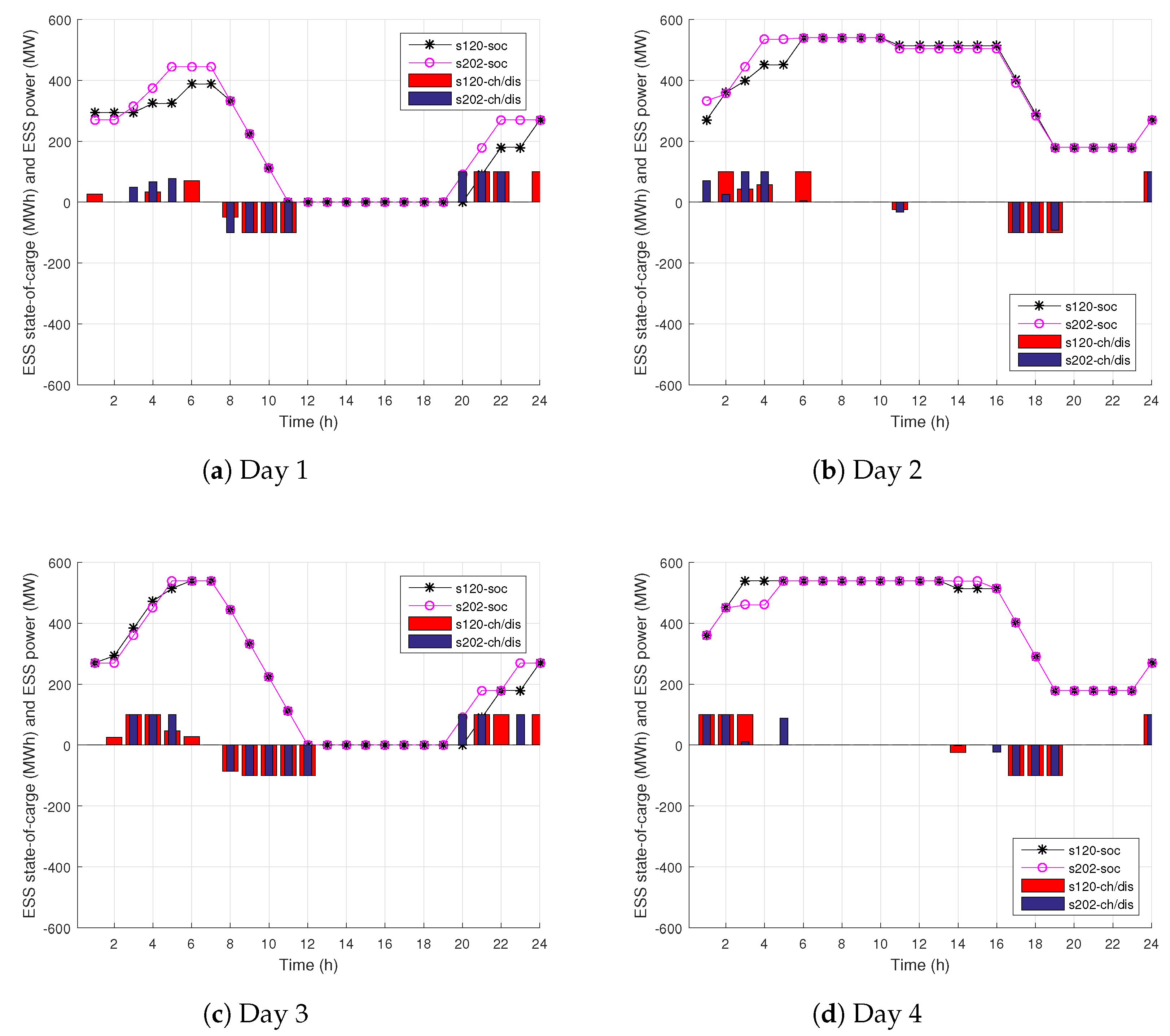
ESS operation in market-based environment is shown in Figure 5. On representative Day 1, ESS at Bus 202 is not charged in the morning due to relatively high LMPs (compare with Figure 4a). Instead, only ESS at Bus 120 is charged, due to lower LMPs. Since the LMPs are highest in Time Periods 8–11, both ESS are discharged in the late morning. LMPs at Bus 202 fall to zero at Hour 18 and stay zero until the end of the day, which is why ESS at Bus 202 is charged to the required capacity in the late evening. LMPs at Bus 120 are lowest towards the end of the day, as well, making this time of the day favorable for charging. On Day 2, both ESS fully charge in the morning. Although the morning prices are higher than on Day 1, both ESS fully charge because the afternoon LMPs are much higher, making it profitable for ESS to perform arbitrage. Days 3 and 4 are similar in the way that ESS charge in the morning and discharge during peak price hours. For Day 3, these peak price hours are 8–12, while for Day 4, they occur in the late afternoon. Note that ESS at Bus 202 performs arbitrage between Hours 2 and 3 of Day 4 due to the local price spike.
Social welfare for all four representative days in cases with and without ESS is presented in Table 4. The presence of ESS increases social welfare by up to 1%. It is interesting to compare ESS profit from Table 3 with the increase of social welfare in Table 4. The conclusion is that relatively small ESS profit results in much higher improvement of social welfare. For instance, a 9376 € ESS profit on Day 1 causes an 82,830 € increase in social welfare. This is because the social welfare is not only increased by storage offers and bids, but also because of higher utilization of wind energy.
Table 5 shows peak production, overall daily production and wind curtailment with and without ESS in the market-based power system. Like in the vertically-integrated model, peak production of conventional generating units is reduced by 200 MW, i.e., the ESS capacity. Overall generation is reduced on Days 1, 3 and 4, while on Day 2, it is increased due to low wind output (no wind curtailment even in the no ESS case). Wind curtailment is reduced on all representative days. Generally, wind curtailment is much lower in the market-based system as compared to the vertically-integrated system. This is the result of more stringent constraints in the vertically-integrated system, e.g., generator minimum generation, minimum up and down times, start-up costs. These constraints are not part of the market-based model. They are subject to self-scheduling and out-of-market corrections.
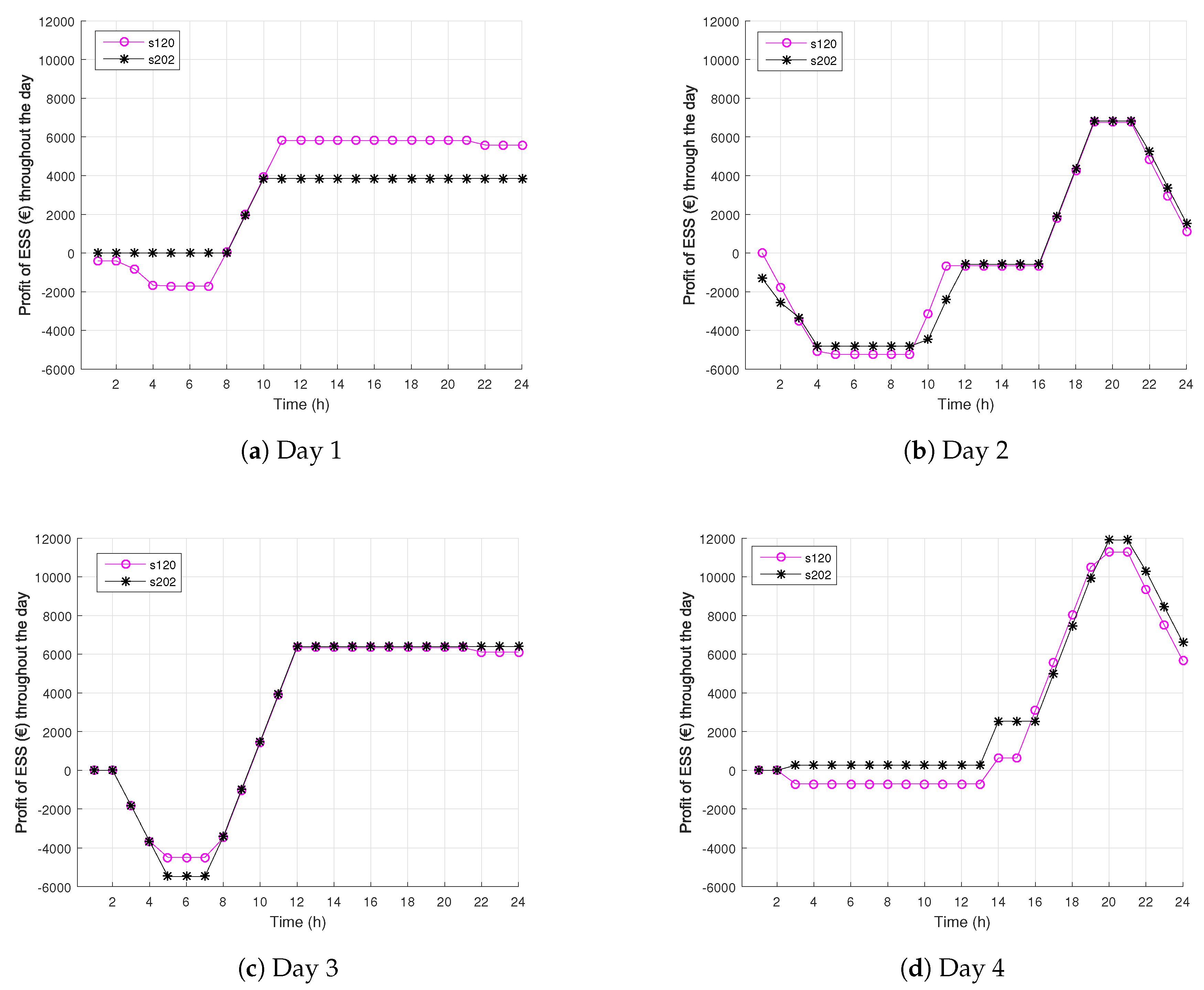
Figure 6 shows cumulative ESS profit throughout the day for each representative day. In almost all cases, ESS first purchases energy, resulting in negative profit, then sells energy, reaching its positive peak profit. The profit is then decreased in most of the cases because of the constraint imposing 50% state of charge at the end of the time horizon. During Day 1, ESS at Bus 202 does not start with negative profit (Figure 6a) because this ESS is not charged during the night (Figure 5a). During Day 4, ESS at Bus 202 is charged at zero LMP and performs arbitrage between Hours 2 and 3, which brings it to a positive profit in the early hours (Figure 6a).
4. Conclusions
The presented simulation results indicate that ESS benefits in both vertically-integrated and market-based power systems. In the vertically-integrated system, the savings achieved by two distributed ESS result in saving up to 1.3%. The savings are greater for days with high wind outputs. This result indicates that power systems with high penetration of renewable generators benefit from ESS the most. Furthermore, ESS reduces wind curtailment, which reduces the generation of conventional generators. Peak production of conventional generators is reduced, as well.
In the market-based power system, ESS collects profit based on the difference in LMPs throughout the day. Even relatively low ESS profit results in a much higher (up to 10-times) increase in social welfare. One reason for this is the ESS market offers and bids, while the other reason, much more significant, is the reduction of wind curtailment. An additional finding is that ESS offers and bids for electricity in a way that is as neutral as possible for LMPs. ESS market actions that affect LMPs disrupt its profit opportunities. Therefore, one cannot expect significant price deviations as a result of ESS operation.
Although ESS can make a profit in the energy market, these profits are insufficient to justify such investment. Therefore, multiple streams of revenue need to be stacked together to justify investment in ESS. Our future work will be focused on ESS as a reserve provider and a temporary means for the deferral of investment in transmission and generation.
Acknowledgments
This work has been supported in part by Croatian Science Foundation and Croatian Transmission Operator System (TSO) under the project Smart Integration of RENewables (I-2583-2015).
Author Contributions
Hrvoje Pandžić conceived and designed the experiments; Zora Luburić performed the experiments and performed literature review; Tomislav Plavšić analyzed the data and designed the experiments.
Conflicts of Interest
The authors declare no conflict of interest.
Abbreviations
The following abbreviations are used in this manuscript:
| ERCOT | Electric Reliability Council Of Texas |
| ESS | Energy storage system |
| GAMS | General algebraic modeling system |
| KKT | Karush–Kuhn–Tucker |
| LMP | Local marginal price |
| LOLP | Loss of load probability |
| MILP | Mixed integer programming problem |
| RES | Renewable energy sources |
| TSO | Transmission system operator |
| Nomenclature | |
| B | energy system units, indexed by b |
| C | segments of generators cost curves, indexed by c |
| I | thermal generator units, indexed by i |
| L | lines, indexed by l |
| N | buses, indexed by n |
| T | time periods, indexed by t |
| W | wind farms, indexed by w |
| Parameters | |
| maximum charging capacity of ESS b (MWh) | |
| maximum demand at bus n during time period t (MW) | |
| maximum discharging capacity of ESS b (MWh) | |
| fixed production cost of generator i (€) | |
| maximum capacity of segment c of generator i cost curve (MW) | |
| minimum capacity of generator i cost curve (MW) | |
| ON-OFF status of generator i at time t (1/0) | |
| minimum down time of generator i (h) | |
| minimum up time of generator i (h) | |
| maximum power production of wind farm w during time period t (MW) | |
| slope of the segment c of the cost curve of generator i (€/MW) | |
| maximum power flow through line l (MW) | |
| ramp-down limit of generator i (MW/h) | |
| ramp-up limit of generator i (MW/h) | |
| maximum capacity of ESS b (MWh) | |
| minimum capacity of ESS b (MWh) | |
| susceptance of line connecting buses n-m (S) | |
| charging efficiency of ESS b (-) | |
| discharging efficiency of ESS b (-) | |
| length of time that generator i must be OFF at the start of the planning horizon (h) | |
| length of time that generator i must be ON at the start of the planning horizon (h) | |
| Variables | |
| demand at bus n (MW) in dispatch hour t | |
| generator production i by block c (MW) in dispatch hour t | |
| power production of wind farm w (MW) in dispatch hour t | |
| power flow through line l (MW) in dispatch hour t | |
| state of charge of ESS b (MWh) in dispatch hour t | |
| start-up cost of generator i at time t (€) | |
| voltage angle at bus n (rad) in dispatch hour t | |
| charging power purchased by ESS b (MW) in dispatch hour t | |
| discharging power sold by ESS b (MW) in dispatch hour t | |
| Binary Variables | |
| enforces ESS b to bid; 1 when charging in dispatch hour t | |
| enforces ESS b to offer; 1 when discharging in dispatch hour t | |
| 1 if generator i is producing at time t, 0 otherwise | |
| 1 if generator i is started at time t, 0 otherwise | |
| 1 if generator i is shutdown at time t, 0 otherwise |
References
- US DOE Energy Information Administration/Electric Power Monthly. Available online: http://www.eia.gov/electricity/monthly/ (accessed on 25 April 2017).
- EWEA (The European Wind Energy Association). Wind in Power 2015 European Statistics; EWEA: Leuven, Belgium, 2016. [Google Scholar]
- Fabbri, A.; San Roman, T.G.; Abbad, J.R.; Quezada, V.H.M. Assessment of the Cost Associated with Wind Generation Prediction Errors in a Liberalized Electricity Market. IEEE Trans. Power Syst. 2005, 20, 1440–1446. [Google Scholar] [CrossRef]
- Ortega-Vazquez, M.; Kirschen, D.S. Assessing the Impact of Wind Power Generation on Operating Costs. IEEE Trans. Smart Grid 2010, 1, 295–301. [Google Scholar] [CrossRef]
- Baringo, L.; Conejo, A.J. Strategic Offering for a Wind Power Producer. IEEE Trans. Power Syst. 2013, 28, 4645–4654. [Google Scholar] [CrossRef]
- Zugno, M.; Morales, J.M.; Pinson, P.; Madsen, H. Pool Strategy of a Price-Maker Wind Power Producer. IEEE Trans. Power Syst. 2013, 28, 3440–3450. [Google Scholar] [CrossRef]
- Delikaraoglou, S.; Papakonstantinou, A.; Ordoudis, C.; Pinson, P. Price-Maker Wind Power Producer Participating in a Joint Day-Ahead and Real-Time Market. In Proceedings of the 12th International Conference on the European Energy Market (EEM), Lisbon, Portugal, 19–22 May 2015; pp. 1–5. [Google Scholar]
- Aigner, T.; Jaehnert, S.; Doorman, G.L.; Gjengedal, T. The Effect of Large-Scale Wind Power on System Balancing in Northern Europe. IEEE Trans. Sustain. Energy 2012, 3, 751–759. [Google Scholar] [CrossRef]
- Taczi, I.; Szorenyi, G. Pumped Storage Hydroelectric Power Plants: Issues and Applications; Energy Regulators Regional Association (ERRA): Budapest, Hungary, 2016. [Google Scholar]
- Office of Electricity Delivery and Energy Reliability. Available online: http://energy.gov/ (accessed on 8 May 2012).
- Pozo, D.; Contreras, J.; Sauma, E.E. Unit Commitment With Ideal and Generic Energy Storage Units. IEEE Trans. Power Syst. 2014, 29, 2974–2984. [Google Scholar] [CrossRef]
- Yan, N.; Xing, Z.X.; Li, W.; Zhang, B. Economic Dispatch Application of Power System with Energy Storage Systems. IEEE Trans. Appl. Superconduct. 2016, 26, 0610205. [Google Scholar] [CrossRef]
- Li, N.; Uçkun, C.; Constantinescu, E.M.; Birge, J.R.; Hedman, K.W.; Botterud, A. Flexible Operation of Batteries in Power System Sceduling with Renewable Energy. IEEE Trans. Power Sustain. Energy 2016, 7, 685–696. [Google Scholar] [CrossRef]
- Kyriakopoulos, G.L.; Arabatzis, G. Electrical energy storage systems in electricity generation: Energy policies, innovative technologies, and regulatory regimes. Renew. Sustain. Energy Rev. 2016, 56, 1044–1067. [Google Scholar] [CrossRef]
- Kyriakopoulos, G.L.; Arabatzis, G.; Chalikias, M. Renewables exploitation for energy production and biomass use for electricity generation. A multi-parametric literature-based review. AIMS Energy 2016, 4, 762–803. [Google Scholar] [CrossRef]
- Sioshansi, R.; Madaeni, S.H.; Denholm, P. A Dynamic Programming Approach to Estimate the Capacity Value of Energy Storage. IEEE Trans. Power Syst. 2014, 29, 395–403. [Google Scholar] [CrossRef]
- Wogrin, S.; Gayme, D.F. Optimizing Storage Siting, Sizing, and Technology Portofolios in Transmission- Constrained Networks. IEEE Trans. Power Syst. 2015, 30, 3304–3313. [Google Scholar] [CrossRef]
- Meneses de Quevedo, P.; Contreras, J. Optimal Placement of Energy Storage and Wind Power under Uncertainty. Energies 2016, 9, 528. [Google Scholar] [CrossRef]
- Pandžić, H.; Wang, Y.; Qiu, T.; Dvorkin, Y.; Kirschen, D.S. Near-Optimal Method for Siting and Sizing of Distributed Storage in a Transmission Network. IEEE Trans. Power Syst. 2015, 30, 2288–2300. [Google Scholar] [CrossRef]
- Dvorkin, Y.; Fernandez-Blanco, R.; Kirschen, D.S.; Pandžić, H.; Watson, J.-P.; Silva-Monroy, C.A. Ensuring Profitability of Energy Storage. IEEE Trans. Power Syst. 2016, 32, 611–623. [Google Scholar] [CrossRef]
- Hu, Z.; Zhang, S.; Zhang, F.; Lu, H. SCUC with Battery Energy Storage System for Peak-Load Shaving and Reserve Support. In Proceedings of the 2013 IEEE Power and Energy Society General Meeting (PES), Vancouver, BC, Canada, 21–25 July 2013; pp. 1–5. [Google Scholar]
- Sioshansi, R.; Denholm, P.; Jenkin, T. Market and Policy Barriers to Deployment of Energy Storage; Economics of Energy and Environmental Policy: Cleveland, OH, USA, 2012; p. 1. [Google Scholar]
- Pandžić, H.; Kuzle, I. Energy Storage Operation in the Day-Ahead Electricity Market. In Proceedings of the IEEE Conference on the European Energy Market, Lisbon, Portugal, 19–22 May 2015; pp. 1–6. [Google Scholar]
- Miranda, I.; Silva, N.; Bernardo, A.M. Assessment of the potential of Battery Energy Storage Systems in current European markets designs. In Proceedings of the 12th International Conference on the European Energy Market (EEM), Lisbon, Portugal, 19–22 May 2015; pp. 1–5. [Google Scholar]
- The IEEE Reliability Test System. A report prepared by the Reliability Task Force of the Application of Probability Method Subcommittee. IEEE Trans. Power Syst. 1999, 14, 1010–1020. [Google Scholar]
- Baldick, R. Wind and Energy Markets: A Case Study of Texas. IEEE Syst. J. 2012, 6, 27–34. [Google Scholar] [CrossRef]
- Potter, C.W.; Lew, D.; McCaa, J.; Cheng, S.; Eichelberger, S.; Grimit, E. Creating the Dataset For the Western Wind and Solar Integration Study (USA). Wind Eng. 2008, 32, 325–338. [Google Scholar] [CrossRef]
- Papavasiliou, A.; Oren, S.S. Multiarea Stochastic Unit Commitment For High Wind Penetration in a Transmission Constrained Network. Oper. Res. 2013, 61, 78–592. [Google Scholar] [CrossRef]
- Growe-Kuska, N.; Heitsch, H.; Romisc, W. Scenario Reduction and Scenario Tree Construction for Power Management Problems. In Proceedings of the IEEE Bologna Power Technology Conference, Bologna, Italy, 23–26 June 2003. [Google Scholar]
Figure 1.
IEEE RTS network.

Figure 2.
Wind production by 19 wind farms.
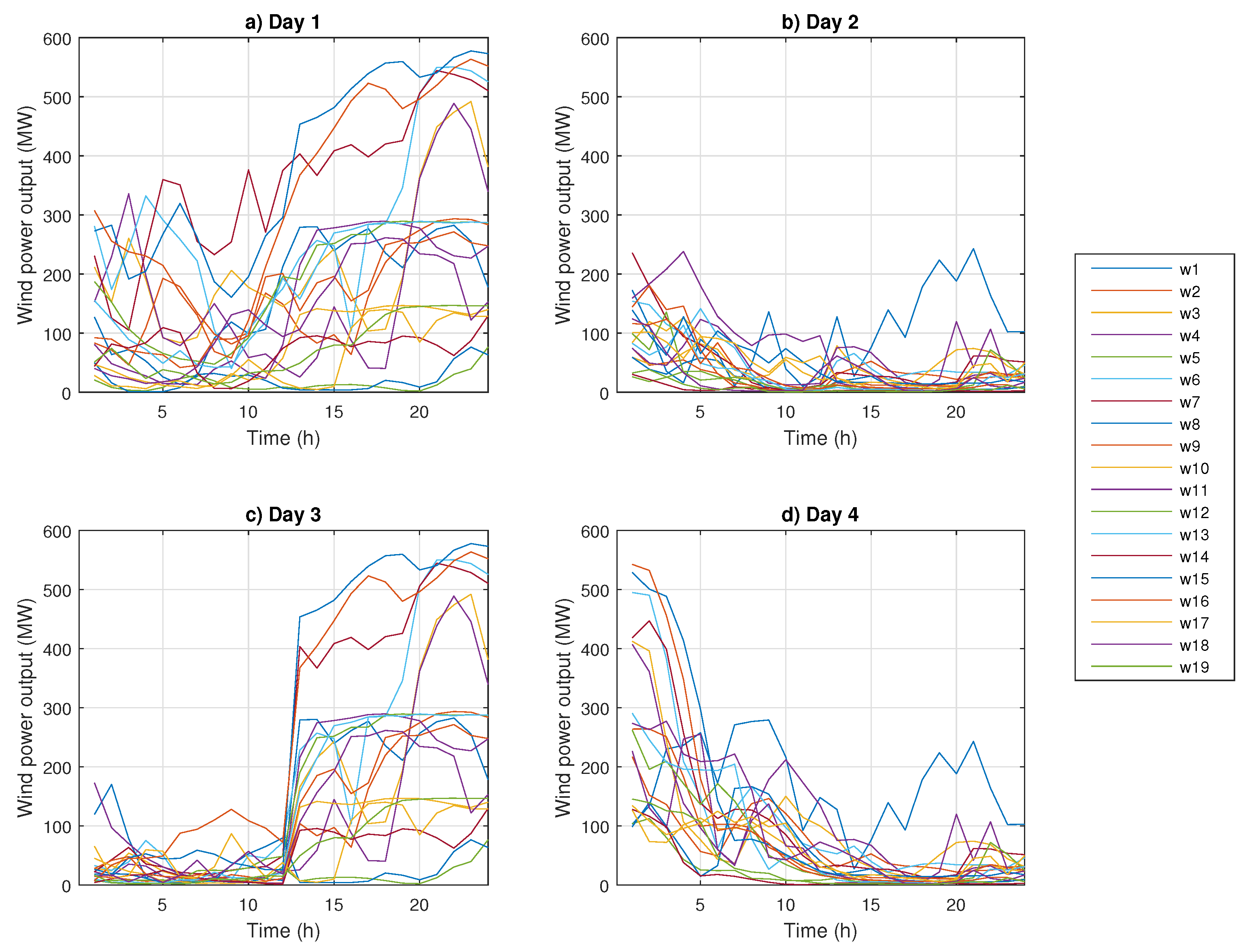
Figure 3.
ESS operation in the vertically-integrated power system.

Figure 4.
Local marginal prices at Buses 120 and 202.
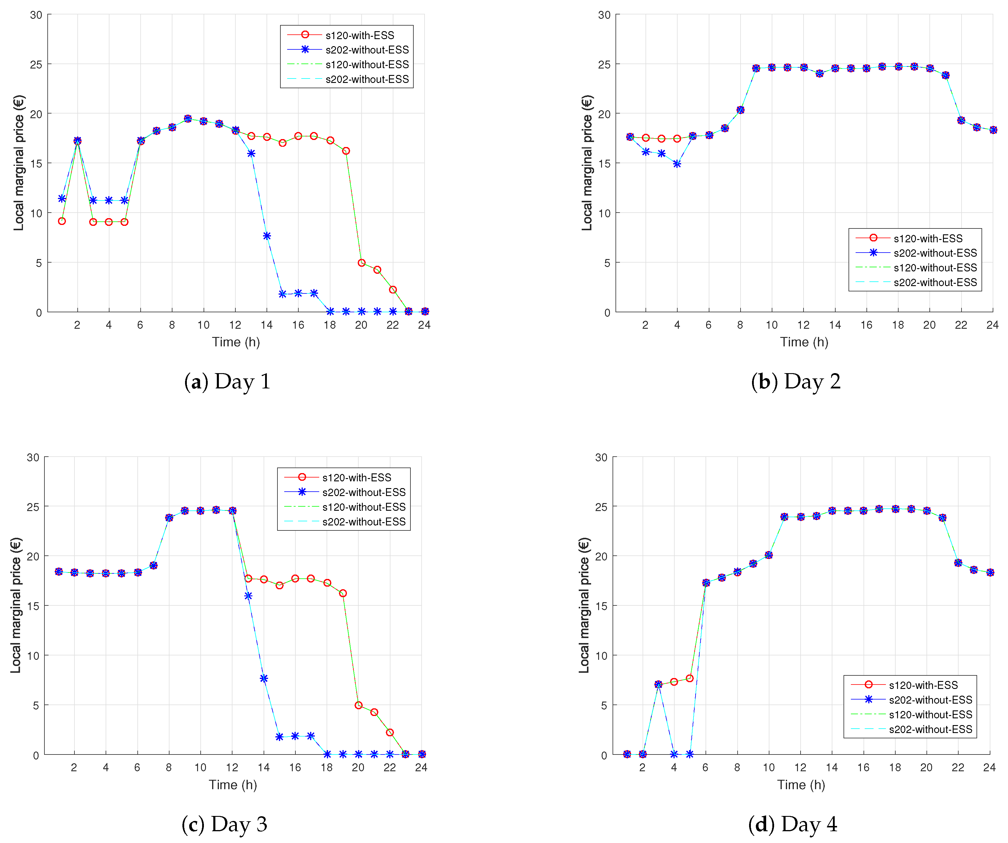
Figure 5.
ESS operation in the market-based power system.
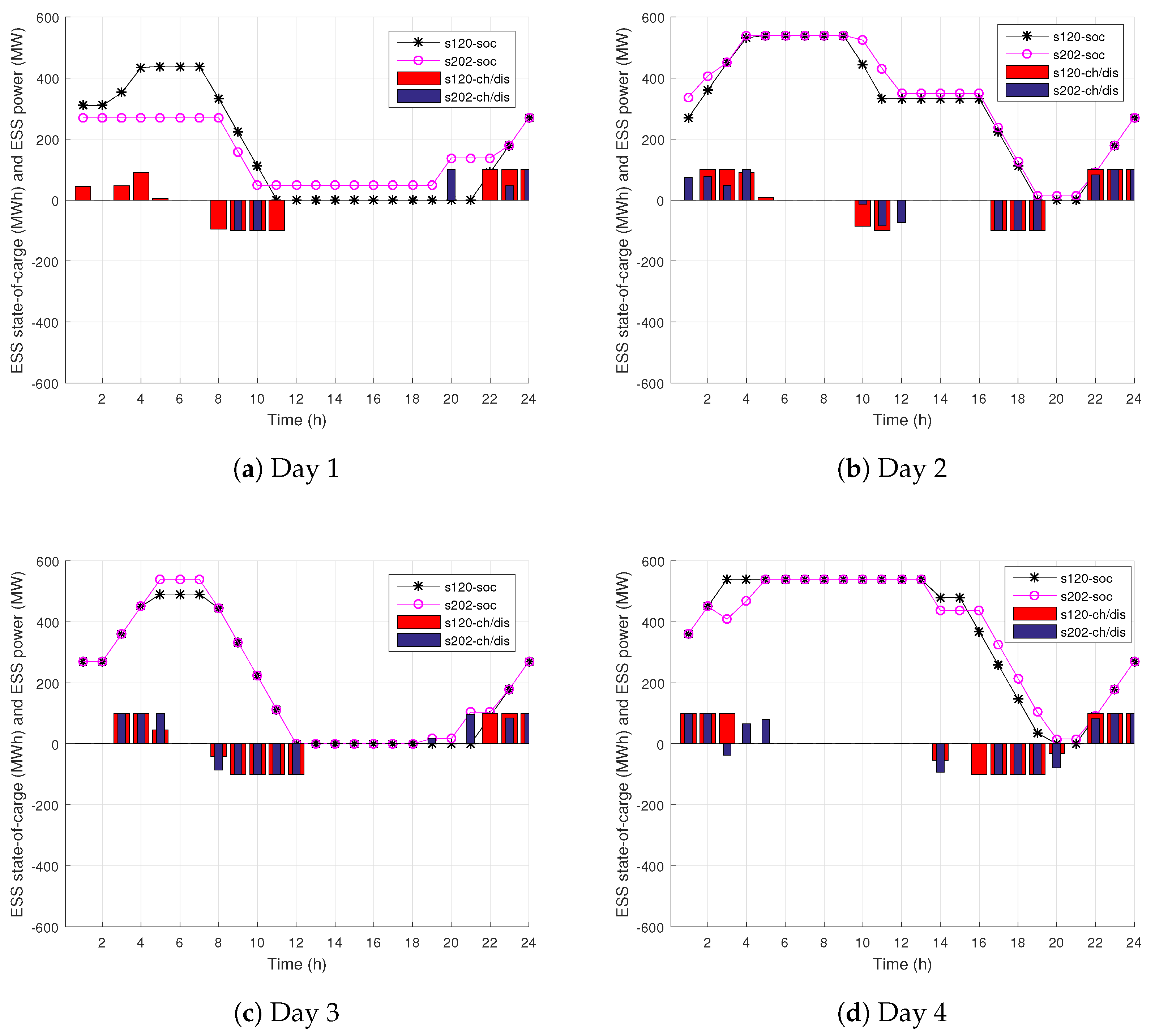
Figure 6.
ESS profit throughout the day.


Table 1.
Peak production and overall generation cost.
| Day 1 | Day 2 | Day 3 | Day 4 | |
|---|---|---|---|---|
| Peak production of conventional generators with ESS (MW) | 5436 | 6972 | 6598 | 6972 |
| Peak production of conventional generators without ESS (MW) | 5636 | 7172 | 6798 | 7172 |
| Overall generation cost with ESS (€) | 1,203,739 | 2,345,928 | 1,582,782 | 2,095,339 |
| Overall generation cost without ESS (€) | 1,219,185 | 2,351,232 | 1,599,738 | 2,111,110 |
| Overall generation cost savings | 1.3% | 0.2% | 1.1% | 0.8% |
Table 2.
Overall daily production and wind curtailment with and without ESS in the vertically-integrated power system.
Table 2.
Overall daily production and wind curtailment with and without ESS in the vertically-integrated power system.
| Day 1 | Day 2 | Day 3 | Day 4 | |
|---|---|---|---|---|
| Daily production of conventional generators with ESS (MWh) | 79,436 | 132,381 | 97,189 | 119,067 |
| Daily production of conventional generators without ESS (MWh) | 79,861 | 132,229 | 97,561 | 119,515 |
| Wind curtailment with ESS (MWh) | 6568 | 0 | 6568 | 5828 |
| Wind curtailment without ESS (MWh) | 7168 | 0 | 7168 | 6428 |
Table 3.
ESS profit in the market-based power system.
| Day 1 (€) | Day 2 (€) | Day 3 (€) | Day 4 (€) |
|---|---|---|---|
| 9376 | 2272 | 12,377 | 12,018 |
Table 4.
Social welfare in the market-based power system.
| Day 1 | Day 2 | Day 3 | Day 4 | |
|---|---|---|---|---|
| Without ESS (€) | 14,211,540 | 13,176,030 | 13,871,820 | 13,439,810 |
| With ESS (€) | 14,294,370 | 13,296,560 | 13,998,800 | 13,574,660 |
| Improvement | 0.6% | 0.9% | 0.9% | 1.0% |
Table 5.
Peak production, overall daily production and wind curtailment with and without ESS in the market-based power system.
Table 5.
Peak production, overall daily production and wind curtailment with and without ESS in the market-based power system.
| Day 1 | Day 2 | Day 3 | Day 4 | |
|---|---|---|---|---|
| Peak production of conventional generators with ESS (MW) | 5436 | 6972 | 6598 | 6972 |
| Peak production of conventional generators without ESS (MW) | 5636 | 7172 | 6798 | 7172 |
| Production of conventional generators with ESS (MWh) | 74,367 | 132,454 | 92,093 | 113,745 |
| Production of conventional generators without ESS (MWh) | 74,757 | 132,229 | 92,457 | 114,033 |
| Wind curtailment with ESS (MWh) | 1534 | 0 | 1483 | 425 |
| Wind curtailment without ESS (MWh) | 2064 | 0 | 2064 | 946 |
© 2017 by the authors. Licensee MDPI, Basel, Switzerland. This article is an open access article distributed under the terms and conditions of the Creative Commons Attribution (CC BY) license (http://creativecommons.org/licenses/by/4.0/).
Share and Cite
MDPI and ACS Style
Luburić, Z.; Pandžić, H.; Plavšić, T. Assessment of Energy Storage Operation in Vertically Integrated Utility and Electricity Market . Energies 2017, 10, 683. https://doi.org/10.3390/en10050683
AMA Style
Luburić Z, Pandžić H, Plavšić T. Assessment of Energy Storage Operation in Vertically Integrated Utility and Electricity Market . Energies. 2017; 10(5):683. https://doi.org/10.3390/en10050683
Chicago/Turabian StyleLuburić, Zora, Hrvoje Pandžić, and Tomislav Plavšić. 2017. "Assessment of Energy Storage Operation in Vertically Integrated Utility and Electricity Market " Energies 10, no. 5: 683. https://doi.org/10.3390/en10050683
Note that from the first issue of 2016, this journal uses article numbers instead of page numbers. See further details here.