Reducing Fuel Consumption in Hydraulic Excavators—A Comprehensive Analysis

Institute for Fluid Power Drives and Controls (IFAS), RWTH Aachen University, 52062 Aachen, Germany
*
Author to whom correspondence should be addressed.
Energies 2017, 10(5), 687; https://doi.org/10.3390/en10050687
Submission received: 29 March 2017
/
Revised: 8 May 2017
/
Accepted: 9 May 2017
/
Published: 12 May 2017
(This article belongs to the Special Issue Energy Efficiency and Controllability of Fluid Power Systems)
Abstract
:Mobile machines, especially excavators, still consume considerable amounts of fuel during their operating lifetimes. This is not only undesirable in economic terms but also adversely affects our environment. The following paper discusses methods to lower fuel consumption by conducting a comprehensive analysis of the components comprising a hydraulic excavator and the cycles these machines perform. One of the main aims is to emphasise that a design centred on the standard definitions of efficiency, especially hydraulic efficiency, can be rather misleading. A new approach using a novel fuel consumption model, based on the Willans approximation, coupled with the concepts of fixed and variable fuel consumption is introduced and validated using real test data obtained from an 18 t excavator. The new methodology can be used to help uncover simpler methods to improve today’s machines.
1. Introduction
Hydraulic excavators are responsible for approximately 60% of the CO2 emissions produced by construction machinery [1]. This is in part due to the sheer number of machines in use and also to their extremely low efficiencies of around 10% [2]. Despite their immense impact on our environment many aspects regarding the exact reasons for their high fuel consumption remain misunderstood. The hydraulic systems used to power these machines are often unjustly blamed for the majority of the losses. As a result, much research has gone into the development of more efficient hydraulic architectures capable of lowering so-called throttling losses and enabling energy recovery. Much less attention has been paid to the machine as a whole.
The following work aims to clarify many issues and myths surrounding hydraulic excavators by guiding the reader through a comprehensive analysis of the whole machine. The losses occurring in components and subsystems are explained and a detailed discussion of measurement data, obtained from field tests with an 18 t machine, is presented. These thoughts ultimately lead to the introduction of a novel fuel consumption model, capable of describing and predicting the fuel consumption of a machine for all duty cycles. Instead of using the widespread definitions of machine and hydraulic efficiency, the concepts of fixed and variable fuel consumption are introduced. An important aspect of the research is the validation of the methodology using real measurement data.
The authors hope to provide a tool that can be used by engineers, during the initial design phase, to easily evaluate the fuel saving potential of different architectures before running complex system simulations. As an example, solutions involving independent metering, displacement control and hybridization are discussed. Along with a brief summary, the paper concludes with an outlook concerning future work.
2. Review of Components and Subsystems
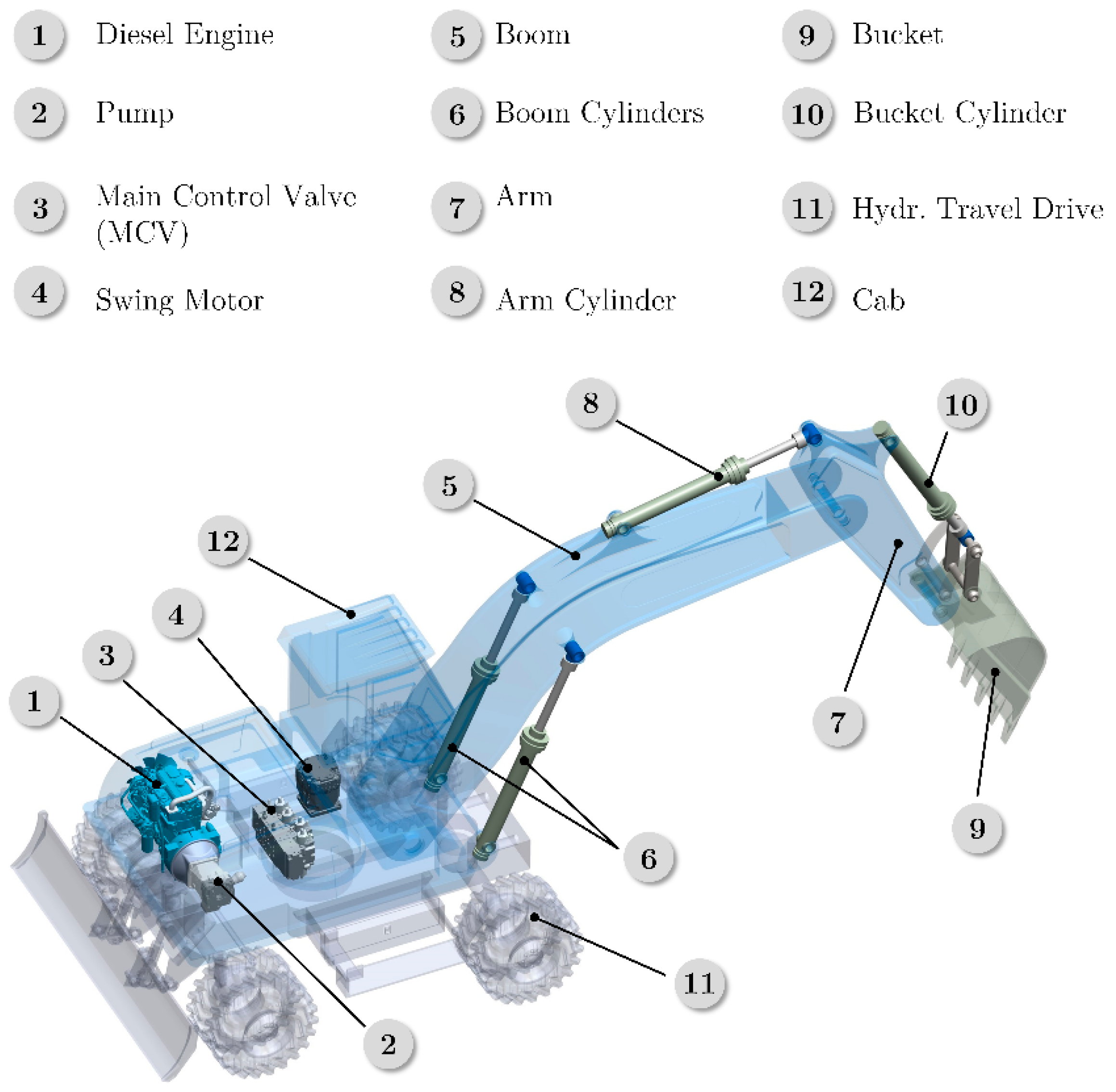
Figure 1 illustrates the typical layout and individual components of a state of the art machine. One or several hydraulic pumps, powered by a diesel engine, provide pressurised flow to the system. Using joysticks in the cab, the operator controls a series of directional valves located in a manifold block, often referred to as the main control valve (MCV). These allow an intuitive and precise distribution of the incoming pump flow to the individual actuators of the implement structure (boom, arm, bucket, swing) and travel drive. A wheeled machine with a bucket attached as a tool is shown in the figure, but various other arrangements with tracks and other specialised attachments, such as hydraulic hammers and scissors, can be found.
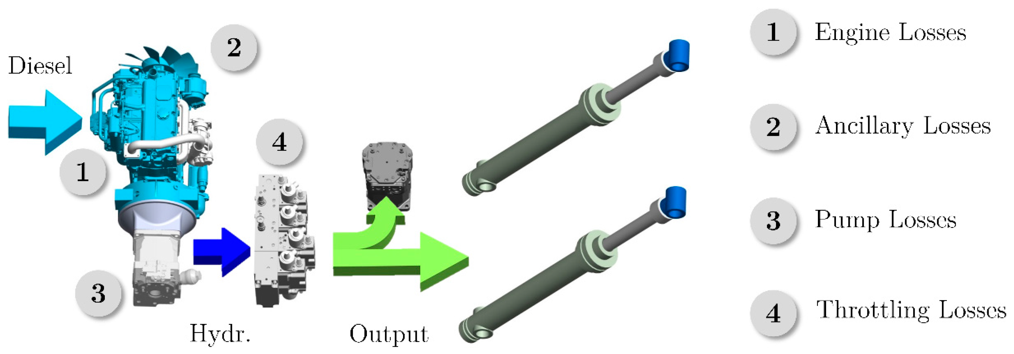
The flow of power through the machine and location of the individual losses are depicted in Figure 2. The conversion of energy from one form into another, as performed by the engine and pump(s), is the first source of losses. The second, referred to as throttling losses, is a direct consequence of using valves to distribute hydraulic power. Finally, the ancillary drives required for vital functions, such as steering, braking and cooling, are considered losses as they consume energy and do not directly contribute to the execution of the required task.
The exact reasons for these losses and their importance can be derived by analysing the individual machine subsystems and their interactions with one another in more detail. Let us begin by discussing the engine.
2.1. Engine
In theory, an engine can reach an efficiency of up to 100%, as the chemical input and mechanical output energies are both ordered and of the same quality, i.e., have the same exergy [3,4]. Unfortunately, converting chemical energy directly into mechanical work proves difficult and the fuel must first be ignited in an unconstrained chemical reaction generating heat and losses. As a result, engines specifically designed and optimised to work at a specific operating point can push their peak efficiency into a region of 45–50% but the typical units found in construction machinery display maximum efficiencies of just over 40% [5]. This value changes considerably depending on the load, i.e., torque, and speed at which the engine operates. An exemplary internal combustion engine (ICE) efficiency map is shown in Figure 3a.
The map is bounded by the full load line , which corresponds to the maximum torque or power the ICE can generate at each rotation speed. If the ICE is operated along this line, no additional acceleration torque is available. Load torques above this value lead to a deceleration of the output shaft. Only above the minimum rotation speed of about 800 rpm can an engine generate enough mechanical power to overcome its internal losses. Typical units provide a substantial acceleration torque at rotation speeds larger than 1000 rpm [6]. As the speed increases and more power can be generated, the efficiency starts improving. However, higher speeds also lead to increased friction losses and allow less time for the reactants to mix during the combustion process. As a result, efficiency first increases and then begins decreasing with speed. The so-called sweet spot in the contour plot is therefore usually located in the lower to mid-speed range just below the full load line.
Efficiency maps are characterised by curves of constant power, hyperbolas. Not every power curve passes through the optimal operating region, indicating that the unit can only function efficiently within a certain power range. When selecting an engine for a specific application, in this case an excavator, the designer must take into account the peak power demand of the hydraulic system driven by the engine. In most engines, the rotation speed , at which maximum power is available, is considerably higher than the speed at which maximum efficiency is attained. In order to deliver peak power and thereby avoid having to change the engine speed during a working cycle, standard excavators are frequently operated at a fixed engine speed, namely . During such a cycle, the load pressure and pump displacement will vary constantly, leading to fluctuations in the load torque shown in grey in Figure 3a. This results in frequent part loading and therefore inefficient engine utilisation [7].
Thinking in terms of absolute efficiency can be misleading, as fuel consumption is, in fact, the quantity that really matters. The Willans approximation, illustrated in Figure 3b, is another method of plotting engine performance and reveals some interesting aspects that are not so evident from the contour plotted efficiency map [8]. The fuel consumption of an engine at a constant speed increases approximately linearly with its output power. For most diesel engines, this proportionality factor takes on a value of about 0.22 L/kWh [9]. In other words, each additional kW of output power results in the same increase in the fuel consumption rate, regardless of the current operating point. What this actually means is that the engine’s differential efficiency is actually a constant with a value of 42%. The Willans lines also show that an engine delivering no power still consumes fuel due to its parasitic losses. This is referred to as the idle fuel consumption and largely depends on the engine size , the number of pistons/cylinders and rotation speed . In general, larger engines and higher rotation speeds lead to higher parasitic losses and therefore an increase in idle fuel consumption.
According to Rohde-Brandenburger, in the case of a turbocharged diesel engine, the Willans approximation can be expressed as follows [8]:
with
This is in fact the reason why cars with engine start–stop systems reduce fuel consumption. Similarly, this explains the real advantage of the concepts referred to as engine downsizing and downspeeding. It is not due to the widely cited claim that the thermodynamic efficiency of the engine improves when operating at higher loads and smaller displacements, but rather that the idle fuel consumption of a downsized or downsped engine is lower [9,10]. This concept reveals invaluable information regarding how much the fuel consumption of a vehicle can be improved without making changes to the engine. For example, in the case of an average passenger vehicle with a four cylinder engine, the idle fuel consumption is responsible for up to 50% of the total fuel consumption in the new European driving cycle (NEDC). This would mean that the maximum fuel reduction achievable, by designing a new vehicle with theoretically zero mass and zero wind resistance but without any changes to the engine and gearbox, is only 50% [9]. This highlights the importance of using smaller engines operating at lower speeds.
These observations have important consequences for the energy management strategies in hybrid vehicles. When an engine is already running, the decision to charge the battery or accumulator using the engine can be made without regarding the current operating point because the differential efficiency is constant [11]. Only when the engine is off does the decision to charge lead to additional losses due to idling.
Reducing engine losses has not been one of the main concerns of excavator manufacturers in recent years. In the late 20th century, studies proved that the particulate matter (PM), carbon monoxide (CO) and nitrous oxides (NOX) formed during the combustion of diesel fuel, are all detrimental to human health [12,13,14]. In an attempt to improve the air quality in cities and towns, governments introduced a set of stringent diesel emission standards in the 1990s. The initial TIER 1–3 standards (in Europe Stage I–III), phased in between 1998 and 2008, were met using advanced engine designs and basically no or very simple exhaust gas after-treatment methods. With the introduction of the TIER 4 interim and final (European Stage IIIB and IV) standards, which were phased in from 2008 to 2015, manufacturers first agreed to decrease PM and then NOX emissions by a further 90%. Meeting these standards was considerably more difficult.
Today’s excavators and other off-highway machines use expensive after-treatment systems with diesel oxidation catalysts (DOC) and diesel particulate filters (DPF). This has led to increased costs and a further reduction in the available installation space around the engine. As explained by Filla, the way in which emissions tests are currently conducted has also given OEMs (Original Equipment Manufacturers) little or no incentive to introduce efficient downspeed engines with hybrid technologies [15]. The official non-road transient cycle (NRTC), used to evaluate engine emissions, uses a predetermined set of engine speeds and torques, which may not even match the actual engine operation in a machine. As a result, a machine with an advanced engine management system would be no different to a standard unit in regard to the current engine emissions regulations.
All the aspects mentioned above relate to quasi-static engine performance. As shown in Figure 4 the effect of dynamic engine loading should not and cannot be neglected. In any typical excavator duty cycle, the engine load fluctuates rapidly and the engine must be able to respond quickly to these load changes to avoid stalling or excessive drops in rotation speed [16].
Depending on the extent of these transients, fuel consumption can fluctuate considerably from the quasi-static descriptions in Figure 3. Research has, in fact, shown that up to 50% of emissions are caused by transient loads [17,18]. As a result, newer TIER 4 engines do not have the same response that the older TIER 3 engines had. This is especially evident at lower engine speeds and is an important issue that will affect the design of newer mobile hydraulic systems.
The mechanical power generated by the engine, must now be distributed to the individual hydraulic actuators. This takes us to the machine’s hydraulic system.
2.2. Hydraulic System
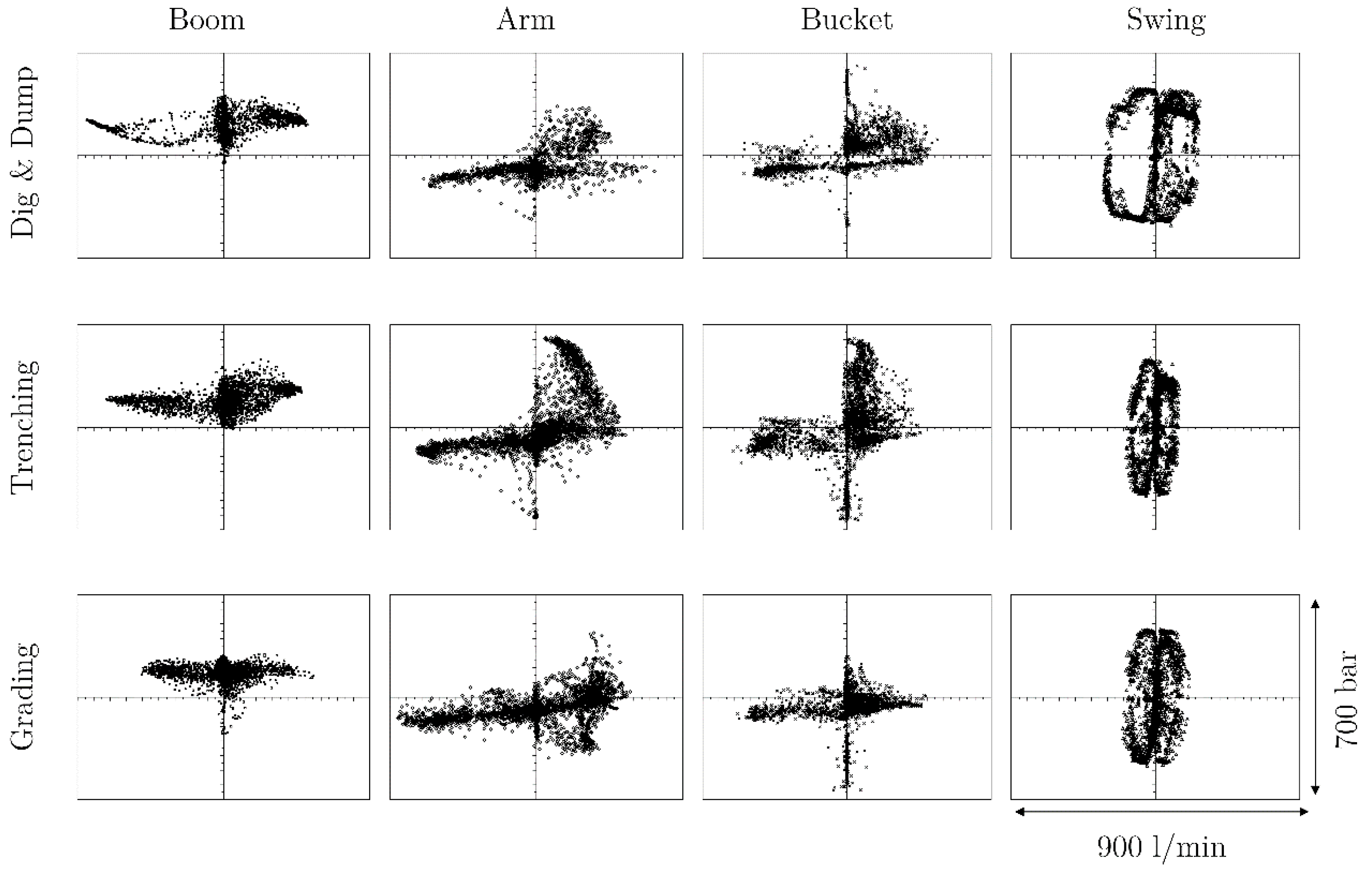
The way in which the hydraulic actuators interact with the external environmental load is particularly complex. Not only are the force and velocity demands of each actuator completely different, they also vary independently of each other depending on the operator’s commands. Some actuators may require high force and low velocity (high pressure, low flow) while others require low force and high velocity (low pressure, high flow). Figure 5 illustrates the load situation for the actuators making up the implement structure. The x-axis shows the flow required by each actuator () and can be interpreted as the operator’s input to the system. The y-axis shows the force or load pressure () experienced by the actuator and is a direct consequence of the surroundings, cf. Equations (3)–(5).
In the case of the linear actuators, the force acting on them is due to both the weight of the attached structure and the external forces present during digging and other operations. Inertial forces caused during acceleration play a less important role. Depending on the movements, each actuator experiences either a resistive force opposing its motion (Quadrants I and III) or an assistive force aiding its motion (Quadrants II and IV). Consequently, in quadrants I and III, the actuator must be actively supplied with power, while, in quadrants II and IV, the actuators can actually supply power to the system.
Due to the kinematic arrangement and large weight of the implement structure, the boom cylinders almost exclusively operate in load quadrants I and II. In contrast, the magnitude and direction of the load acting on the arm and bucket cylinders varies a great deal, causing operation in all four quadrants. The hydraulic motor driving the swing experiences four quadrant operation, but in contrast to the linear actuators the inertial forces dominate here, meaning that the load pressure is mainly due to the acceleration of the superstructure and not caused by external forces.
Each point in the plane represents a state of quasi-stationary equilibrium, in which the pump flow rate is proportional to the operator’s joystick displacement, system pressure is determined by the load, and the engine torque and pump torque are equal. As the actuator operating points move through the different load quadrants, the system’s power demand changes. To maintain a stable engine speed, every change in demand must be closely followed by a change in supply. This can be tricky for two reasons.
Firstly, the engines in most machines cannot even deliver the same amount of power as can be demanded by the pump. This may sound strange, but has to do with dimensioning. The pump size is selected to meet the maximum speed/flow rate requirements of all the actuators (implements + travel drive) when operating at the rated engine speed. System pressure is a function of the load and can reach values up to , but is typically around 200 bar. The pump’s corner power is, therefore, considerably greater than the power required during standard operation. Installing an engine with the same corner power capabilities as the pump in order to cover these infrequent cases would be expensive and require more space. As a result, it is quite common to find machines, in which the corner power of the pump is two or three times greater than the maximum engine power. Full actuator speed can only be maintained for average system pressures around 180 bar, thereafter a power limiting controller swivels the pump back preventing the engine from stalling.
Secondly, as the operator adjusts his joystick commands and the load changes, an actuator’s state can move through the load plane rather rapidly. Unfortunately, most engines cannot react so quickly to such rapid load changes and are prone to stalling. The pump controller and valves must assume this role, and ideally work in sync with the EECU, to ensure the dynamic power demand and supply are well matched. Achieving a well-tuned engine-pump interface is one of the major challenges in today’s mobile hydraulic systems [19].
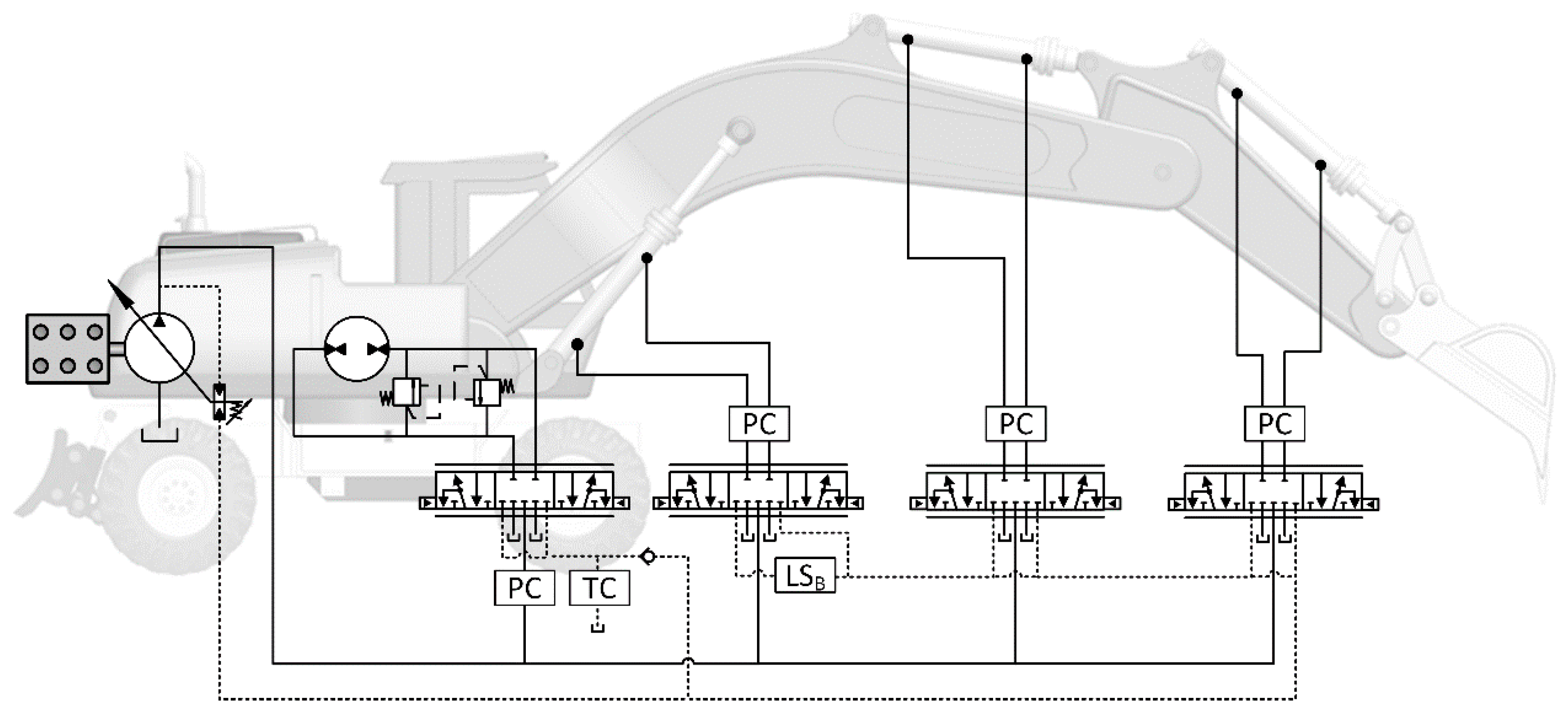
In contrast to most other mobile machines, excavators are capable of rotating their superstructure relative to the undercarriage by using the swing drive. The way in which the acceleration and deceleration of the swing is regulated largely determines the machine’s performance. Not only is this drive used approximately 60% of the time, it is also critical to safety because the operator’s field of vision changes as the machine turns. As a result, swing motion must be precise and have priority over other functions. Each OEM has its own specific solution, to attain the required swing motion without affecting the other actuators negatively. The single circuit flow sharing (SC-FS) system studied in this work, which also represents the most commonly used hydraulic system for wheeled excavators, is shown in Figure 6.
The implement cylinders are controlled using downstream stream pressure compensated valves. Controlling the swing’s large inertia with such a flow controlled valve, causes high pressures during acceleration as the load pressure is primarily determined by inertial forces resulting from acceleration and not by external load forces from the environment [20]. If the acceleration is not controlled appropriately, the system pressure can rise excessively leading to large pressure differences among the various actuators, which cause unnecessary throttling and forces the pump to swivel back thereby delivering less flow in order to avoid overloading the engine [21]. Such issues are detrimental to performance. To overcome these issues, manufacturers have come up with various solutions.
Instead of regulating the flow rate to the swing, so-called torque control is used. In these circuits, the operator’s joystick command determines the maximum load sensing pressure of the swing drive and is used to directly regulate the swing torque and not the swing speed. To ensure the swing always receives exactly the flow it demands, regardless of the other actuator movements, an upstream pressure compensator with a lower spring pressure differential setting than the pump controller’s is used [22]. This gives the swing priority over the other actuators. This is an important safety function as the operator’s field of view changes during swing operation and unexpected obstacles may suddenly appear.
An additional feature of the circuit is the boom load sensing pressure bypass. During fast lifting operations, the load sensing line is directly connected to the boom piston side using a bypass throttle, causing the boom pressure to be the dominant pressure signal that is sent to the pump. This ensures that the swing pressure does not exceed the boom pressure, which results in minimal throttling and maximum pump flow, improving cycle times and efficiency [20]. Some manufacturers also offer an energy efficient boom float function in which the boom down motion does not require any pump flow [23]. These features represent the state of the art in today’s wheeled excavators.
To discuss the losses occurring within the hydraulic system, we must take a closer look at the pumps, valves and actuators.
2.2.1. Pump Losses
The hydraulic pump, almost exclusively of the axial piston type, is responsible for converting the mechanical output power from the engine into hydraulic power, in the form of flow and pressure. A typical pump efficiency map for a constant rotation speed is shown in Figure 7a. Depending on the displacement setting and pressure, the efficiency can vary from as low as 60% to peak values of up to 91% at higher displacement settings and pressure levels [24]. As with the engine, thinking in terms of efficiency can be misleading. The leakage and hydro-mechanical losses do not change depending on the displacement setting, they actually remain fairly constant. In reality, only the output power changes leading to a higher efficiency. A pump operating at a higher displacement actually consumes more energy as its power output is higher.
The mismatched corner powers of the engine and pump also create some additional effects. Pump operation in the upper right hand region is not even possible, meaning that the pump is forced to operate at lower displacement settings and efficiencies when system pressure is high. Studies have shown that depending on the cycle the pumps in a typical mobile hydraulic system are responsible for dissipating between 10% and 15% of the mechanical power supplied by the engine [25,26].
In the past couple of years, one further aspect concerning pump operation has become known. The values shown in typical pump efficiency maps are taken from measurements, in which the pump controller is inactive and the displacement actuator has been mechanically locked thereby not allowing the pump swash plate to vibrate. These are not realistic boundary conditions and do not represent how such units really operate in a machine. The pump’s controller is, in fact, constantly adjusting the swash plate and regulating the flow entering the system.
This causes two additional loss mechanisms. First, the hydro-mechanical controller usually has various damping orifices (Figure 7b), which create additional leakage. The second loss mechanism is due to the dynamic high frequency oscillation of the swash plate [27]. As the pump piston barrel rotates, a strong vibrating torque acts on the swash plate. In the case of tests, in which the swash plate is mechanically locked, this vibrating torque is counteracted by pump’s end stop. In reality, the pump controller must feed the swash plate with pressure in order to balance these torque oscillations, thereby increasing the energy consumed by the controller. Together these controller losses are by no means negligible and can decrease efficiency by up to ten percentage points [27,28].
Just like in a diesel engine, the concept of efficiency can be a bit misleading. A variable displacement pump operating in standby at near 0 displacement still consumes power. For example, a 210 cc pump operating at 1800 rpm and a standby pressure of 28 bar will consume around 4 kW of power. These parasitic losses increase with rotation speed and cannot be neglected as they increase the machine’s idle fuel consumption. A Willans representation of pump efficiency has yet to published, but would surely be extremely valuable.
2.2.2. Valve Losses
The flow leaving the pump(s) is distributed to the actuators using valves. The fundamental physics explaining the flow of fluid through a valve can be described using the orifice equation:
In order for a flow Q to pass through a valve a certain pressure difference Δp, in other words a driving force, must be present. The amount of pressure needed depends on the valve’s geometry, described by the coefficient , and spool position y. In summary, for a valve to function, part of the hydraulic power entering the valve must be dissipated as heat. These so-called pressure or throttling losses can be expressed as follows
In literature, there seems to be a number of misconceptions concerning throttling. Yes, due to their hydraulic resistance valves will always generate losses when supplying flow to an actuator, but if correctly sized, that is with a large enough value for , these losses can be kept low, down to only a couple of bar. The extreme throttling losses attributed to valves and so often cited in literature, are due to completely different reasons. These are worth mentioning.
The first and major cause is directly related to the nature of the hydraulic architecture. Multiple actuator systems, in which valves are used to distribute flow, delivered by a single pump are a classic example. Each actuator has its own independent pressure level, determined by the load it is currently subjected to. In order to deliver flow to each actuator the pump must supply the system with a pressure level greater than that of each actuator. Unfortunately, no matter how well the cylinder areas and kinematics are designed, there will always be instances, during which the individual actuator pressure levels are substantially different. This creates a complete mismatch between the pump pressure and actuator pressures. Unfortunately, valves can only operate according to the orifice equation and are not capable of performing a lossless transformation of the pump pressure down to a lower actuator pressure level. Consequently, the already existing pressure difference is used to generate the required flow, resulting in considerable losses, especially when the flow is large, see Equation (7).
Other than distributing flow, the valves must enable the operator to precisely regulate the movement of an actuator in all four load quadrants. This is done by regulating both the flow to the actuator using an inlet metering edge and the flow leaving the actuator using an outlet metering edge. The inlet edge is needed to control the actuator speed as it determines the amount of flow entering the actuator. The outlet edge, on the other hand, fulfils a different function. In quadrants II and IV, it is used as a type of brake and prevents runaway loads. In quadrants I and III, it is used to marginally throttle the flow leaving the actuator, thereby maintaining a pressure level of approximately 5 to 10 bar in the outlet chamber [29]. This ensures that both the inlet and outlet chambers are always pressurized and act as springs, guaranteeing a higher natural frequency and better system response [30]. For actuators undergoing four quadrant operation, finding an optimal outlet geometry involves compromise. The outlet resistance must be large enough to prevent the overrunning loads in quadrants II and IV, but preferably should not be too large to cause unnecessary throttling in the other two quadrants I and III.
In summary, it is important to differentiate between the following causes of throttling:
- Throttling across the inlet edge in order to supply the actuator with flow
- Throttling across the outlet edge to maintain controllability and prevent runaway loads
- Throttling to equalise mismatched supply and actuator pressures
2.3. Ancillary Drives
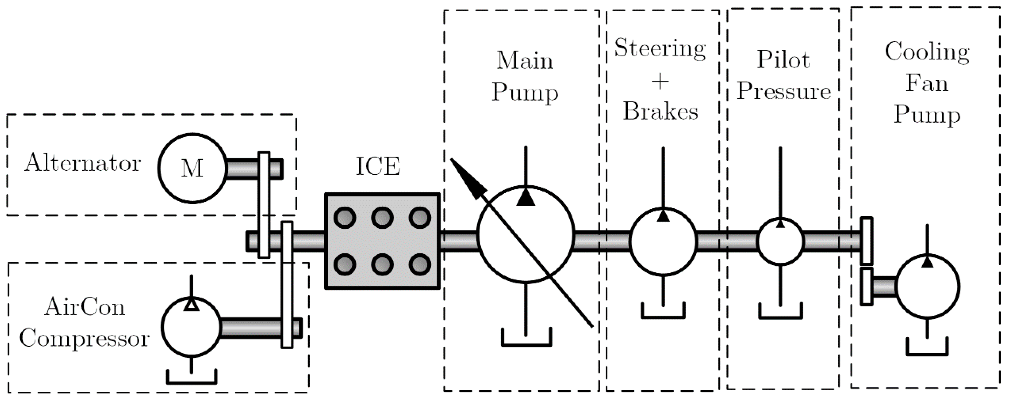
Apart from the hydraulic system, the engine also provides power to a number of smaller subsystems, referred to as ancillary drives, which basically only consume energy and do not directly contribute in the generation of useful work, but without them the machine could not function. A typical setup is shown schematically in Figure 8.
These include:
- The alternator regulating the machine’s 24 V electrical system;
- The air conditioning compressor unit;
- A number of hydraulic gear pumps providing pressure for the joysticks as well as for the steering, braking and cooling systems. It should be noted that crawler type excavators do not have a separate steering system and therefore do not require a pump supplying steering pressure.
Figure 9 shows measurements of engine output power in an excavator at idle for different engine speed settings. To keep all the components on the shaft, including the ancillary drives and main pump, rotating up to 30% of the engine’s full output power is consumed.
In mathematical terms, the idle power demand can be described as a linear function of the engine speed:
In order to ensure no damage occurs if the machine is operated at low speeds, the ancillary drives are dimensioned to be fully functional at lower engine speeds of 800 rpm. Therefore, the additional ancillary power produced at higher engine speeds is totally unnecessary and can be considered as an additional loss term.
3. Cycle Analysis
Hydraulic excavators, especially in the case of those up to 25 tons, are used for a variety of different tasks not only for digging and moving earth. As a result, engineers have to deal with the complex task of having to design a machine without knowledge of its exact future application. Fortunately, collecting detailed information on fuel consumption and other important system states, is becoming easier with the introduction of fleet management systems. These allow companies to track and record the movements as well as operation of all their machines [31]. Without a doubt, this new technology will help change the way machines are designed, as engineers learn how to mine and extract valuable knowledge from these massive data quantities. In 2013, Liebherr published some interesting results for a wheeled excavator obtained using their LiDat system [32]. These showed that the machine spent 25% of its operating time idling, 15% travelling between worksites and the remaining 60% performing actual earth moving tasks. Using a similar fleet management system, researchers in Wuppertal collected data for 3733 machines over a period of six months [33]. For wheeled excavators, they found that, on average, these machines spent 30% of their operating time idling, 20% travelling, 10% grading and 40% digging. Tracked excavators spent 15% at idle, 10% travelling, 15% grading and the remaining 60% of their operating time digging.
3.1. Characteristics of Typical Duty Cycles
Although not exhaustive, a survey of research conducted in this field suggests that dig and dump, trenching, and grading are the three most common duty cycles performed by excavators [21,33]. These are illustrated in Figure 10. An analysis of measurement data, collected from an 18 t excavator performing these three cycles, shows some typical aspects of excavator operation, which can help explain the main cause of losses and identify potential for improvement.
The first important characteristic to take note of is the large fluctuation in actuator power demand for all three cycles. Table 1 summarises these fluctuations using three parameters: describes the ratio of the mean and maximum actuator power demand during the cycle, describes the ratio of the mean and maximum pump flow rate during the cycle and finally describes the ratio of the mean and maximum pump pressure during the cycle. The peak power required for each of the cycles is at least five greater than the mean power output. Similarly, the peak values for the pump flow rate and pressure are approximately two times greater than the mean values.
These observations should come as no surprise because a machine like an excavator can, in fact, only perform cyclic tasks. Every time the boom is raised, it must eventually be lowered. Similarly, every acceleration of the swing drive must be followed by its deceleration. Every period of high power demand is followed by a period in which energy is no longer required or can actually be recovered from the actuator. The only exception to this rule is travelling operation, during which constant power is required for a prolonged period of time. For all other cycles, the power demand will fluctuate considerably.
An important consequence of the fluctuating power is that all the components in the system must be designed for peak requirements but will spend most of their time actually operating at part load. As will be discussed later on in this section, part loading is associated with low efficiency values for both the engine and pump.
The second property, typical for multi-actuator hydraulic systems, is illustrated for each cycle and actuator in Figure 11. Due to the kinematic arrangement of the excavator arm the load force acting on an actuator not only varies during a duty cycle but is also different compared to the load force experienced by the other actuators. This means that each actuator has its own unique power demand profile, which can be expressed in terms of load pressure and required flow rate . As discussed previously, using valves to distribute flow from a single pump to multiple actuators with mismatched power profiles is inefficient.
Before continuing, an important aspect must be mentioned. Yes, for the majority of applications power demand does fluctuate considerably and the average engine output power is lower than its rated power; nevertheless, a machine must be capable of supplying the rated power continuously for prolonged periods of time. For example, when travelling at full speed (30–35 km/h) in a wheeled excavator or for tasks requiring the use of a special attachment like a drill, during which a continuously high pump flow rate is demanded. This must be considered when designing any new system.
3.2. Energy Recovery in Excavators
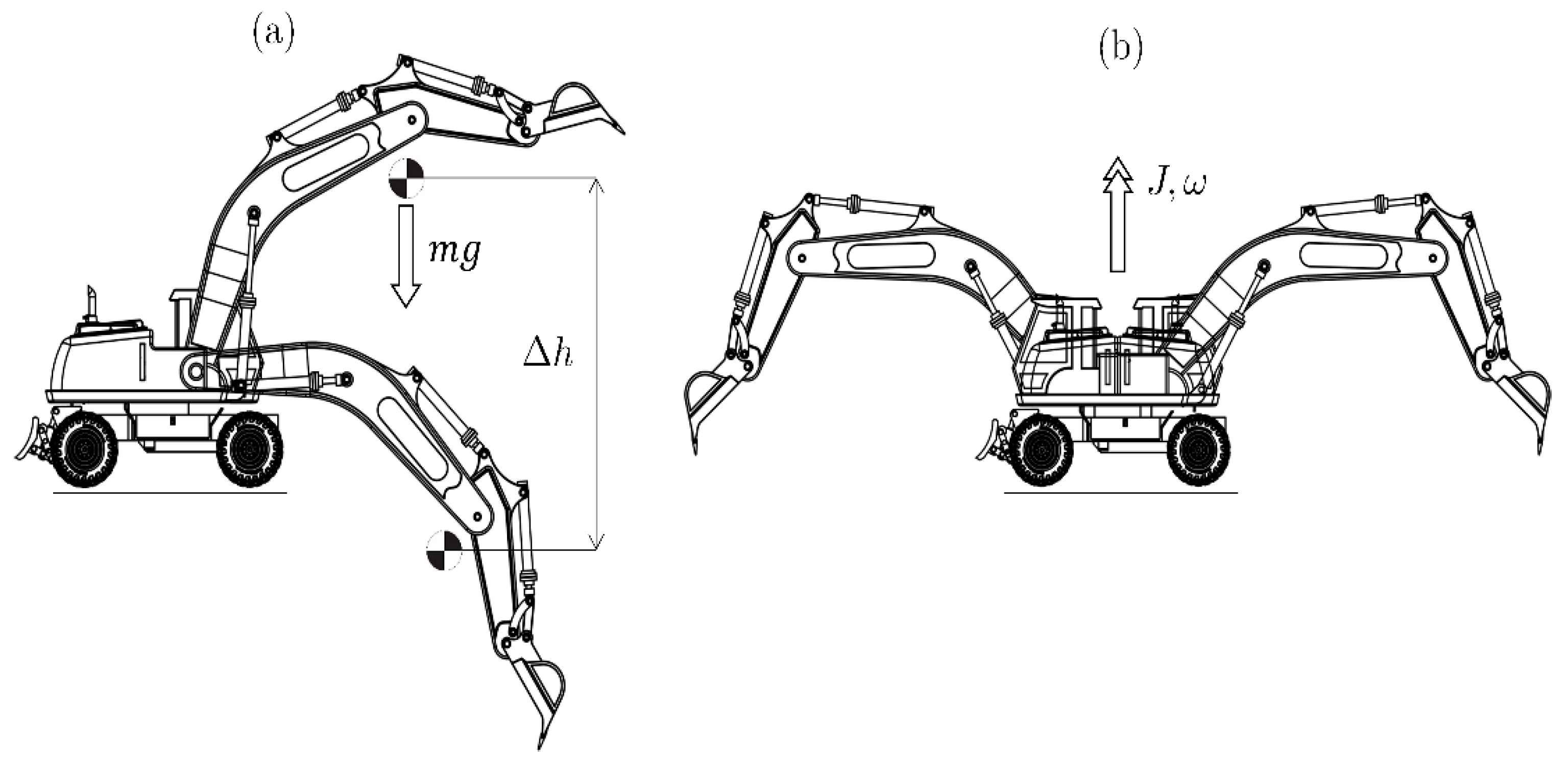
The energy available for recovery in an excavator is found in two forms, either gravitational potential energy or mechanical kinetic energy. When lowering a body of mass m by a distance through a gravitational field of strength g the energy , described by Equation (9), is released. Similarly, when a body, with mass and rotational inertia , traveling at a speed , or rotating at a speed , decelerates its kinetic energy (Equation (10)) is made available.
It is worth taking a moment to appreciate the similarities and differences in these two equations. Both are linearly dependent on the mass or inertia. Similarly, a change in height affects the potential energy linearly, but a change in speed affects the kinetic energy quadratically. Consequently, changes in mass or height have less of an influence compared to changes in speed.
Due to its substantial mass and large changes in height, the boom structure has the greatest amount of recoverable potential energy, Figure 12a. On the other hand, due to the low speed of the centre of mass its kinetic energy is negligible. Similarly, potential energy can be recovered from the arm and bucket actuator, but considerably less compared to the boom. The swing drives possesses no potential energy, but due to its large rotational inertia , a considerable amount of kinetic energy is generated as the superstructure is accelerated (Figure 12b).
If the energy released during lowering and braking cannot be reused immediately or stored, it must be dissipated and leave the system in the form of heat. In a standard valve controlled machine, the recoverable energy is first converted into hydraulic power, in the form of flow Q and pressure p, which is then throttled to tank pressure thereby generating heat and causing an unnecessary increase in oil temperature (Figure 13).
Numerous papers and patents discussing ways to recover boom and swing energy have been published in recent years [34,35,36,37,38,39].
Unfortunately, few of these publications answer the following four fundamental questions:
- Which actuator has the highest amount of recoverable energy?
- Should this energy be stored or can it be reused immediately?
- How difficult, or in other words feasible, is it to recover energy from each of these actuators?
- How much of the energy sent to the various actuators can be recovered?
It is difficult to give a universally valid answer to all four questions. The amount of recoverable energy depends on the duty cycle and the size of the excavator. To accurately determine these quantities it would be necessary to take a range of differently sized machines and conduct extensive tests. Such a study would be invaluable but has yet to be published.
Table 2 summarises measurement data regarding recoverable energy for an 18 t excavator. Four different cycles were analysed. To begin with a simple 90° and then 180° swing acceleration and braking motion, followed by a 90° and 180° dig and dump cycle. The data reveals some interesting facts. During a 90° swing motion, the machine reaches only seventy per cent of the maximum swing rotational speed as the operator is forced to already start braking around the 60° mark in order to come to a stop after 90°. During a 180° motion, the full swing speed is reached. Due to the quadratic relationship between speed and energy (Equation (9)), a 90° rotation has approximately only half as much kinetic energy as a 180° rotation. Furthermore, the potential energy x that can be recovered when lowering the boom in a typical dig and dump cycle (D&D) is twice as large as the kinetic energy of the swing at full speed. Despite this, the swing should not be disregarded because, during each D&D cycle, it is accelerated and decelerated twice while the boom is only lowered once. Therefore, in the case of a 180° D&D cycle, the swing and boom have the same amount of recoverable energy. For the same cycle, measurements show that ten times less energy can be recovered from the arm actuator.
For larger machines the amount of boom and swing energy will increase, but it is difficult to judge how their ratio is affected. In the case of the boom, the weight, mg, and the height, Δh, of the attachment structure increase with the size of the machine. This is not the case for the swing drive as the rotational inertia, J, increases with operating weight but the maximum rotational speed, ω, decreases.
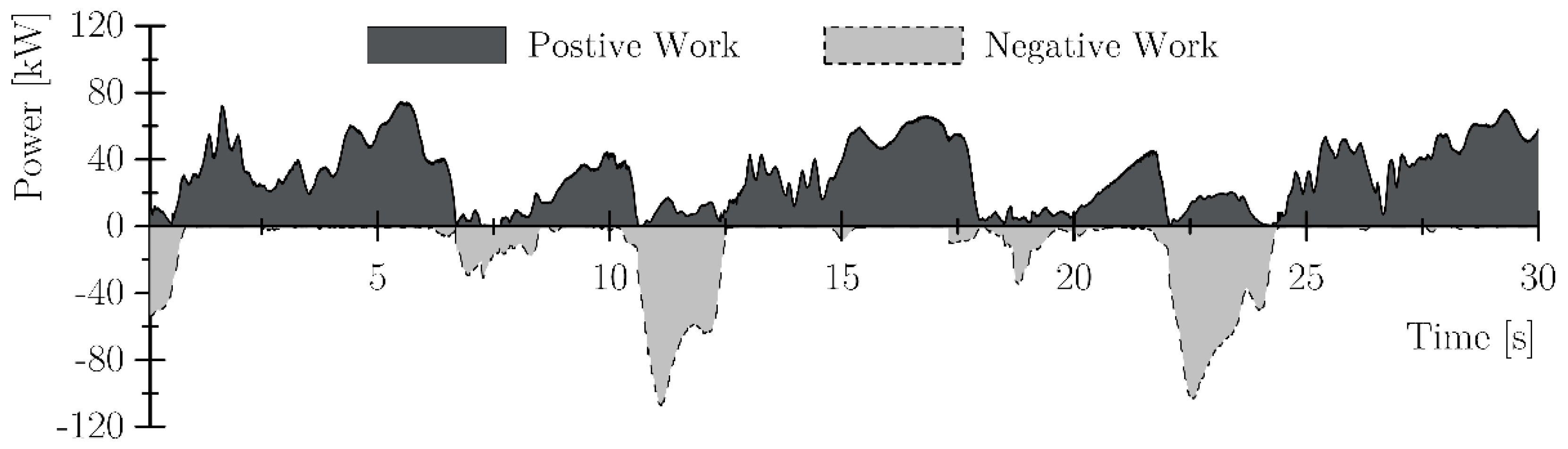
Figure 14 answers the second question. In a D&D cycle, during swing braking and boom lowering no other actuator requires this amount of power at exactly the same moment. Therefore, the only way to take advantage of the recoverable energy is to store it and then reuse it at a later stage. This takes us to the third question, feasibility. In general, storing energy is not a problem, but the ability to reuse it efficiently and cost effectively determines whether recovery is feasible. If the energy is to be stored hydraulically, two factors are important. First, the design and sizing of the storage device is much simpler if the actuator pressure during recovery is fairly constant and known beforehand. Secondly, if the recovery pressure level is greater than the pressure level during the reuse phase, the stored oil can be sent directly to the actuator, making things easier.
This explains why recovering swing energy is feasible. The pressure during braking is not only constant but is also higher than the maximum pressure during acceleration. As a result, brake energy can easily be stored and used to assist the acceleration phase. The boom is far more complex. Due to the kinematic arrangement and wide range of lowering speeds, the pressure level during boom down operation is not constant. Furthermore, the pressure level during boom up operation is usually considerably higher. Consequently, despite the large amount of potential energy that can be recovered, reusing it is far more difficult and costly in comparison to the swing drive.
Finally, to answer the last question, what portion of the energy delivered to the actuator can be recovered? If this ratio is small, then it does not make sense to invest in such technologies. An integration of the areas under the curves in Figure 14 reveals that approximately half of the energy used to accelerate and move the actuators can in fact be recovered. Put differently, if all the energy from the actuators could be recovered and reused without any losses, the engine would only have to supply half as much energy. We can conclude that an excavator is very well suited for systems with integrated recovery circuits.
In summary, the typical operating conditions can be described as follows [40]:
- Average power requirements are considerably lower than peak power requirements.
- Actuator power can be positive (lifting, accelerating) or negative (lowering, decelerating). The peak negative power can reach levels similar to the rated engine power.
- Demand profiles (pressure and flow rate) of all actuators vary independently of each other. Some actuators require high pressure and low flow rate, while others may require a low pressure and high flow rate.
- Idling is common.
Now that the basic concepts regarding how an excavator works and the tasks it performs are clear, a couple of definitions and methods to compare losses can be introduced.
4. Defining Efficiency and Quantifying Losses
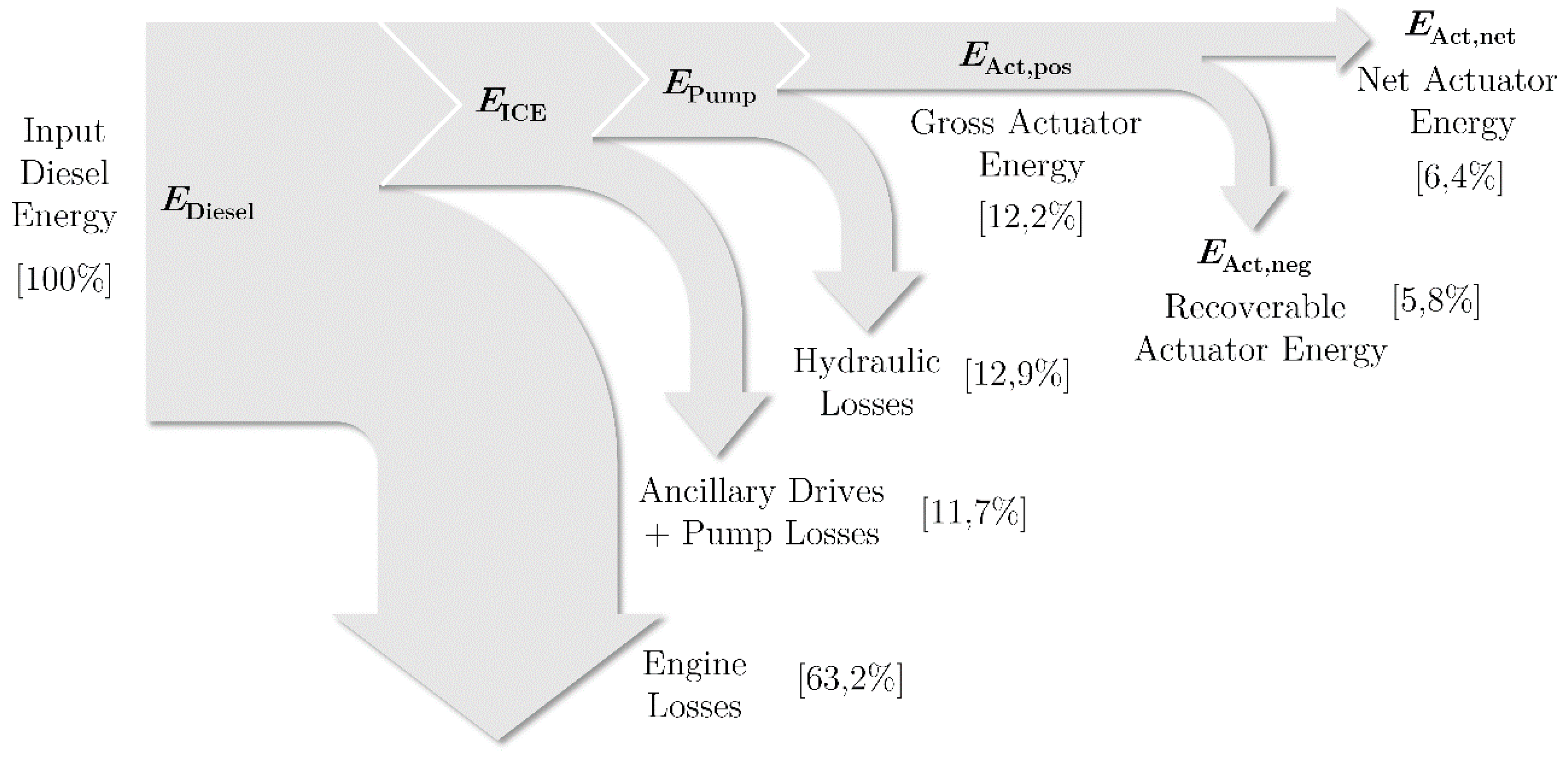
Figure 15 shows a Sankey plot of the energy flow for a 90° dig and dump cycle. The results are comparable with those published by Sturm for a similar machine [25]. As expected, more than 60% of the energy contained in the fuel is lost through the combustion process. A further 11.7% consumed by the ancillary drives and pump. Approximately half the energy supplied by the pump, , is lost through throttling and other hydraulic losses, such as pipe friction. In total, only about 12% of the total input energy is delivered to the actuators, . Half this energy actually performs useful work on the objects in the surroundings, while the other half is used to raise and accelerate the implement structure. Instead of recovering this portion during lowering and braking actions, it is throttled to tank and is dissipated as heat.
In summary, the diagram reveals that approximately a third of the energy supplied by the engine is consumed by the ancillary drives and pump, a third is lost through throttling in the hydraulic system and only the last third actually reaches the actuators.
4.1. System Efficiency
Using the diagram, the hydraulic system efficiency is defined as:
For the dig and dump cycle a hydraulic efficiency of approximately 49% is given, which is actually a very good value for a valve controlled hydraulic system with four actuators and only one supplying pump. The hydraulic system efficiency depends on the number of pumps used in the system and how the valves are used to distribute the flow among the actuator. Consequently, a typical single circuit Load Sensing system has an efficiency of up to 50%, while dual circuit positive control systems can reach efficiencies around 60%.
Total system efficiency can be defined in two different ways. If we are only interested in knowing how much of the fuels energy entering the system, , is actually delivered to the actuators , then the total gross efficiency is the relevant quantity:
If the fact that energy can be recovered and reused is considered, then the total net efficiency is relevant:
Defining system efficiency in these terms conceals the fact that a machine still consumes fuel when just idling because the individual efficiencies would be calculated to 0% with = 0 disregarding the amount of . Instead of discussing efficiencies solely, an evaluation of absolute losses and fuel consumption is more expedient.
4.2. Absolute Losses and Fuel Consumption
A far more useful approximation of a machine’s fuel consumption can be derived by combining the Willans approximation (Equation (1)) with the idle power demand relation (Equation (8)) and the definition of hydraulic efficiency (Equation (11)). Because the idle pump losses are already included in the term , it is necessary to introduce the differential pump efficiency , which describes how much extra engine power must be supplied to the pump to produce additional hydraulic power. Although the pump’s differential efficiency changes slightly depending on the pressure and displacement setting, measurements show that can be roughly approximated using a constant value of 0.9.
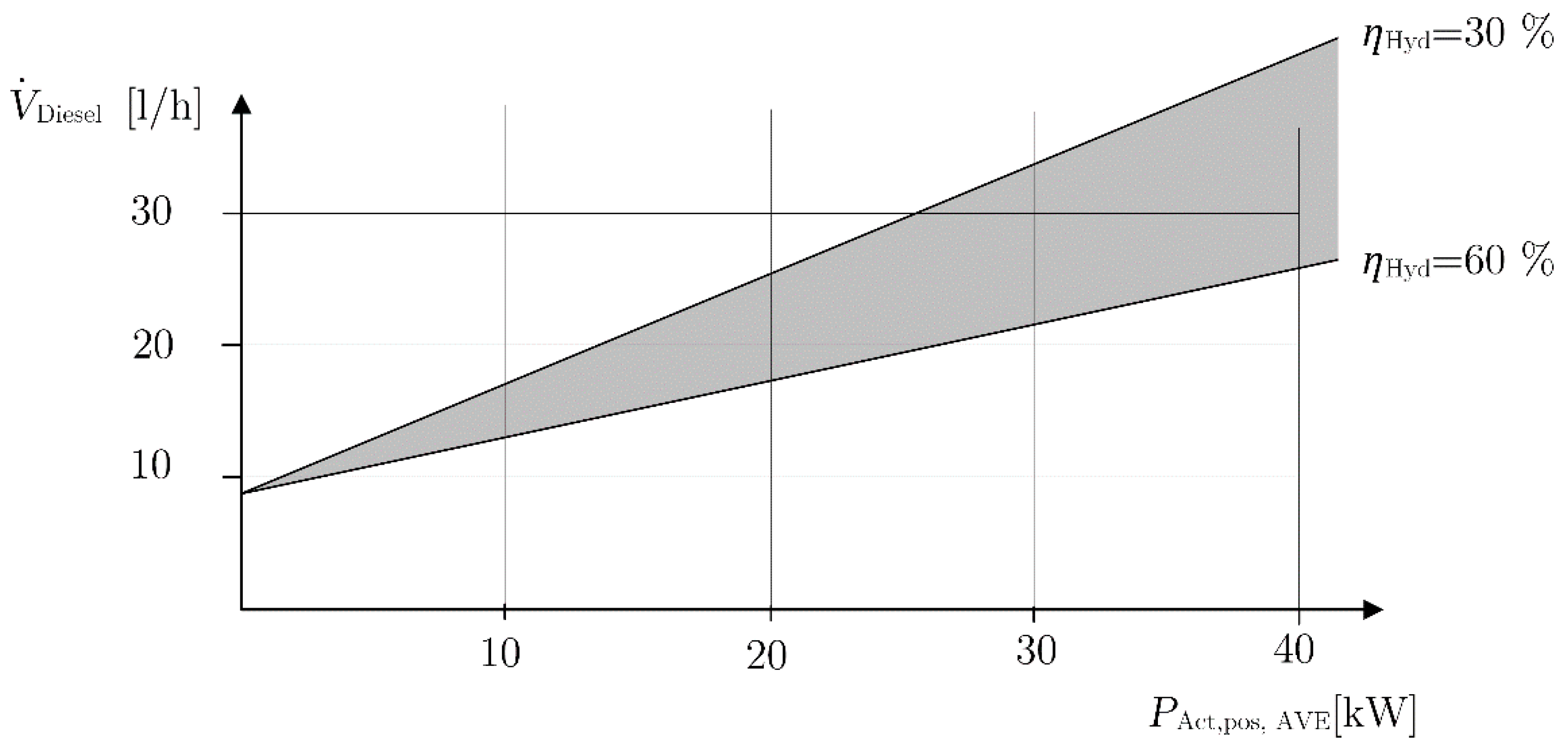
To show how useful the equation is, consider an 18 t excavator with a six-litre diesel engine operating at 1800 rpm as an example. , determined using Equation (2), is approximately 2.9 L/h and a typical value for is 0.0167 kW/rpm. Assuming an average hydraulic system efficiency of between 30% and 60% results in the following relation
Figure 16 shows this inequality graphically.
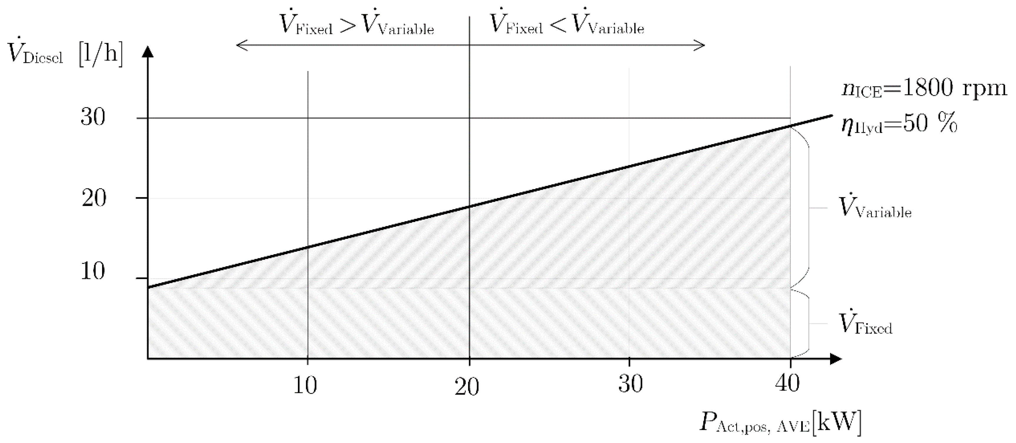
This means that even when just idling and conducting no work, the machine will still consume 9.5 L of fuel per hour. The total amount of fuel consumed due to this phenomenon will be referred to as the fixed fuel consumption .
In the case of a grading cycle with a low average actuator power demand of around 10 kW the fuel consumption only increases by 4.89 L/h compared to idle. This additional amount of fuel consumed to actually perform the cycle will be referred to as the variable fuel consumption . The variable fuel consumption is not affected by the engine operation as the engine’s differential efficiency is constant according to Willans. As shown in Figure 17 only for cycles with average actuator power demands greater than 20 kW does the variable fuel consumption surpass the fixed fuel consumption.
4.3. Model Validation
The very simplified model behind Equations (14) and (15) does not consider dynamic effects as frequent transient loading conditions, which further increase fuel consumption. Despite this, measurements conducted on a real machine correlate well with the predicted theoretical values. Figure 18 proves the good comparability of the measured fuel rate and the introduced fuel consumption model (Equation (14)) with a hydraulic efficiency of 49%, which was calculated for the dig and dump cycle in Section 4.2.
Fuel rate fluctuations around the idealized Willans line are caused by a varying hydraulic efficiency during the cycle and the mentioned transient loading of the engine, whereby more fuel is consumed to prevent the engine from stalling. Averaged values of fuel rate and positive actuator power for the dig and dump cycle were calculated and are also plotted in Figure 18. The low average power demand compared to the maximum power demand becomes apparent. This analysis was done for a variety of different load cycles (see Figure 19).
Most of the cycles reach hydraulic efficiencies in the range of 30–50%. In contrast to that the air grading cycle, which simulates a common grading cycle (cf. Figure 10) but without any external loads, reveals a hydraulic efficiency of 22% and a total gross efficiency of 5%. This result is a direct consequence of the single circuit hydraulic system used in wheeled excavators. At one stage during this cycle the boom is raised and simultaneously the arm cylinder is extended rapidly. Hence the system pressure is set by the boom’s piston pressure, which is considerably higher (approximately 110 bar) than the required pressure to supply the arm cylinder. In combination with a high flow demand of the arm (approximately 200 L/min) throttling losses of about 35 kW can be observed at the inlet edge of the arm control valve. In the case of a real grading cycle the load and accordingly the pressure, which is needed to supply the arm drive, increases leading to lower throttling losses and finally to a higher hydraulic efficiency of 30%. Based on these results, an averaged hydraulic efficiency of 40% is assumed hereafter, see Equation 17.
5. Predicting Fuel Consumption Improvements
Now that the loss mechanisms occurring in an excavator are clear, we can take the next step and consider ways to reduce fuel consumption and to predict the level of improvement with the help of this simple model using Willans lines.
5.1. Saving Fuel by Lowering Hydraulic Losses
The majority of research in the field of energy efficient excavators has dealt with the development of methods to lower hydraulic losses. A number of publications have investigated the ability of different oils to improve hydraulic efficiency [1,41,42]. However, what most of these studies have failed to discuss is the direct impact of these changes to the hydraulic systems on fuel consumption. Using Equation (18), the fuel consumption reduction of a machine operating with a theoretically lossless hydraulic system can be studied:
Figure 20 reveals that even if it were possible to design a system capable of completely eliminating throttling, fuel consumption could be reduced by no more than 30% for a dig and dump cycle.
For other cycles with a lower average positive actuator power this theoretical value is even lower.
A hydraulic circuit capable of reducing throttling losses to a minimum is a displacement controlled system. Instead of using valves to control actuator motion, a single hydraulic unit supplies each actuator with the required power individually. The actuators velocity is controlled by regulating the pump’s displacement. Unfortunately, the considerable higher costs as well as the low system damping associated with these systems have prevented them from being an economic and easy to control alternative to valve controlled systems. Another, more promising, approach to reduce throttling losses is independent metering valves, which decouple the meter in and the meter out edges. As mentioned before the outlet edge is necessary to maintain controllability and even more important to prevent runaway loads. An independently controllable meter out edge enables a reduction of throttling losses to a minimum depending on the actual load pressure of the actuator. With such a system hydraulic efficiencies of about 70% can be achieved. However, as shown in Figure 21, the reduction in fuel consumption for the dig and dump cycle is thereby limited to approximately 17%.
Solutions solely focused on the hydraulic subsystem, without any consideration of the fixed fuel consumption, are therefore very limited.
5.2. Saving Fuel by Lowering Idle Losses
Although it is not often mentioned explicitly, the concept of idle consumption is actually behind many of the fuel saving methods discussed in literature. Engine downspeeding, engine downsizing and start–stop systems all improve machine efficiency by lowering idling losses. Downspeeding not only lowers the friction losses in the engine itself, which are a quadratic function of the speed (Equation (2)), but also lowers the parasitic power demanded by the ancillary drives (Equation (8)). For example, using the same simplified model from above, by reducing engine speed from 1800 rpm down to 1200 rpm, the fuel consumption relation becomes:
Figure 22 shows the relation graphically. Especially for cycles with low average power demands, this measure is very effective, more so than any optimisation of the hydraulic system. The efficiency improvements resulting from downspeeding have been shown in numerous studies [20,43,44]. What these studies have also shown is that a reduced engine speed also lowers productivity because the engine can no longer supply the same amount of power as at the higher speed.
Downsizing, i.e., using a smaller engine with less power, is also discussed frequently, but is very difficult to implement in an excavator. For duty cycles like travelling and drilling with an attachment, in which full power is demanded for prolonged periods of time a downsized engine will just not have the required power. Although these cycles are less frequent than others, the machine must be capable of performing them. Start–stop systems are particularly interesting, as the engine is completely switched off meaning absolutely no fuel is consumed. This is especially efficient for cars in city traffic that are frequently stopping at traffic lights. Implementing this technology in construction machinery is considerably more difficult.
Other methods to lower idle power demand, which are not directly related to the engine, include removing ancillary drives from the engine shaft and using decentralised electric drives, for example for the cooling fan pump.
5.3. Saving Fuel through Energy Recovery
Various methods of recovering and reusing both boom and swing energy have been proposed in literature and can now be found in various series machines available on the market [45]. An important issue to address is the potential of energy recovery methods to lower fuel consumption. To do so the fuel consumption model is extended to include negative actuator power. If a recovery system with an efficiency of were installed the engine would be required to supply less power and the average fuel consumption would be
Measurements show that the average negative actuator power is always less than or equal to 50% of the average positive actuator power. For cycles such as dig and dump the maximum of 50% is reached but in the case of trenching this value goes down to approximately 30%. This can be expressed with the following inequality:
Inserting Equation (20) into Equation (21), assuming a recovery efficiency of 100%, gives the minimum theoretical fuel consumption of a perfect recovery system, capable of recovering boom, swing and arm energy (see Figure 23).
5.4. Saving Fuel through Holistic Approach
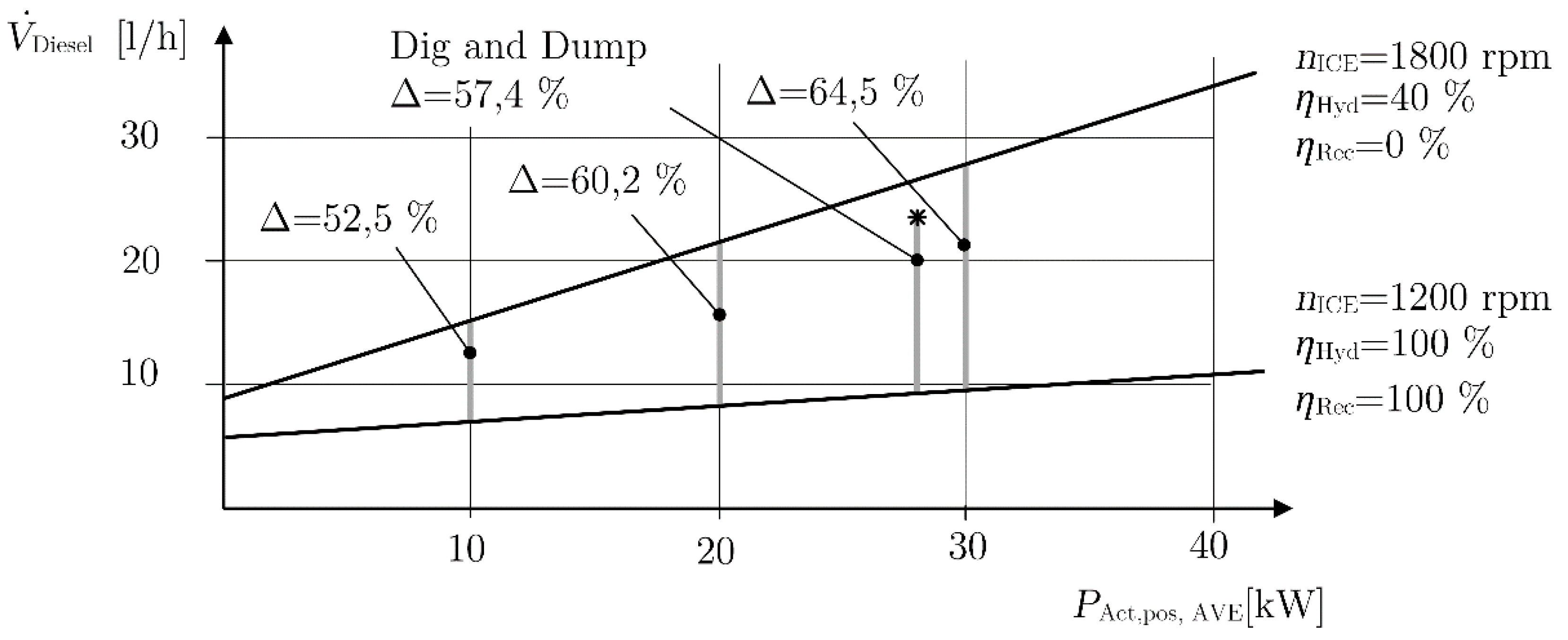
The only way to drastically lower fuel consumption is to follow a holistic approach [40,46]. This means improving the hydraulics, enabling energy recovery and lowering idle fuel consumption. For a machine operating at 1200 rpm, with a lossless hydraulic system and optimal energy recovery, the minimum theoretical fuel consumption can be calculated as follows:
As shown in Figure 24, this results in both a parallel displacement and a change in gradient of the consumption line. Theoretically, consumption can be reduced by up 59% for the dig and dump cycle. In practice, this value cannot be reached but it is helpful to have a theoretical limit.
6. Conclusions
A detailed examination of measurement data shows that the fuel consumption of an excavator can be divided into a fixed and variable component. The fixed component quantifies the amount of fuel the machine consumes if it was just left at idle and did not move for the entire cycle time. The variable component specifies the additional amount of fuel consumed in order to actually perform the task. Depending on the cycle the ratio of fixed to variable fuel consumption changes. In cycles with low average power demands, for example grading, the fixed consumption is actually greater than the variable consumption. Consequently, lowering the total fuel consumption of a machine, requires a consideration of both the fixed and variable terms.
The model introduced in this paper helps assess the potential of certain measures regarding their ability to lower fuel consumption a priori. An interesting result is that a hydraulic system with 100% efficiency can only reduce the fuel consumption during grading by approximately 25%. This is because improvements in the hydraulic system efficiency only lower the variable consumption, not the fixed consumption. Similarly, a machine capable of recovering all available boom potential and swing kinetic energy can theoretically only reduce fuel consumption by a maximum of around 30%. Consequently, thinking only in terms of hydraulic efficiency is rather misleading. A more holistic approach, considering engine operation and other important factors, is far better suited.
Author Contributions
Milos Vukovic and Roland Leifeld performed the measurements and analysed the data. All authors contributed to the writing of the paper.
Conflicts of Interest
The authors declare no conflict of interest.
References
- Abekawa, T.; Tanikawa, Y.; Hirosawa, A. Introduction of Komatsu Genuine Hydraulic Oil KOMHYDRO HE; Komatsu Technical Report; Yumpu: Komatsu, Japan, 2010; Volume 56, No. 163. [Google Scholar]
- Ohira, S.; Suehiro, M.; Ota, K.; Kawamura, K. Use of emission rights for construction machinery to help prevent global warming. Hitachi Rev. 2013, 62, 123–130. [Google Scholar]
- Bloomfield, L.A. How Things Work: The Physics of Everyday Life; John Wiley & Sons: Inc.: Hoboken, NJ, USA, 2013. [Google Scholar]
- Pragmatic Efficiency Limits for Internal Combustion Engines, Readout Guest Forum. 2014. Available online: http://www.horiba.com/publications/readout/article/pragmatic-efficiency-limits-for-internal-combustion-engines-31871/ (accessed on 7 October 2016).
- Hanlon, M. Most Powerful Diesel Engine in the World, Gizmag. Available online: http://www.gizmag.com/go/3263/ (accessed on 7 October 2016).
- Frei, B. Regelung Eines Elektromechanischen Getriebes für Hybridfahrzeuge. Ph.D. Thesis, Technical University Chemnitz, Chemnitz, Germany, 2006. [Google Scholar]
- Yang, J.; Quan, L.; Yang, Y. Excavator energy-saving efficiency based on diesel engine cylinder deactivation technology. Chin. J. Mech. Eng. 2012, 25. [Google Scholar] [CrossRef]
- Liebl, J.; Lederer, M.; Rohde-Brandenburger, K.; Biermann, J.-W.; Roth, M.; Schäfer, H. Energiemanagement im Kraftfahrzeug; Springer: Wiesbaden, Germany, 2014. [Google Scholar]
- Rohde-Brandenburger, K. Was bringen 100 kg Gewichtsreduzierung im Verbrauch? In ATZ; Springer: Wiesbaden, Germany, 2013; Volume 115. [Google Scholar]
- Guzzella, L.; Sciaretta, A. Vehicle Propulsion Systems; Springer: Berlin/Heidelberg, Germany, 2013. [Google Scholar]
- Wilde, A. Eine Modulare Funktionsarchitektur für Adaptives Und Vorausschauendes Energiemanagement in Hybridfahrzeugen. Ph.D. Thesis, Technical University Munich, München, Germany, 2008. [Google Scholar]
- Smil, V. Energy: A Beginner’s Guide; Oneworld Publications: London, UK, 2006. [Google Scholar]
- Chiatti, G.; Chiavola, O.; Falcucci, G. Soot Morphology Effects on DPF Performance; SAE Technical Paper 2009-01-1279; SAE: Warrendale, PA, USA, 2009. [Google Scholar] [CrossRef]
- Falcucci, G. A lumped parameter model for diesel soot morphology evaluation and emission control. Proc. Instit. Mech. Eng. Part D J. Automob. Eng. 2012, 226, 987–998. [Google Scholar] [CrossRef]
- Filla, R. Getting Real about Test Cycles; SAE International Off-Highway Engineering: Warrendale, PA, USA, 2013; ISSN 1528-9702. [Google Scholar]
- Terdich, N. Impact of Electrically Assisted Turbocharging on the Transient Response of an Off-Highway Diesel Engine. Ph.D. Thesis, Imperial College London, London, UK, 2015. [Google Scholar]
- Hanson, P.A.; Lindgren, M.; Nordin, M.; Pettersson, O. A methodology for measuring the effects of transient loads on the fuel efficiency of agricultural tractors. Appl. Eng. Agric. 2003, 19. [Google Scholar] [CrossRef]
- Lindgren, M.; Hansson, P.-A. Effects of transient conditions on exhaust emissions from two non-road diesel engines. Biosyst. Eng. 2004, 87, 57–66. [Google Scholar] [CrossRef]
- Forschungsdialog: Erfolgsprojekt STEAM, O+P Ölhydraulik und Pneumatik 07/08; Vereinigte Fachverlage: Mainz, Germany, 2016.
- Kunze, G.; Göhring, H.; Jacob, K. Baumaschinen: Erdbau-Und Tagesbaumaschinen; Vieweg Verlag: Wiesbaden, Germany, 2002. [Google Scholar]
- Holländer, C. Untersuchungen zur Beurteilung und Optimierung von Baggerhydrauliksystemen. Ph.D. Thesis, TU Braunschweig, Braunschweig, Germany, 1988. [Google Scholar]
- Herfs, W. LUDV-Steuerungen für Bagger. Europäische Mobiltagung, Lohr a. Main, Mannesmann Rexroth AG; Presentation (RD 00 207/10.97); Rexroth: Lohr, Germany, 1997. [Google Scholar]
- N.N. Caterpillar M318D Wheeled Excavator Brochure. Available online: http://www.cat.com/en_US/products/new/equipment/wheel-excavators/wheel-excavators/18115489.html (accessed on 7 October 2016).
- Kawasaki K3VL Axial piston pumps for open circuits in mobile. In Industrial and Marine Applications; Datasheet: Kawasaki, Japan, 2014.
- Sturm, C. Bewertung der Energieeffizienz von Antriebssystemen mobiler Arbeitsmaschinen am Beispiel Bagger. Ph.D. Thesis, Karlsruhe Institute of Technology, Karlsruhe, Germany, 2015. [Google Scholar]
- Vukovic, M.; Sgro, S.; Murrenhoff, H. STEAM—Hydraulic design for engine integration. O + P : Fluidtechnik für den Maschinen- und Anlagenbau 2015, 59. Available online: https://publications.rwth-aachen.de/record/466125 (accessed on 29 March 2017).
- Achten, P. Dynamic high-frequency behaviour of the swash plate in a variable displacement axial piston pump. J. Syst. Control Eng. 2013, 227, 1–12. [Google Scholar] [CrossRef]
- Lux, J.; Murrenhoff, H. Experimental loss analysis of displacement controlled pumps. In Proceedings of the 10th International Fluid Power Conference, Dresden, Germany, 8–10 March 2016. [Google Scholar]
- Zhang, J. Pressure compensated metering valve for EH systems. In Proceedings of the National Conference on Fluid Power, Las Vegas, NV, USA, 12–14 March 2008. [Google Scholar]
- Murrenhoff, H. Servohydraulik—Geregelte Hydraulische Antriebe, 4th ed.; Shaker: Aachen, Germany, 2012. [Google Scholar]
- LiDAT the Complete Comprehensive Data Collection and Tracking System from Liebherr; Liebherr Product Brochure; Liebherr: Kirchdorf, Germany, 2016.
- Bolz, G. Konzepte zur Erhöhung der Energieeffizienz von Mobilbaggern. In Proceedings of the 5th Fachtagung Baumaschinentechnik, Dresden, Germany, 20–21 September 2012. [Google Scholar]
- Fecke, M. Standardisierung definierter Lastzyklen und Messmethoden zur Energieverbrauchsermittlung von Baumaschinen. In Proceedings of the 5th Fachtgaung Baumaschinentechnik, Dresden, Germany, 17–19 September 2015. [Google Scholar]
- Steindorff, K. Energierückgewinnung am Beispiel eines ventilgesteuerten hydraulischen Antriebs. Ph.D. Thesis, TU Braunschweig, Braunschweig, Germany, 2010. [Google Scholar]
- Sgro, S.; Murrenhoff, H. Energierückgewinnungssysteme für Baggerausleger—Eine Systematische Übersicht der Vorhandenen Lösungsmöglichkeiten; O+P 10/2010; Vereinigte Fachverlage: Mainz, Germany, 2010. [Google Scholar]
- Amrhein, J.; Neumann, U. PRB—Regeneration of potential energy while boom-down. In Proceedings of the 8th International Conference on Fluid Power, Dresden, Germany, 26–28 March 2012. [Google Scholar]
- Thompson, B.; Yoon, H.; Kim, J.; Lee, J. Swing Energy Recuperation Scheme for Hydraulic Excavators; SAE Technical Paper 2014-01-2402; SAE: Warrendale, PA, USA, 2014. [Google Scholar] [CrossRef]
- Hießl, A.; Scheidl, R. Energy consumption and efficiency measurements of different excavators—Does hybridization pay? In Proceedings of the ASME/BATH Symposium on Fluid Power and Motion Control, Chicago, IL, USA, 12–14 October 2015. [Google Scholar]
- Joo, C.; Stangl, M. Application of power regenerative boom system to excavator. In Proceedings of the 10th International Conference on Fluid Power, Dresden, Germany, 8–10 March 2016. [Google Scholar]
- Vukovic, M.; Sgro, S.; Murrenhoff, H. STEAM—A holistic approach to designing excavator systems. In Proceedings of the 9th International Fluid Power Conference, Aachen, Germany, 24–26 March 2014. [Google Scholar]
- Korane, K. How Hydraulic Fluids Affect Energy Efficiency, Mobile Hydraulic Tips. Available online: http://www.mobilehydraulictips.com/how-hydraulic-fluids-affect-energy-efficiency/ (accessed on 7 October 2016).
- Michael, P.W.; Mettakadapa, S. Bulk Modulus and Traction Effects in an Axial Piston Pump and a Radial Piston Motor. In Proceedings of the 10th International Fluid Power Conference, Dresden, Germany, 8–10 March 2016. [Google Scholar]
- Forche, J. Antriebsstrangmanagement eines Hydraulikbaggers. Ph.D. Thesis, Technical University Braunschweig, Braunschweig, Germany, 2007. [Google Scholar]
- Ng, F.; Harding, J.A.; Glass, J. An eco-approach to optimise efficiency and productivity of a hydraulic excavator. J. Clean. Prod. 2016, 112, 3966–3976. [Google Scholar] [CrossRef]
- Inderelst, M. Efficiency Improvements in Mobile Hydraulic Systems, Ph.D. Thesis, RWTH Aachen University, Aachen, Germany, 2013. [Google Scholar]
- Leifeld, R.; Vukovic, M.; Murrenhoff, H. Hydraulic hybrid architecture for excavators. ATZoffhighway Worldw. 2016, 9, 44–49. [Google Scholar] [CrossRef]
Figure 1.
Layout of a typical hydraulic excavator.

Figure 2.
The flow of power through the machine and the losses along the path.

Figure 3.
(a) Typical diesel engine efficiency map; and (b) Willans approximation of fuel consumption adapted from [8].
Figure 3.
(a) Typical diesel engine efficiency map; and (b) Willans approximation of fuel consumption adapted from [8].

Figure 4.
Measured engine load and rotation speed during a typical excavator cycle.

Figure 5.
Load quadrants experienced by actuators of the implement system.

Figure 6.
Single Circuit Flow Sharing (SC-FS) circuit used in European wheeled excavators, including downstream pressure compensators (PCs) for load independent control, a torque controlled (TC) swing with upstream compensation and LS-pressure bypass on the boom (LSB).
Figure 6.
Single Circuit Flow Sharing (SC-FS) circuit used in European wheeled excavators, including downstream pressure compensators (PCs) for load independent control, a torque controlled (TC) swing with upstream compensation and LS-pressure bypass on the boom (LSB).

Figure 7.
(a) Characteristic efficiency map for a 200 cc axial piston unit [24]; and (b) a schematic of a pump with a load sensing pressure controller.
Figure 7.
(a) Characteristic efficiency map for a 200 cc axial piston unit [24]; and (b) a schematic of a pump with a load sensing pressure controller.

Figure 8.
Ancillary drives in a wheeled excavator.

Figure 9.
Measured engine load and rotation speed during a typical excavator cycle.

Figure 10.
Typical excavator duty cycle.

Figure 11.
Load pressure over flow required for each actuator and cycle.

Figure 12.
(a) Boom potential energy; and (b) swing kinetic energy.

Figure 13.
(a) Energy dissipation during: boom lowering; and (b) swing braking.

Figure 14.
Positive and negative work during dig and dump cycle.

Figure 15.
Sankey plot of energy flow through an 18 t excavator during 90° dig and dump.

Figure 16.
Fuel consumption model (engine speed 1800 rpm).

Figure 17.
Concept of fixed and variable fuel consumption.

Figure 18.
Measurements of load sensing (LS) system compared to fuel consumption model.

Figure 19.
Validation of fuel consumption model.

Figure 20.
Maximum theoretical fuel consumption reduction with a lossless hydraulic system.

Figure 21.
Theoretical fuel consumption reduction of a hydraulic system with 70% efficiency.

Figure 22.
Theoretical fuel consumption reduction possible with engine downspeeding.

Figure 23.
Maximum theoretical fuel consumption reduction possible with energy recovery.

Figure 24.
Maximum theoretical fuel consumption reduction using engine downspeeding, lossless hydraulics and energy recovery.
Figure 24.
Maximum theoretical fuel consumption reduction using engine downspeeding, lossless hydraulics and energy recovery.


Table 1.
Comparison of average and maximum power, flow and pressure for each cycle.
| Cycle | |||
|---|---|---|---|
| Dig & Dump | 0.20 | 0.60 | 0.51 |
| Trenching | 0.18 | 0.50 | 0.50 |
| Grading | 0.08 | 0.45 | 0.44 |
Table 2.
Recoverable actuator energy for an 18 t excavator for various duty cycles compared to the recoverable energy x of the boom drive in a typical dig and dump cycle.
Table 2.
Recoverable actuator energy for an 18 t excavator for various duty cycles compared to the recoverable energy x of the boom drive in a typical dig and dump cycle.
| Swing 90° | Swing 180° | Boom D&D | Arm D&D | Swing 90° D&D | Swing 180° D&D |
|---|---|---|---|---|---|
| 0.25 x | 0.5 x | x | 0.1 x | 0.5 x | x |
© 2017 by the authors. Licensee MDPI, Basel, Switzerland. This article is an open access article distributed under the terms and conditions of the Creative Commons Attribution (CC BY) license (http://creativecommons.org/licenses/by/4.0/).
Share and Cite
MDPI and ACS Style
Vukovic, M.; Leifeld, R.; Murrenhoff, H. Reducing Fuel Consumption in Hydraulic Excavators—A Comprehensive Analysis. Energies 2017, 10, 687. https://doi.org/10.3390/en10050687
AMA Style
Vukovic M, Leifeld R, Murrenhoff H. Reducing Fuel Consumption in Hydraulic Excavators—A Comprehensive Analysis. Energies. 2017; 10(5):687. https://doi.org/10.3390/en10050687
Chicago/Turabian StyleVukovic, Milos, Roland Leifeld, and Hubertus Murrenhoff. 2017. "Reducing Fuel Consumption in Hydraulic Excavators—A Comprehensive Analysis" Energies 10, no. 5: 687. https://doi.org/10.3390/en10050687
Note that from the first issue of 2016, this journal uses article numbers instead of page numbers. See further details here.