
Hybrid Photovoltaic Systems with Accumulation—Support for Electric Vehicle Charging


1
Department of Electrical Power Engineering, Brno University of Technology, Technicka 12, Brno 61600, Czech Republic
2
Department of Electric Power Engineering, Technical University of Košice, Mäsiarska 74, Košice 04001, Slovakia
*
Author to whom correspondence should be addressed.
Energies 2017, 10(7), 834; https://doi.org/10.3390/en10070834
Submission received: 27 April 2017
/
Revised: 7 June 2017
/
Accepted: 16 June 2017
/
Published: 22 June 2017
(This article belongs to the Special Issue Energy Management, Control, and System Architectures for Electric Vehicle Applications)
Abstract
:The paper presents the concept of a hybrid power system with additional energy storage to support electric vehicles (EVs) charging stations. The aim is to verify the possibilities of mutual cooperation of individual elements of the system from the point of view of energy balances and to show possibilities of utilization of accumulation for these purposes using mathematical modeling. The description of the technical solution of the concept is described by a mathematical model in the Matlab Simulink programming environment. Individual elements of the assembled model are described in detail, together with the algorithm of the control logic of charging the supporting storage system. The resulting model was validated via an actual small-scale hybrid system (HS). Within the outputs of the mathematical model, two simulation scenarios are presented, with the aid of which the benefits of the concept presented were verified.
1. Introduction
The current developments in the situation regarding the renewable energy sources (RESs) in the Czech Republic (CR), where after the boom in photovoltaic systems (PVSs) in 2009–2012 the state-subsidized purchase of energy from this source began to be cut back in 2014, are responsible for the change in the target orientation of the market demand. One of the potential development strategies consists in exploiting decentralized energy sources that will be made use of in the area of family houses and office buildings, with focus on maximizing the consumption of generated energy on site, with minimum overflows into the distribution network, if possible.
Decree No 16/2016 of the Czech Energy Regulatory Office about conditions for connection to the public electricity grid defines the simplified conditions for connecting the applicant’s microsource to the distribution system as follows: “an impedance value measured at the point of connection to the distribution system that does not exceed the limit impedance” [1] and the requirement “a technical solution of the microsource that prevents supplying electricity into the distribution system at the point of connection, except for short-term electricity overflows into the distribution system which serve the reaction of the limiting device but which do not increase the voltage value at the connection point” [1].
The trend from the preceding years, when the priority in PVS was to supply energy into the distribution system, has thus changed, together with changes in the legislation and the elimination of subsidies. At present, the main attention is focused on hybrid systems (HSs) with storage of electric/thermal energy [2]. The main advantage of HSs with RESs lies in increased energy self-reliance and reduced dependence on the distribution system. Employing these systems can lead to reduced line loading (reduced transmission losses), postponed investment in the development and maintenance of the electricity grid (EG). With an optimally set power management of HS, all the generated energy or its substantial part can be consumed directly in the given object while minimizing the negative effects on the distribution system [3,4].
The need to reduce the power taken from the grid is, among other things, related to the expected development of electromobility. In spite of the fact that the development of electromobility is still hindered by the state of technology and insufficient infrastructure, electromobility remains a priority, both on the European and the Czech level, in particular from the viewpoint of long-term development in this field (the ever stricter CO2 emission limits on vehicles imposed in EU are the main driving force in this sector). A dynamic growth in the area of alternative drives/fuels can today be witnessed in Compressed Natural Gas (CNG) and electric vehicles. Contemporary developmental trends indicate that CNG will be increasing its share in the market but cannot be expected to become one of the principal fuels. This assumption is based on the lower potential of CNG as regards the reduction of CO2. The development of electromobility in the CR is hindered by several factors such as limited supply of electric vehicles, low number of charging stations or limited customer experience.
According to the Automotive Industry Association (AIA), a total of 2440 electric vehicles were in operation in CR on 1 January 2016. Out of them, a mere 790 were electric cars (according to the latest data there were 992 electric vehicles registered in CR towards the end of 2016), 59 electric trucks, 81 electric industrial vehicles. A full 1495 pieces were electric motorcycles (electric scooters) and three-wheelers [5].
In view of the fact that the driving range of EVs is limited (usually only up to 250 km) and depends, above all, on the accumulator capacity and particular utilization (partially on climatic conditions too) it is necessary to ensure that they are charged up such that they can meet the user’s needs and requirements. It is usual for EVs to be charged in the evening or at night so that in the morning they are operation-ready with full capacity.
For regular charging (up to 7.4 kW), the manufacturers install an accumulator charger directly in EVs. A cable is used for connection to 230 V AC mains. For faster charging (22 kW or 43 kW and more) the manufacturers have chosen two alternative charging versions in compliance with the IEC 61851 Standard [6]:
- Application of integrated charger for charging with 3–43 kW power, with one-phase or three-phase connection.
- Application of an external charger which rectifies alternating current and charges EVs with a power of 50 kW or more.
In any case, expanding the number of charging stations places additional requirements on both the amount of consumed energy and the level of reserved input power which is related to the fast high-power charging stations.
In their basic version, charging stations for electric vehicles employ feeding from the electricity grid, as shown in Figure 1. Another potential technical solution of feeding the charging station is to use a system with RES (PVS, wind turbine), either as a separate or as a cooperating (bivalent) source. Such a concept of the solution leads to setting up a hybrid energy system with a complex energy management that allows maximizing the exploitation of individual energy sources.
Hybrid Energy Systems–State of the Art
Hybrid energy systems have recently undergone a considerable evolution. Initially, separate systems were only concerned (e.g., PVSs with storage) or combinations of alternative energy sources with fossil fuel sources (e.g., combinations of photovoltaic (PV) panels or wind turbines with diesel generator). In the next stage, there appeared combinations of PV panels directly with a wind turbine, supplemented with a storage element [7]. This element can be some kind of accumulator; currently the most frequently used is the lead-acid accumulator (mainly for economic reasons) but the Li-Ion and LiFePO4 technologies have recently been on the increase. Further storage possibilities can be seen, for example, in storing energy in a hydrogen storage and subsequent conversion via fuel cells or in accumulators of the type of Vanadium Redox Battery (VRB) [8].
Employing a storage element is the basic premise for a self-reliant hybrid energy system. The key parameters are:
- Capacity of the storage system.
- Chosen technology.
- Method of operation—depth of discharge and cycling.
An optimally designed storage system can increase the effectiveness of exploiting the energy generated from renewable sources, move the energy consumption peaks to a more appropriate area of the consumption diagram and thus limit the negative effects on the grid (line voltage fluctuation, asymmetry, harmonic distortion,…) [9].
2. Concept of Proposed Solution
In connection with the trend of electromobility development in CR and the related development of charging stations, the concept has been proposed of a HS with supporting storage which is used to ensure the feeding of EV charging stations [10].
With regard to the solar and wind conditions in CR, it can be said that in our conditions it is only the PVSs that can be used for a potential exploitation of RES as a bivalent charging source in a charging station. Excluding the wind energy from the concept of RES cooperating with the charging station is based on the unsatisfactory weather conditions on the territory of CR. In view of the required average wind velocity in excess of 5 m·s−1 at the installation site, the exploitation of this kind of energy would be a considerable limiting factor when localizing individual charging stations.
The proposed concept (Figure 2) has been broadened to include a PV source (yellow arrows) and the resulting solution conception starts from the assumed exploitation of a HS for the feeding of charging stations. Primary use is made of energy from the storage system (green arrows) while the grid is used, above all, in support of charging up the storage system (red arrows). The chosen conception is based on the assumption that most of the energy needed to charge up EVs will be drawn in the low-tariff (LT) period, i.e., it will be stored into accumulation during this period and then utilized as necessary during the day in high-tariff (HT). Energy in the accumulator for EVs can also be used in periods of higher grid loading, which will relieve EG and thus reduce losses related to electricity transmission.
For the purpose of checking the energy balance of the designed system, the operating states of integrated accumulation and the effect of the power parameters of individual subsystems, a simulation model was made in the Matlab Simulink programming environment, which was subsequently validated on a laboratory HS, using data from real measurement.
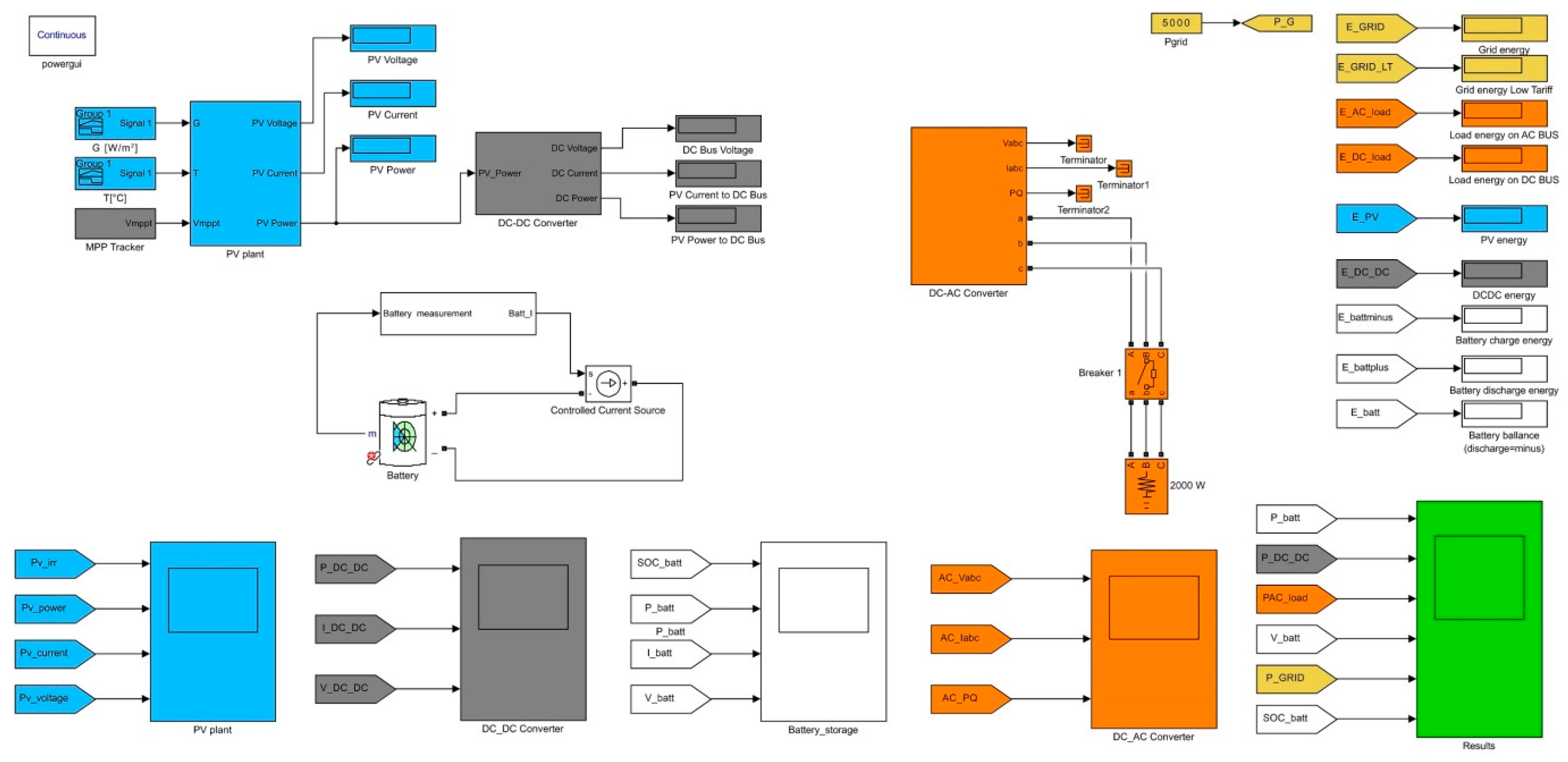
3. Description of Mathematical Model
The HS model was made in the Matlab Simulink programming environment (Figure 3), using elements of the SimPowerSystems library. The model allows predicting not only the energy and power balances of the whole system but also the behaviour of its individual parts. The system is formed by the PV field connected to the DC bus-bar via a DC-DC converter, storage system, DC-AC inverter, and load. In addition to blocks that simulate these physical elements, the model also contains display and calculation blocks for graphic representation of the results of simulated scenarios. After the model was made, its validation was performed; it consisted in comparing the results with measured data on the experimental HS in Brno University of Technology, Faculty of Electrical Engineering and Communication (FEEC BUT) laboratories.
3.1. Photovoltaic Panel
In the PV power plant, the basic energy source is the PV panel made up of series-interconnected individual cells. The PV panel is modelled on the basis of a general one-diode equivalent circuit (Figure 4). A detailed description and the possibilities of determining equivalent parameters are thoroughly discussed in [11,12,13,14,15].
The output current from the PV panel can be described by Equation (1):
where:
- Ipv
- is the input current of PV panel (A),
- Iph
- is the current generated by photodiode (A),
- Is
- is the saturation current (A),
- q
- is the electron charge (q = 1.602 × 10⁻⁹ C),
- V
- is the output voltage of panel (V),
- Ns
- is the number of panel cells in series (-),
- k
- is the Boltzmann constant (k = 1.38 × 10⁻²³ J·K−1),
- T
- is the cell temperature (K),
- A
- is the diode ideality factor (-),
- Rs
- is the series resistance of panel (Ω),
- Rsh
- is the shunt resistance of panel (Ω).
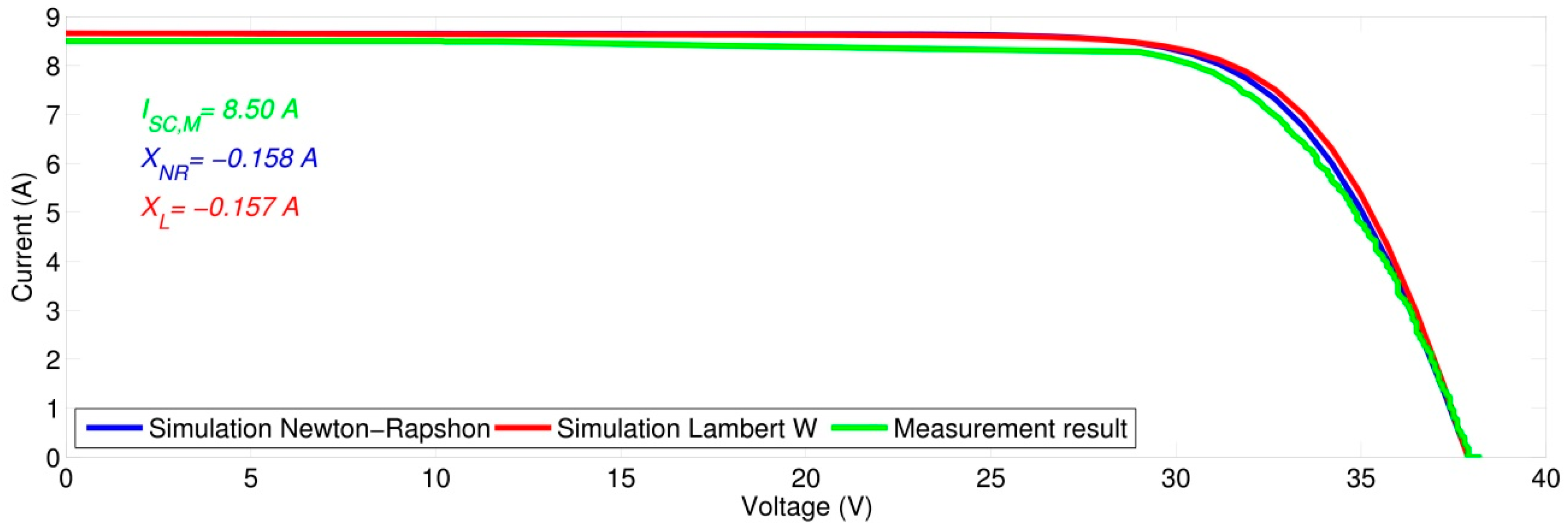
The parameters Rs and Rsh can be determined analytically (on the assumption of choosing the parameter A) from the values given in the data sheet for the particular panel, using the Lambert W function [11]. Another possibility of determining the required parameters is the application of the numerical Newton-Raphson iteration method [15]. In this case it is not necessary to choose the parameter A but the method is strongly dependent on the chosen initial approximation. In case the initial condition is not chosen suitably, divergence will occur in the calculation. The PV panel parameters considered for the simulation are given in Table 1.
A comparison of the results of model simulation with the measurement performed on a physical panel can be seen on the shape of I-V curve (Figure 5). In the region of short-circuit current, the deviation (XNR, XL) of the measured values (ISC,M) from the simulated ones is due to the overall impurity shading of the panel during measurement, which shows in the decreased value of short-circuit current against the value given in the manufacturer’s datasheet. As is obvious from Figure 5, the differences between the results for simulated panel values and the parameters obtained using the Newton-Raphson iteration method and the Lambert W function are minimal and they can be used to determine the required parameters (A, Rs and Rsh).
Other input parameters are the panel temperature t (°C), intensity of solar radiation G in the panel plane (W·m−2) and the particular voltage on the panel output, i.e., the reference voltage Vref determined by the maximum power point tracker (MPPT).
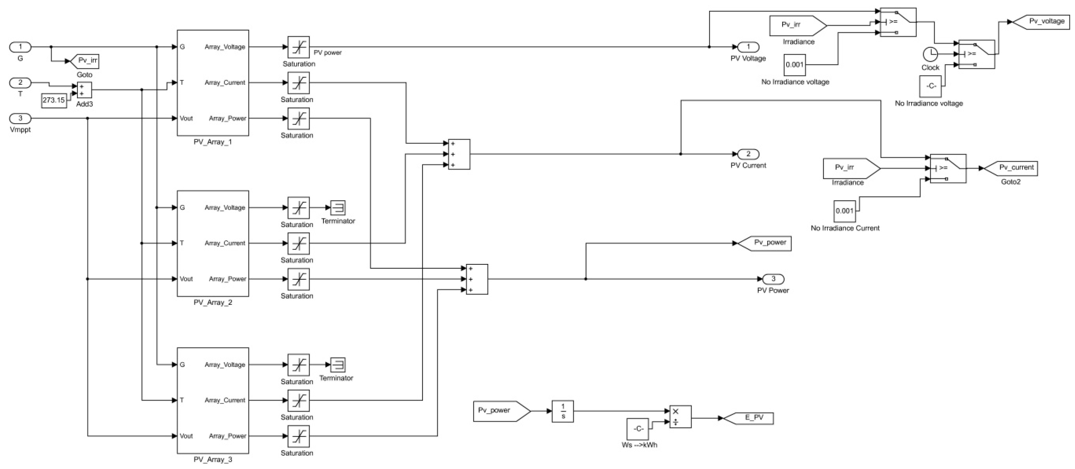
For the PV panel and for individual strings, a mask was prepared in the model that enables changing the input parameters and the connection configuration. The PV field is then formed via a series-parallel interconnection of panels (always according to the requirements on the system’s voltage and current.
The modelled system used in the validation was formed be three parallel-interconnected strings (Figure 6). Each string consists of three series-interconnected panels. In the validation, the panels were oriented towards south at a slope of 35°. Input values for the simulation (daily profile of solar radiation intensity and panel temperatures) correspond directly to the particular orientation.
3.2. DC-DC Converter
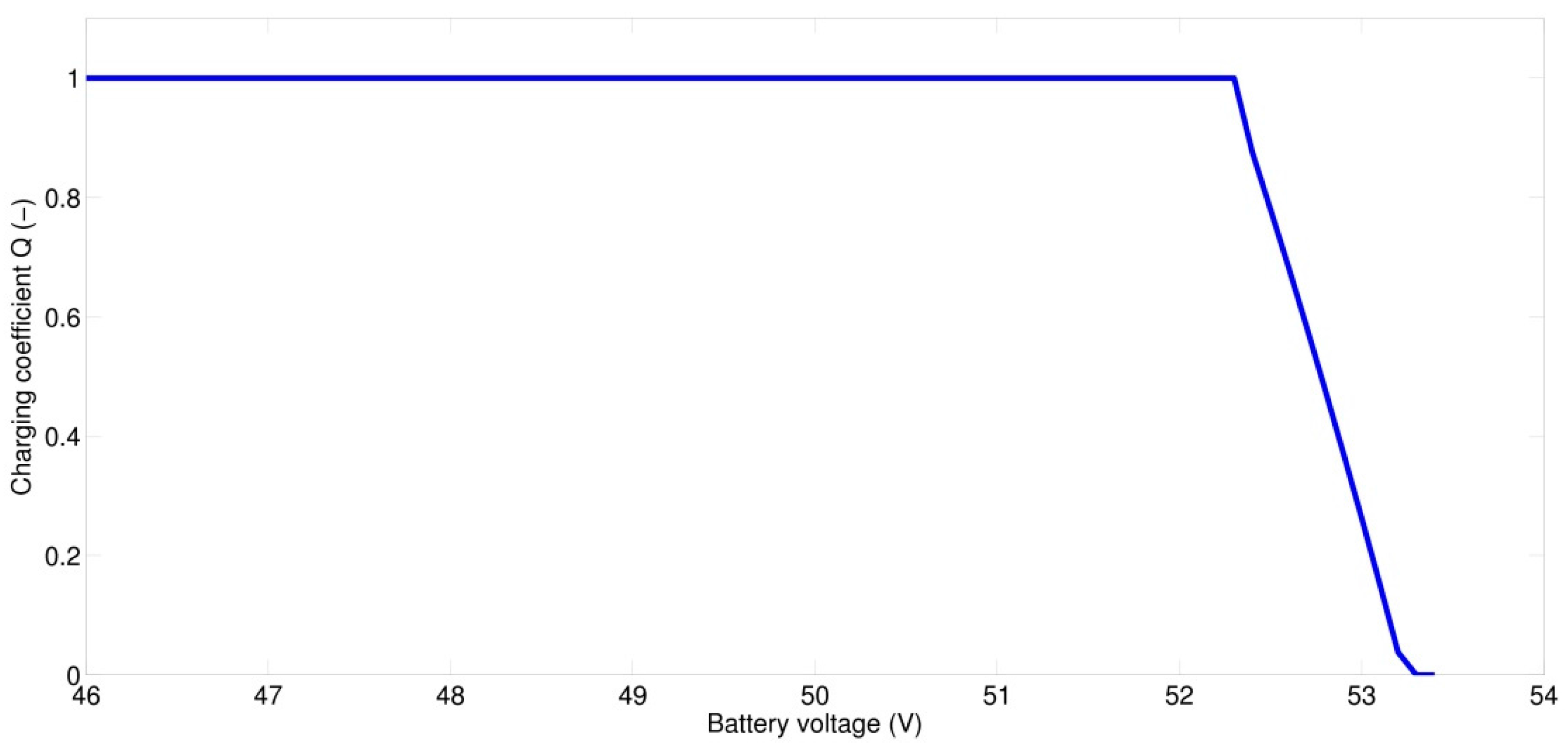
The block which simulates the behaviour of a DC-DC controller was only modelled from the viewpoint of power flow and the respective control functions; switching processes and transient events were not considered. The input value for the block is the output power of PV field. This power is subsequently multiplied by the control coefficient Q, which respects the current state of accumulation and, depending on the particular voltage of the storage system, controls charging power in the range of 0–100%. The dependence of the control coefficient on the accumulation voltage (Figure 7) was determined experimentally, it does not fully respect the charging cycle of the DC-DC controller, which may consist of several different phases for the purpose of optimizing the accumulator lifetime. But for the description of the system’s energy behaviour in the course of a day this dependence is sufficient. In the next step, the constant converter efficiency ηDC-DC = 96% is considered.
Using the current value of accumulation voltage, the controller output current is then calculated from the output power of the DC-DC controller and employed to charge the accumulator or supply the connected load. Within the frame of the controller model the threshold value of the input power is then defined at which the controller starts working. In the model validation this value was found to be 80 W. The behaviour of a DC-DC controller can mathematically be described with the aid of Equations (2) and (3):
where:
- Pin,DC-DC
- is the controller input power (W), i.e., the output power of PV field Pout,PV (W),
- Pout,DC-DC
- is the output power of DC-DC controller (W),
- Q
- is the control coefficient (-).
In addition to the above functions, the DC-DC controller contains the function for tracking the maximum power point of the PV field (MPPT) for the purpose of achieving higher operating efficiency. Because of the climatic dependence of the parameters that describe the pattern of the I-V curve, the maximum power point (MPP) is constantly changing and at any time there is a voltage value Vref, i.e., PV field loading, at which the maximum power can be drawn [13,14]. This fact is the consequence of the non-linearity of the I-V curve. Present-day algorithms for finding MPP differ mostly in the speed and accuracy of finding MPP and also in the demands made on the implementation. The tracking algorithms can generally be divided into three types: Perturb and Observe (P&O), incremental conductance (IC) and Temperature gradient techniques, the first two being the most widely used [16,17,18].
In the assembled model the Perturb and Observe (P&O) method is selected. Operating voltage on the primary side of the controller (power point of PV field) changes in certain fixed steps and the respective change in output power is registered. In case the power increases due to the change in voltage, the controller continues changing the voltage with the same sign. If due to the change in voltage there is a drop in power, in the next step there will be a change in voltage with opposite sign.
The main disadvantage of this method consists in the power point oscillating around the MPP value, a consequence of which is the loss of a small amount of energy due to inaccurate setting [19]. The oscillations correspond to the size of the step in which the change in voltage is made. The accuracy of setting the power point can be increased by reducing the voltage step but at the expense of the speed of search algorithm. This disadvantage manifests itself, above all, when meteorological conditions are changing rapidly. As regards our model, the voltage step was set at the value ΔV = 1 V.
The flow chart giving the essence of the P&O method is shown in Figure 8. Due to the fact that the MPPT is implemented in the model, the simulation step was set to 1 s. With the use of the MPPT, the maximum output power of the PV system is always ensured. The maximum available energy from the PV system (E_PV) is calculated in the model, and this value represents the energy potential of the PV array. The difference between this energy (E_PV) and the energy at the controller output (E_DC_DC, sim) does not indicate a physical energy loss on the DC-DC converter. This is an unused energy that cannot be delivered to the system due to the battery voltage limits.
3.3. Battery Energy Storage and Control System
For the simulation of the storage system the accumulator model from the SimPower Systems library was used, which represents the parameterized model of the common accumulator. The simulation is based on the principle of controlled voltage source with internal resistance.
For model purposes and in connection with the battery used, it was necessary to define the system states and thus describe the behaviour of the hybrid state—its internal logic, so that it would be clearly defined under what circumstances and priorities energy can be fed into or drawn from the battery. The algorithm of the control logic of the system is shown in Figure 9, where the meaning of individual quantities is as follows:
- Pout,DC-DC
- is the output power from DC-DC converter (W),
- Pload,DC
- is the input power into DC-AC inverter for load feeding (W),
- SOCbatt
- is the state of battery charging (%),
- Pbatt
- is the power on accumulator interface–positive value means battery discharging (W),
- Pgrid, LT
- is the power drawn from grid in LT periods (W),
- Pgrid, HT
- is the power drawn from grid in HT periods (W).
Constructing the control logic algorithm was based on the following principal assumptions:
- The system will primarily use the available power Pout, DC-DC to charge the battery and feed the load Pload,DC.
- In the case the SOCbatt drops below the value of 20% and the load power Pload,DC exceeds the available power Pout,DC-DC, the system is charged up from the grid by a constant power Pgrid, which is an optional simulation parameter.
- In HT periods, the power drawn is registered as Pgrid,HT and the charging stops when the limit of 30% SOCbatt is reached.
- In LT periods, charging begins independently of the value of SOCbatt. Power from the grid is registered as Pgrid,LT and charging only stops when the limit of 100% SOCbatt is reached.
Power drawn from the grid is continuously integrated and the result saved in two separate variables in dependence on the currently valid tariff. This provides for separate monitoring of the amount of electric energy drawn in the HT (E_GRID_HT) and LT (E_GRID LT) periods.
3.4. DC-AC Inverter
The inverter function (the inverter itself) in the assembled model can be defined as a device that inverts dc energy to ac energy at a given constant efficiency. Thus the input quantity is the power Pload,DC and the output quantity is the power Pload,AC. In practical applications, the converter efficiency changes in dependence on the current load; for the assembled model the DC-AC inverter efficiency was at ηDC-AC = 95%. The simulation block is formed by a three-phase voltage source which generates voltage for the connected load and is supplemented with voltage and current measuring blocks. Similar to the DC-DC converter, no switching processes were considered.
3.5. Load
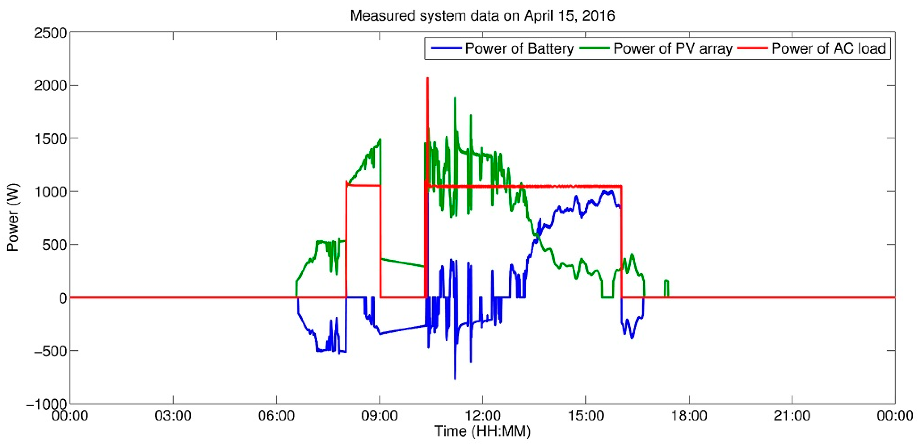
The model offers two possibilities of making a load diagram. The load development can be defined with the aid of several electrical devices being time-switched. This method is implemented using three-phase RLC (Resistor-Inductor-Capacitor) blocks and elements for load switching. The drawn power is measured and entered into the system’s control logic. The other possibility is the direct loading of the required variable, for example via importing the measured or calculated values. For the purpose of simulation, the latter method was used: the load diagram is known in advance and enters the model as an input variable. The load profile for the validation is given in Figure 10 (red curve).
4. Validation of Assembled Model
The functionality and internal logic of the model assembled were validated using data that were measured on the experimental HS in the laboratories of the Department of Electrical Power Engineering (Brno University of Technology, Brno-střed, Czech Republic). A 3390-10 power analyser (Hioki, Nagano, Japan) was used for the measurement conducted on 15 April 2016. Currents were measured using current sensors as follows:
- AC current on the DC-AC inverter output, using the Hioki 9272-10 clamp probe, range 20 A.
- DC current on the DC-DC controller output, using the Hioki 3274 clamp probe, range 150 A.
- DC current on accumulator interface, using the Hioki 9709 pull-through sensor, range 500 A.
Voltage was measured directly, via voltage inputs on the analyser. The mean values of individual measured quantities were registered every 30 s, which from the viewpoint of the validation of energy flows represents sufficient accuracy. The chosen sampling rate is not suitable for the recording of transient events and the model was neither assembled nor validated for the simulation of transient events.
The laboratory system (Figure 11) is formed by a PV array with a power of 2.25 kWp, consisting of nine panels with a power of 250 Wp, interconnected in three parallel-connected strings, each with three panels in series. The accumulator system is made up of lead-acid accumulators with a nominal voltage of 48V and a capacity of 400 Ah. The power section contains two Xtender inverters (Studer Sion, Switzerland), working in the Master-Slave mode to reduce stand-by losses), each of a nominal power of 2600 W (the complete system is described in detail in [20]).
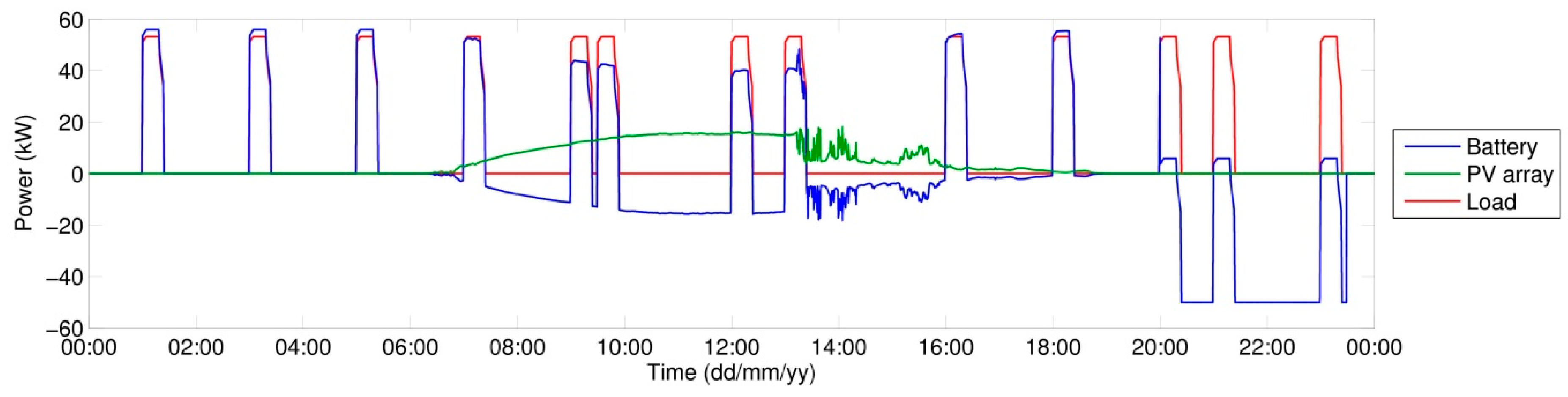
Within the operating measurement, power was measured on the DC-DC converter output (CH1—Figure 11), on the interface of battery system (CH2—Figure 11) and on the DC-AC inverter output (CH3—Figure 11). As mentioned above (part 3.5.) the profiles measured are given in Figure 10. For the power profile on battery, a negative value indicates battery charging while a positive value indicates battery discharging.
Simulation Results for the Day Measured
To check the results of assembled model, a simulation was made with input parameters measured the same day the measurement was performed of the power flows given in Figure 10.
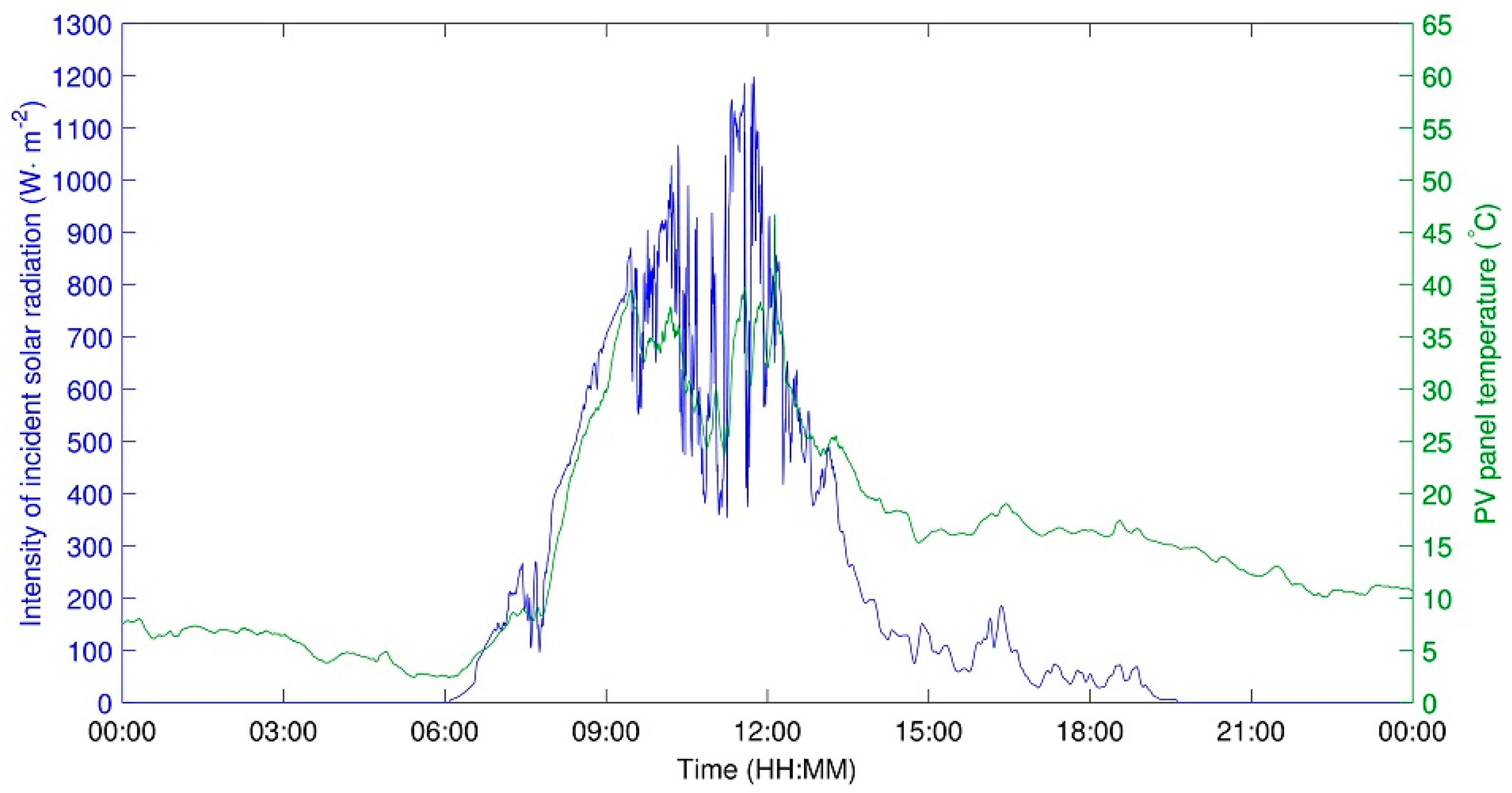
The input variables used in the simulation (module temperature, intensity of solar radiation) stem from actual measurements and their profiles are shown in Figure 12. The intensity of incident solar radiation in the panel plane was measured with a CMP21 secondary standard pyranometer, with the panel temperature being measured with a PT100 resistance temperature sensor on the rear side of the panel. The values measured describe the time profile of the quantities on 15 April 2016.
The resulting profiles for individual quantities that constitute the simulation output are given together with the resulting energy amounts given in Figure 13 and Table 2, Table 3 and Table 4.
As is obvious from the results given above, the assembled model exhibits for energy fed into accumulation a 15% deviation (ΔE_battplus—Table 4), which is primarily due to the choice of a different method of charging the lead-acid battery, where the function of three-stage charging (bulk stage, absorption stage, float stage) is not implemented in the model as is usually the case with lead-acid accumulators [21] but, for simplicity, the one-stage charging system was chosen. It can be assumed, however, that in the case of using a Li-Ion accumulator the three-stage charging will not be applied and the model error will be smaller. For simulating the scenarios of the proposed concept of employing a supporting storage system for fast charging stations for EVs, the model accuracy is sufficient in the context of the employed measurement facility (Hioki) and thus the designed model can be utilized in the simulation of individual scenarios and of the effect of the setting of individual parameters on the results (e.g., changes in the size of PVS, changes in the battery size).
5. Simulation of Results of Concept of Supporting Storage System for Fast Charging Stations for EVs
To enable implementing the simulation of an electric circuit or a device represented by means of special block from the Simscape Power Systems library, it is necessary to insert the Powergui block into the model. It is used to save the equivalent Simulink circuit which represents a set of inputs, outputs and state variables (state space) [22]. Relations between them are described by differential equations. The Powergui block offers choosing from several integration methods for solving and simulating electric circuits and devices in the designed model, specifically the continuous, discrete and phasor methods of solution [23]. When simulating dynamic systems, the solution proceeds by successive steps (time intervals in which the calculation of individual states of the system takes place) until the total simulation time is reached [24]. The simulation step can be of fixed or variable length of time.
The continuous integration method employs for simulation an integration algorithm with variable step. Its advantage consists in its greater accuracy when simulating small systems with a small number of non-linear elements and also in the shorter time necessary for the simulation of model results because the number of steps necessary for the solution is lower. A disadvantage is that the speed of simulating extensive systems containing a great number of non-linear elements decreases rapidly due to the inaccuracy of the method. In the case of simulating large systems containing more than 50 electric states of more than 25 electronic devices it is of advantage to use the discrete integration method with fixed step [22]. This method is primarily designed for strictly discrete models and it calculates their state in the nearest time step. The phasor method of solution is advantageous in cases when it is necessary to know just the magnitude and phase of voltages and currents (e.g., when solving problems related to electric grid stability), i.e., in cases when it is not necessary to solve a complete set of differential equations and the state space is substituted with the so-called reduced state space, which results in greatly increased calculation speed.
In order to simulate the behavior of the proposed system of supporting storage system for fast charging stations for EVs, it was necessary to simulate/determine the load diagram of a one station during charging an electric vehicle. Based on performed analysis and the data provided by the distribution system operator, the diagram shown in Figure 14 is considered. This AC network load diagram represents one electric vehicle charging with a 50 kW fast-charging station (FChS). The charging cycle lasts 30 min, including a 5 min service interval in the end of the cycle. The charging cycle corresponds to the charging of the one EV with a total capacity of 25 kWh. The presented cycle considers the charging from 0% SOCEV to 80% SOCEV of the one EV’s capacity.
The technical solutions that can be used for the proposed concept are currently being implemented by ABB (Energy Storage System), Schneider Electric (Energy Storage System), Siemens (Siestorage), but the usable area is generally aimed on supporting network services and improving the quality of electricity. The specific technical solution in cooperation with the fast-charging station for EVs and the PV system is not known to the authors.
5.1. Operating Scenario A—Description and Assessment
The simulated scenario employs meteorological data for the first week of September 2016. The load diagram represents a charging cycle of 13 EVs in the course of each day (the same for each day) using one 50 kW fast charging station. The charging of an EV with an accumulator capacity of 25 kWh is considered, with each EV-charging cycle considered in the 0–80% SOCEV range of the EV accumulator. One charging cycle thus represents ca 20 kWh of electric energy and takes about half an hour [10].
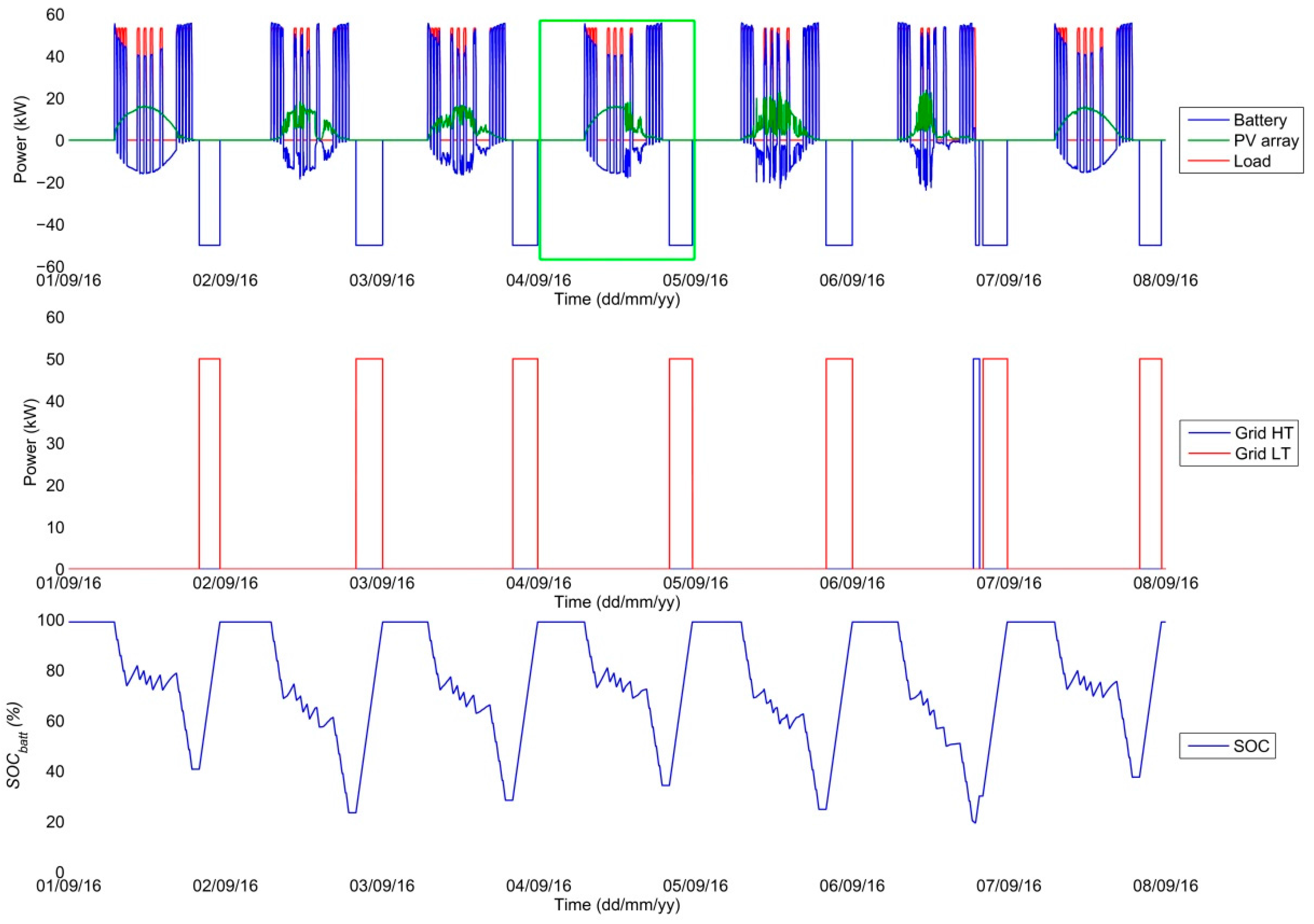
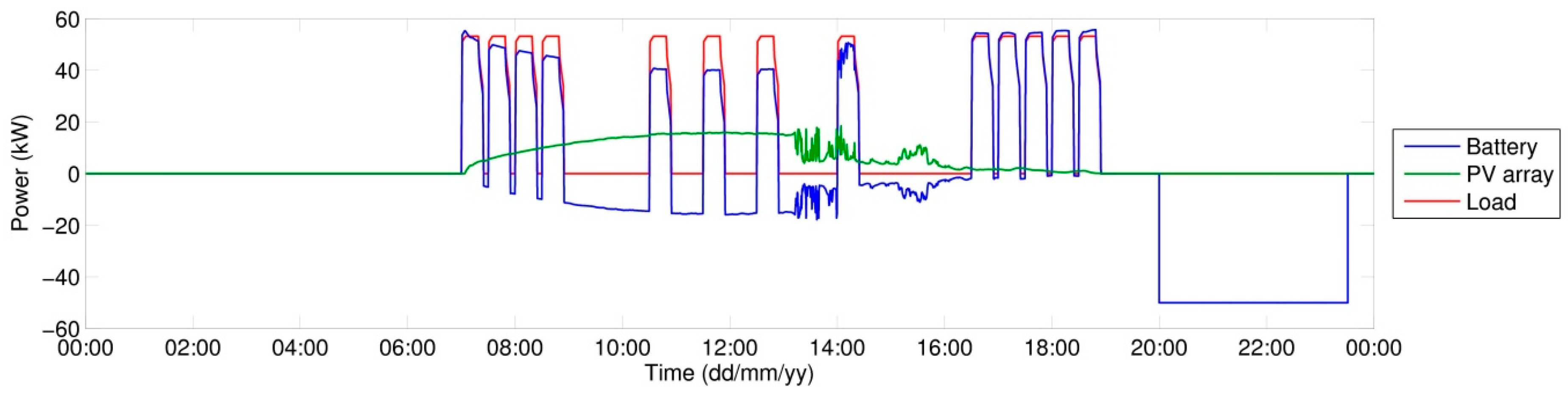
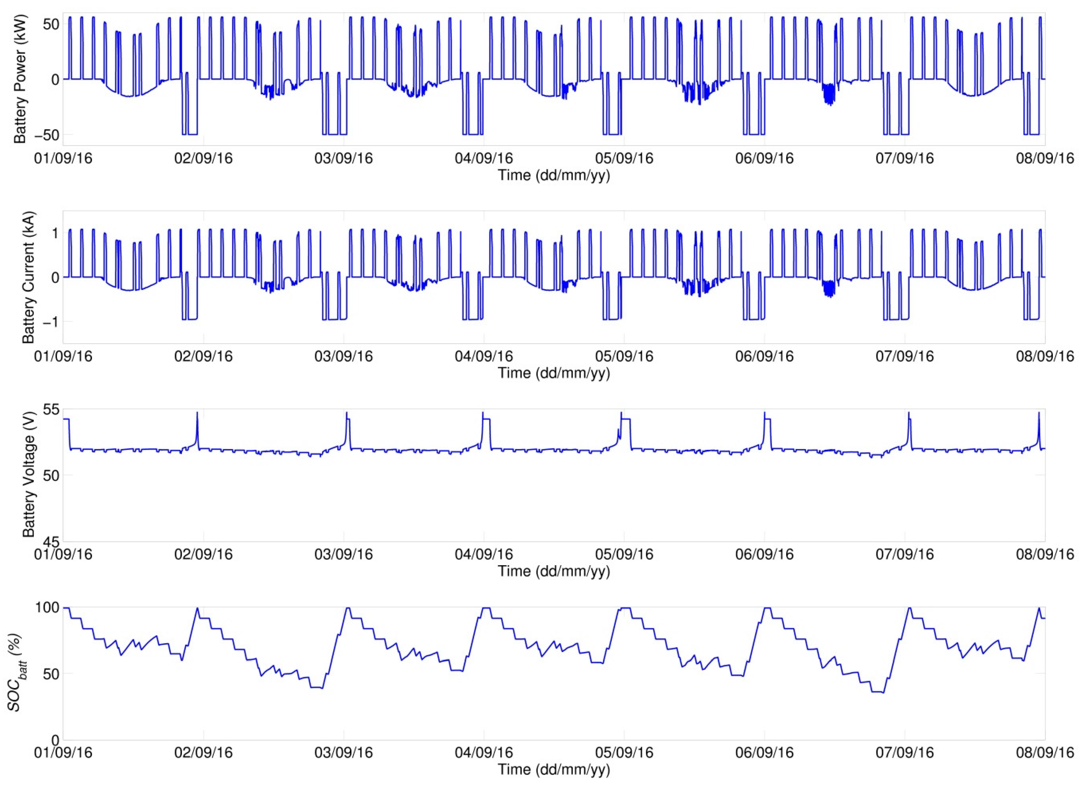
Graphical outputs from the simulation of scenario A are given in Figure 15, Figure 16 and Figure 17. Figure 18 gives a detailed view of the green-marked region in the week survey (Figure 15), specifically the 4th day of simulation. The operation of the EV-charging station considered is only in the period from 7 a.m. to 7 p.m. and this is reflected in the time distribution of EV-charging cycles, which is, moreover, concentrated into the morning and evening peaks (red curve in Figure 18).
The chosen maximum power drawn from the grid was 50 kW (this value is derived from the 3 × 80 A protection element used—prescribed protection for operating one fast charging station). If a LT period of 8 h per day is considered—this mode is valid for the duration of LT (8 h during time periods between 6 p.m. and 8 a.m.), then up to 400 kWh can theoretically be drawn from the grid during the LT period. This value represents the maximum capacity of supporting storage that is worth considering from the economic point of view.
The voltage considered for the Li-Ion storage is 48 V, capacity 5208 Ah (250,000 Wh/48 V), which represents a nominal capacity of ca 250 kWh. For the beginning of simulation the fully charged supporting accumulator is considered.
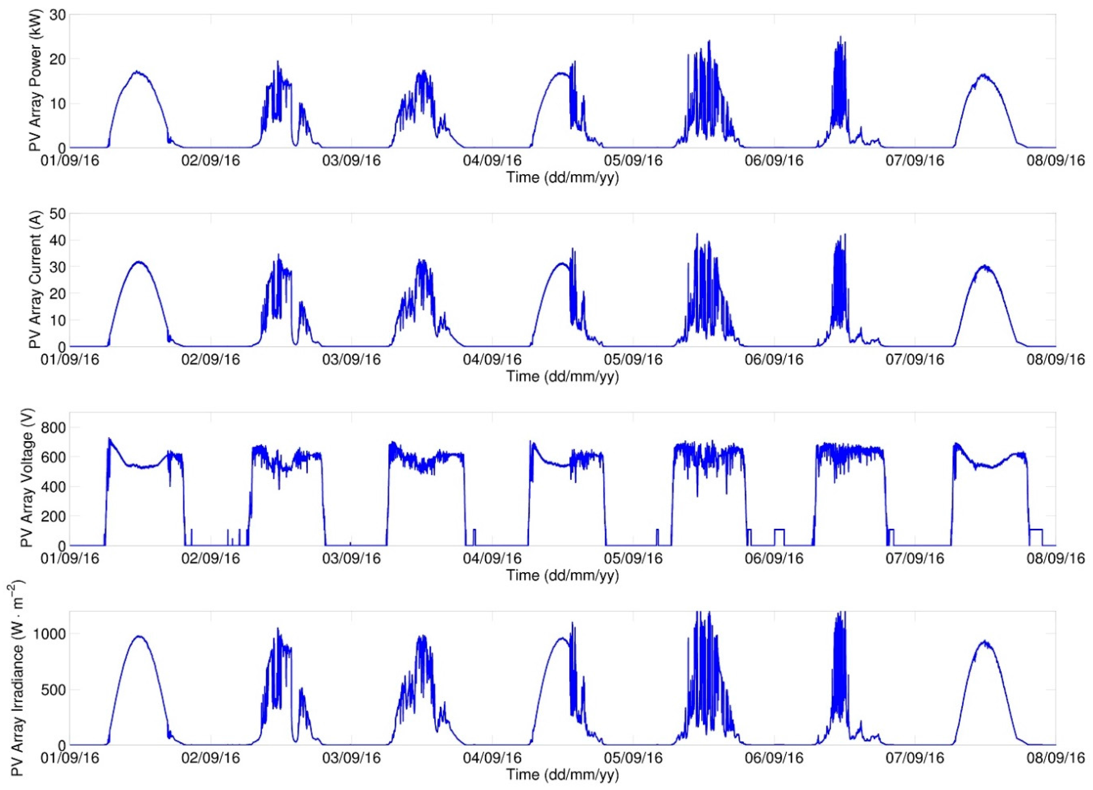
The PVS is formed by 4 parallel-interconnected strings, each made up of 20 panels, 250 Wp power each. These are PV panels of the same parameters as those used in the model validation (Table 1). The total power of the installed PV panels is thus 20 kWp.
In view of the priority to maintain the operability of fast charging station, the grid charging of the system is considered such that with the SOCbatt of the support accumulator decreasing to 20%, the charging should start irrespective of the low/high tariff. As is obvious from the algorithm of internal logic given in Figure 9, if grid charging takes place in the HT period, the charging is terminated when 30% SOCbatt is reached and the full charging of the system is preferentially performed in the LT period. For every day, the considered LT period in simulation is from 8 p.m. to 4 a.m., in keeping with the valid regulations of the operator of the electricity grid of CR.
As is obvious from the profiles given above, the chosen capacity of supporting storage (250 kWh) is sufficient for the operation of charging station, with the charging performed preferentially in LT periods. The 6th simulation day is an exception, when due to the drop of SOCbatt to the stipulated level it was necessary to start charging even in the HT period (Figure 15). As expected, HT charging was terminated when 30% SOCbatt was reached. Thus the indispensable reserve is provided for completing the charging cycle of EVs in case the station is unexpectedly disconnected from the grid. The minimum 20% SOCbatt was chosen with a view to accumulator lifetime and also as a reserve for supplying the system’s own consumption.
The plotted profiles of simulated quantities correspond with anticipated results. In Figure 17, an increase in PV Array Voltage during night hours can be seen, which relates directly to the input data of the measured intensity of solar radiation. In data sets there appears the value (2·W·m−2) for night hours, which may be due to a measurement error but it is probably the effect of ambient illumination and moonlight. The model thus responds to input values while MPPT tries to set the value of operating voltage. But because of insufficient irradiation, no current is generated and the power of PV field remains zero.
Overall energy balances of the simulated scenario are given in Table 5. As can be seen, the total energy drawn from the grid (E_GRID) amounts to 1333 kWh, from which amount 1289 kWh, i.e., 96.7%, were drawn in the LT period (E_GRID_LT), which from operation viewpoint represents an economic benefit.
5.2. Operating Scenario B—Description and Assessment
The simulated scenario B differs from scenario A in the load diagram; there are again 13 EVs under consideration but the time distribution of individual EV arrivals is different, spread over the whole day. The other simulation parameters remained the same, with a view to the possibility of a direct comparison of results. The simulation results for scenario B are shown in Figure 19, Figure 20 and Figure 21. The different distribution of EVs (red curve) in the course of the day compared to scenario A can be seen in Figure 22. As can be seen from the results given, SOCbatt does not drop to the 20% level and HT charging is not applied. The different load diagram thus has a direct impact on the ratio of energy amount E_GRID_LT to E_GRID. From the viewpoint of reduced SOCbatt, a more uniformly distributed load diagram is more favourable.
The results presented confirm the assumption that with the load diagram uniformly distributed, the supporting storage system represents a limited contribution because part of the system capacity is not used. Scenario B results thus satisfy the assumptions. Energy balance results are given in Table 6.
6. Evaluation—Advantages and Disadvantages of Proposed Concept
The proposed concept of a HS with storage that serves as support for charging electric vehicles was prepared as part of current research in the area of storage systems with support from RESs. Based on the measurement performed on the experimental HS at FEEC BUT, a simulation model was assembled with optional parameters which was subsequently modified to fit the requirements of the simulation of scenarios of the proposed concept. Presented model allows simulating longer time range (month, year) with different input parameters. The calculation time of the simulation depends directly on the length of the simulated time period and the computational power of the computer.
Calculation of a detailed simulation of one week takes approximately 7 min with average personal computer. Matlab Simulink is a robust tool for data calculation and processing and therefore was chosen as a simulation tool even though there are similar simulation tools (HOMER) that can also provide the basic energy balance of the system. The assembled model needs to be further improved especially in DC-AC converter and EVs chargers. This task is the aim of follow-up research in the field of energy systems realized at the Department of Electrical Power Engineering, at the Brno University of Technology.
In connection with the integration of charging stations into the electricity grid, an increased interest is expected in facilities that can limit the reverse effects on the grid. The proposed concept of a charging station with supporting storage can in dependence on the specific locality reduce the negative reverse effects on the grid (voltage fluctuations, asymmetry, voltage magnitude). Analysis of voltage changes during FChS operation has been realized, but is beyond the aim of this paper. An optimally designed storage system (ensuring minimum HT drawing from the grid) stabilizes drawing from the grid with respect to accumulation cycling, and this has a positive effect on grid stability and, consequently, also a positive effect on the planning of electricity grid. The capacity of the accumulation system cannot be designed only with the emphasis on the maximum capacity. It is necessary to consider the number of charging/discharging cycles and the discharging rate with respect to the required technological reserve. Other aspects that define the size of accumulation are the size of system’s circuit breaker in combination with the LT duration so that the system is ready for the next working cycle.
The main economic contribution of the proposed concept can be seen in reduced operating costs due to minimum HT power drawn from the grid (difference between HT and LT electricity price), with PVS reducing still further the required amount of energy drawn from the grid (in HT periods, in particular).
The main disadvantage is the purchase price of supporting storage and converters. Based on the analyses conducted up to now, a price ranging between Euro 200,000 and 250,000 can be expected for a system with one 50 kW fast charging station, hybrid converter, LiFePO-based supporting storage of 250 kWh capacity and 20 kWp PVS.
As documented by the simulation results obtained and by data from physical measurement, the designed model can be used to simulate scenarios with different parameters and thus test the chosen configuration of individual parameters of the concept presented. Following up on the current cooperation with and requirements of the industry (the CEZ (Prague, Czech Republic) and the E.ON (České Budějovice, Czech Republic) companies) it is expected that research will further continue in areas related to the application of storage systems with the aim of limiting potential effects on the electricity grid.
Acknowledgments
Paper was prepared at Centre for Research and Utilization of Renewable Energy. Authors gratefully acknowledge financial support from the Technology Agency of the Czech Republic (project No. TH02020435) and National Feasibility Program I of Ministry of Education, Youth and Sport of the Czech Republic under project No. LO1210.
Author Contributions
Petr Mastny and Jan Moravek conceived and designed the concept of charging site. Jan Moravek and Martin Vojtek performed the measurements, data analysis and created the simulation model. Jiri Drapela consulted the results of the analysis. All of the authors have been involved in writing the manuscript.
Conflicts of Interest
The authors declare no conflict of interest.
Nomenclature
| A | diode ideality factor (-), |
| E_AC_LOAD,meas | measured value of energy drawn by load on AC side of inverter (Wh), |
| E_AC_LOAD,sim | simulation result of energy drawn by load on AC side of inverter (Wh), |
| E_battminus,meas | measured value of energy drawn from battery (Wh), |
| E_battminus,sim | simulation result of energy drawn from battery (Wh), |
| E_battplus,meas | measured value of energy fed into battery (Wh), |
| E_battplus,sim | simulation result of energy fed into battery (Wh), |
| E_DC_DC,meas | measured value of energy fed into system by DC-DC converter (Wh), |
| E_DC_DC,sim | simulation result of energy fed into system by DC-DC converter (Wh), |
| E_GRID | total amount of electric energy drawn from the grid (Wh), |
| E_GRID_HT | amount of electric energy drawn in the high-tariff (Wh), |
| E_GRID_LT | amount of electric energy drawn in the low-tariff (Wh), |
| E_PV | energy potential of PV system (Wh), |
| G | intensity of solar radiation (W·m−2), |
| Impp | maximum power point current of PV panel at STC (A), |
| Iph | current generated by photodiode (A), |
| Ipv | input current of PV panel (A), |
| Is | saturation current (A), |
| Isc | short circuit current of PV panel at STC (A), |
| Ns | number of panel cells in series (-), |
| Pbatt | power on accumulator interface (W), |
| Pgrid | power drawn from grid—max. limit (W), |
| Pgrid, HT | power drawn from grid in high-tariff periods (W), |
| Pgrid, LT | power drawn from grid in low-tariff periods (W), |
| Pin,DC-DC | DC-DC converter input power (W), |
| Pload,AC | DC-AC inverter output power (W), |
| Pload,DC | DC-AC inverter input power (W), |
| Pout,DC-DC | DC-DC converter output power (W), |
| Pout,PV | PV field output power (W), |
| Q | control coefficient (-), |
| Rs | series resistance of PV panel (Ω), |
| Rsh | shunt resistance of PV panel (Ω), |
| SOCbatt | system’s battery state of charge (%), |
| SOCEV | electric vehicle’s battery state of charge (%), |
| T | PV cell temperature (K), |
| V | output voltage of PV panel (V), |
| Vmpp | maximum power point voltage of PV panel at STC (V), |
| Voc | open circuit voltage of PV panel at STC (V), |
| Vref | reference voltage determined by the MPPT (V), |
| XL | deviation of results obtained using Lambert W function (A), |
| XNR | deviation of results obtained using Newton-Raphson method (A), |
| k | Boltzmann constant (k = 1.38 × 10⁻²³ J·K−1), |
| t | PV panel temperature (°C), |
| q | electron charge (q = 1.602 × 10⁻⁹ C), |
| ΔE_battminus | difference of energy drawn from battery (%), |
| ΔE_battplus | difference of energy fed into battery (%) |
| ΔE_AC_LOAD | difference of energy drawn by load on AC side of inverter (%), |
| ΔE_DC_DC | difference of energy fed into system by DC-DC converter (%), |
| α | short circuit current temperature coefficient (A·K−1), |
| ηDC-DC | DC-DC converter efficiency (%), |
| ηDC-AC | DC-AC inverter efficiency (%). |
References
- Czech Energy Regulatory Office. Decree No 16/2016: Conditions for Connection to the Public Electricity Grid in Czech Language; Czech Energy Regulatory Office: Jihlava, Czech Republic, 2016. [Google Scholar]
- New Green Savings Programme—Directive No. 1 NZU 2014 and Its Annexes. Czech Republic, 2014. Available online: http://www.novazelenausporam.cz/en/ (accessed on 12 December 2016). (In Czech).
- Richardson, D.B. Electric vehicles and the electric grid: A review of modeling approaches, Impacts, and renewable energy integration. Renew. Sustain. Energy Rev. 2013, 19, 247–254. [Google Scholar] [CrossRef]
- Darabi, Z.; Ferdowsi, M. Aggregated Impact of Plug-in Hybrid Electric Vehicles on Electricity Demand Profile. IEEE Trans. Sustain. Energy 2011, 2, 501–508. [Google Scholar] [CrossRef]
- Automotive Industry Association (AIA). Czech Vehicle Parc—November 2015. Available online: http://www.autosap.cz/zakladni-prehledy-a-udaje/slozeni-vozoveho-parku-v-cr/ (accessed on 18 November 2016). (In Czech).
- IEC 61815-1:2017. Electric Vehicle Conductive Charging System—Part 1: General Requirements; IEC: Geneva, Switzerland, 2017. [Google Scholar]
- Nema, P.; Nema, R.K.; Rangnekar, S. A current and future state of art development of hybrid energy system using wind and PV-solar: A review. Renew. Sustain. Energy Rev. 2009, 13, 2096–2103. [Google Scholar] [CrossRef]
- Henninger, S.; Jaeger, J.; Rubenbauer, H. Dimensioning and control of energy storage systems for renewable power leveling. In Proceedings of the 2016 IEEE/PES Transmission and Distribution Conference and Exposition (T&D), Dallas, TX, USA, 2016; pp. 1–5. [Google Scholar] [CrossRef]
- Yunus, K.; De La Parra, H.Z.; Reza, M. Distribution grid impact of Plug-In Electric Vehicles charging at fast charging stations using stochastic charging model. In Proceedings of the 2011 14th European Conference on Power Electronics and Applications, Birmingham, UK, 2011; pp. 1–11. [Google Scholar]
- Mastny, P.; Moravek, J.; Vrana, M. Concept of Fast Charging Stations with Integrated Accumulators—Assessment of the Impact for Operation. In Proceedings of the 2016 17th International Scientific Conference on Electric Power Engineering (EPE), Prague, Czech Republic, 16–18 May 2016; pp. 194–199, ISBN 978-1-5090-0907-7. [Google Scholar]
- Cubas, J.; Pindado, S.; de Manuel, C. Explicit Expressions for Solar Panel Equivalent Circuit Parameters Based on Analytical Formulation and the Lambert W-Function. Energies 2014, 7, 4098–4115. [Google Scholar] [CrossRef]
- Chan, D.S.H.; Phang, J.C.H. Analytical methods for the extraction of solar-cell single- and double-diode model parameters from I-V characteristics. IEEE Trans. Electron. Devices 1987, 34, 286–293. [Google Scholar] [CrossRef]
- Sera, D.; Teodorescu, R.; Rodriguez, P. PV panel model based on datasheet values. In Proceedings of the 2007 IEEE International Symposium on Industrial Electronics, Vigo, Spain, 2007; pp. 2392–2396. [Google Scholar] [CrossRef]
- Orioli, A.; Di Gangi, A. A procedure to calculate the five-parameter model of crystalline silicon photovoltaic modules on the basis of the tabular performance data. Appl. Energy 2013, 102, 1160–1177. [Google Scholar] [CrossRef]
- Siddique, H.A.B.; Xu, P.; De Doncker, R.W. Parameter extraction algorithm for one-diode model of PV panels based on datasheet values. In Proceedings of the 2013 International Conference on Clean Electrical Power (ICCEP), Alghero, Italy, 2013; pp. 7–13. [Google Scholar] [CrossRef]
- De Brito, M.A.G.; Sampaio, L.P.; Luigi, G., Jr.; e Melo, G.A.; Canesin, C.A. Comparative Analysis of MPPT Techniques for PV Applications. In Proceedings of the 2011 International Conference on Clean Electrical Power (ICCEP), Ischia, Italy, 14–16 June 2011. [Google Scholar]
- Piegari, L.; Rizzo, R.; Spina, I.; Tricoli, P. Optimized Adaptive Perturb and Observe Maximum Power Point Tracking Control for Photovoltaic Generation. Energies 2015, 8, 3418–3436. [Google Scholar] [CrossRef]
- Batunlu, C.; Alrweq, M.; Albarbar, A. Effects of Power Tracking Algorithms on Lifetime of Power Electronic Devices Used in Solar Systems. Energies 2016, 9, 884. [Google Scholar] [CrossRef]
- Femia, N.; Petrone, G.; Spagnuolo, G.; Vitelli, M. Optimization of perturb and observe maximum power point tracking method. IEEE Trans. Power Electron. 2005, 20, 963–973. [Google Scholar] [CrossRef]
- Moravek, J.; Mastny, P. Hybrid renewable energy system—Configuration and control. Recent Res. Electr. Power Energy 2013, 22, 87–92. [Google Scholar]
- Wu, Y.; Shen, C.; Liu, C. Implementation of solar illumination system with three-stage charging and dimming control function. In Proceedings of the 2011 International Conference on Electric Information and Control Engineering, Wuhan, China, 15–17 April 2011; pp. 2260–2263. [Google Scholar] [CrossRef]
- The MathWorks, Inc. Available online: http://www.mathworks.com/help/physmod/sps/powersys/ref/powergui.html?searchHighlight=powergui (accessed on 16 December 2016).
- The MathWorks, Inc. Available online: http://www.mathworks.com/help/physmod/sps/powersys/ug/choosing-an-integration-method.html (accessed on 16 December 2016).
- The MathWorks, Inc. Available online: http://www.mathworks.com/help/simulink/ug/choosing-a-solver.html (accessed on 16 December 2016).
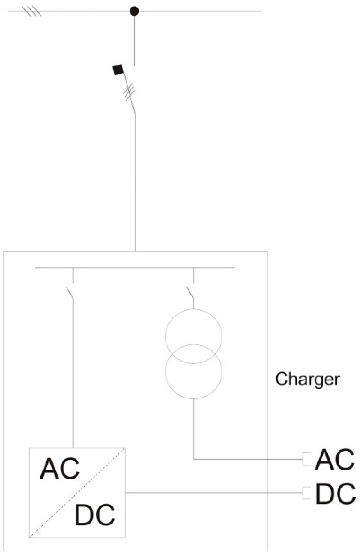
Figure 1.
General one-phase connection of charging station.

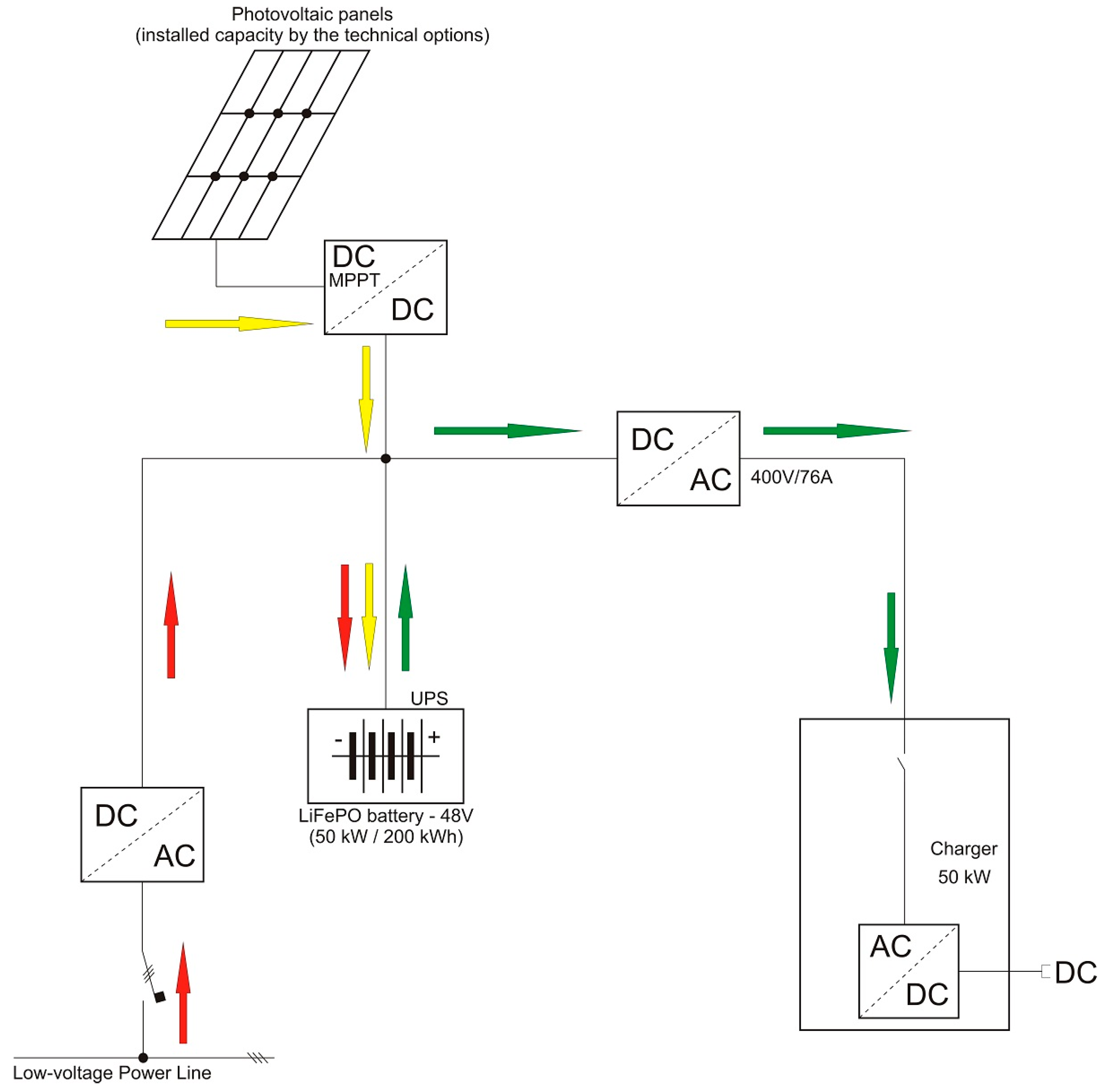
Figure 2.
Concept of a charging station with renewable energy source (RES) support and accumulation [10].
Figure 2.
Concept of a charging station with renewable energy source (RES) support and accumulation [10].

Figure 3.
Implementation of a hybrid system (HS) in the Matlab Simulink programming environment.

Figure 4.
Equivalent schematic of one-diode model of photovoltaic (PV) panel acc. to [11].
Figure 4.
Equivalent schematic of one-diode model of photovoltaic (PV) panel acc. to [11].
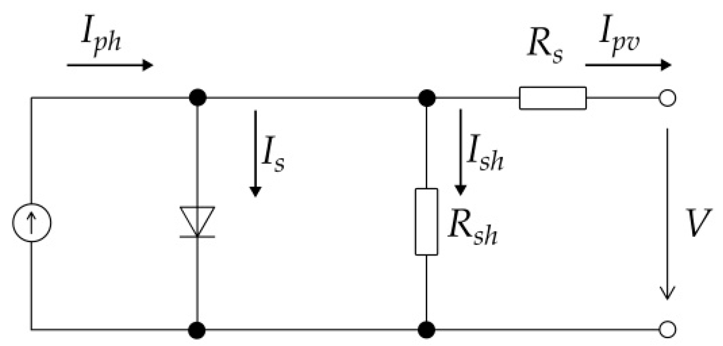
Figure 5.
Comparison of measured I-V curve and simulation results.

Figure 6.
Topology of PV field model in Matlab programming environment.

Figure 7.
Dependence of control coefficient on instantaneous battery voltage.

Figure 8.
Basic P&O algorithm, according to [16].
Figure 8.
Basic P&O algorithm, according to [16].
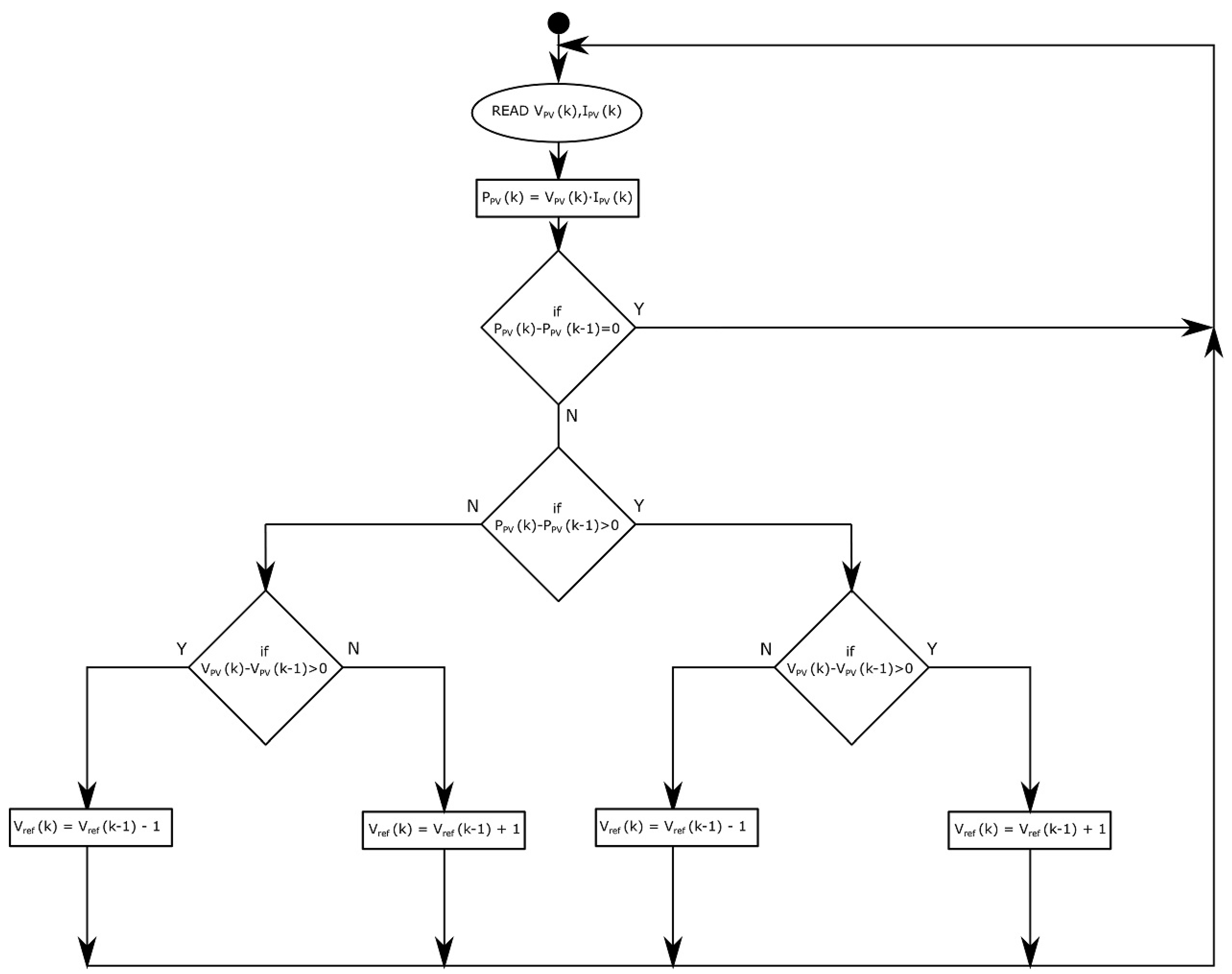
Figure 9.
Control algorithm for charging up supporting storage.
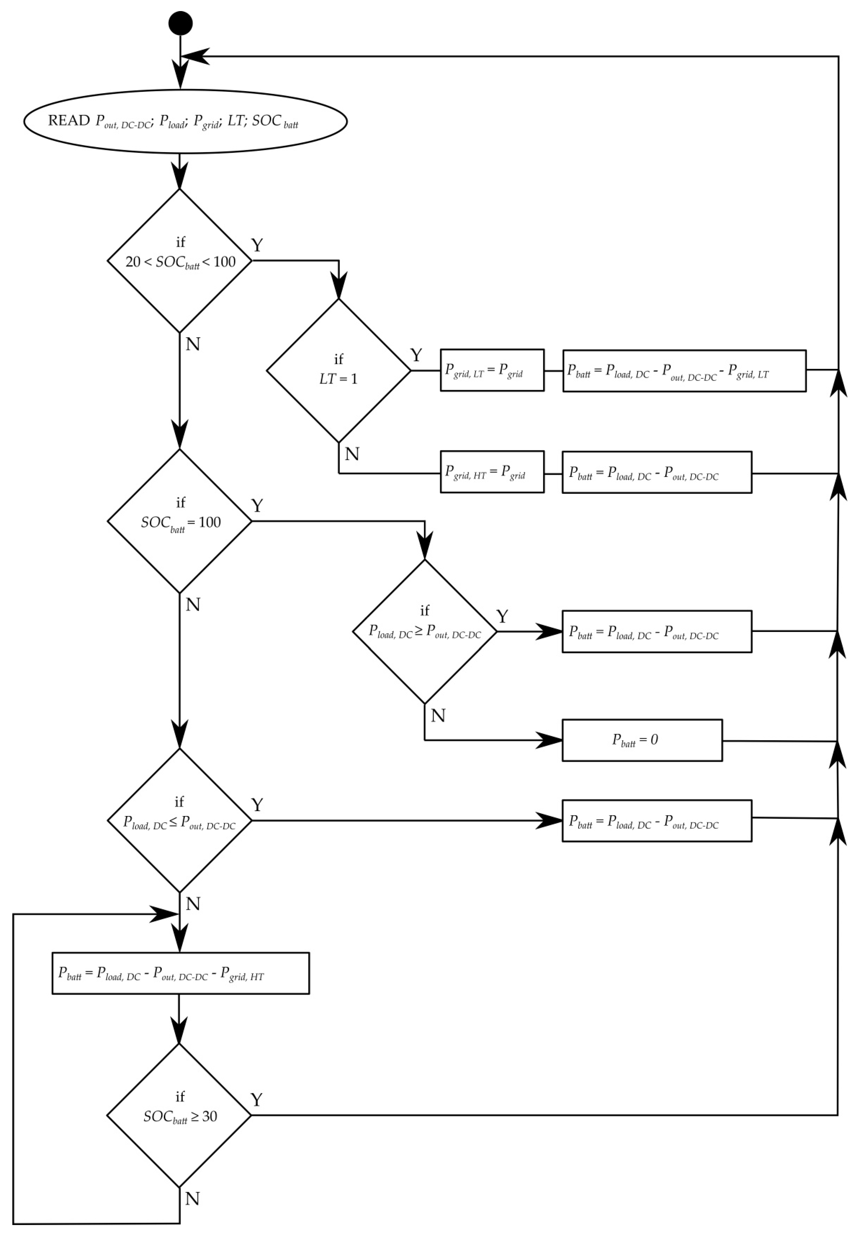
Figure 10.
Power profiles measured on physical model of HS.

Figure 11.
Schematic of experimental HS, with measuring points marked.
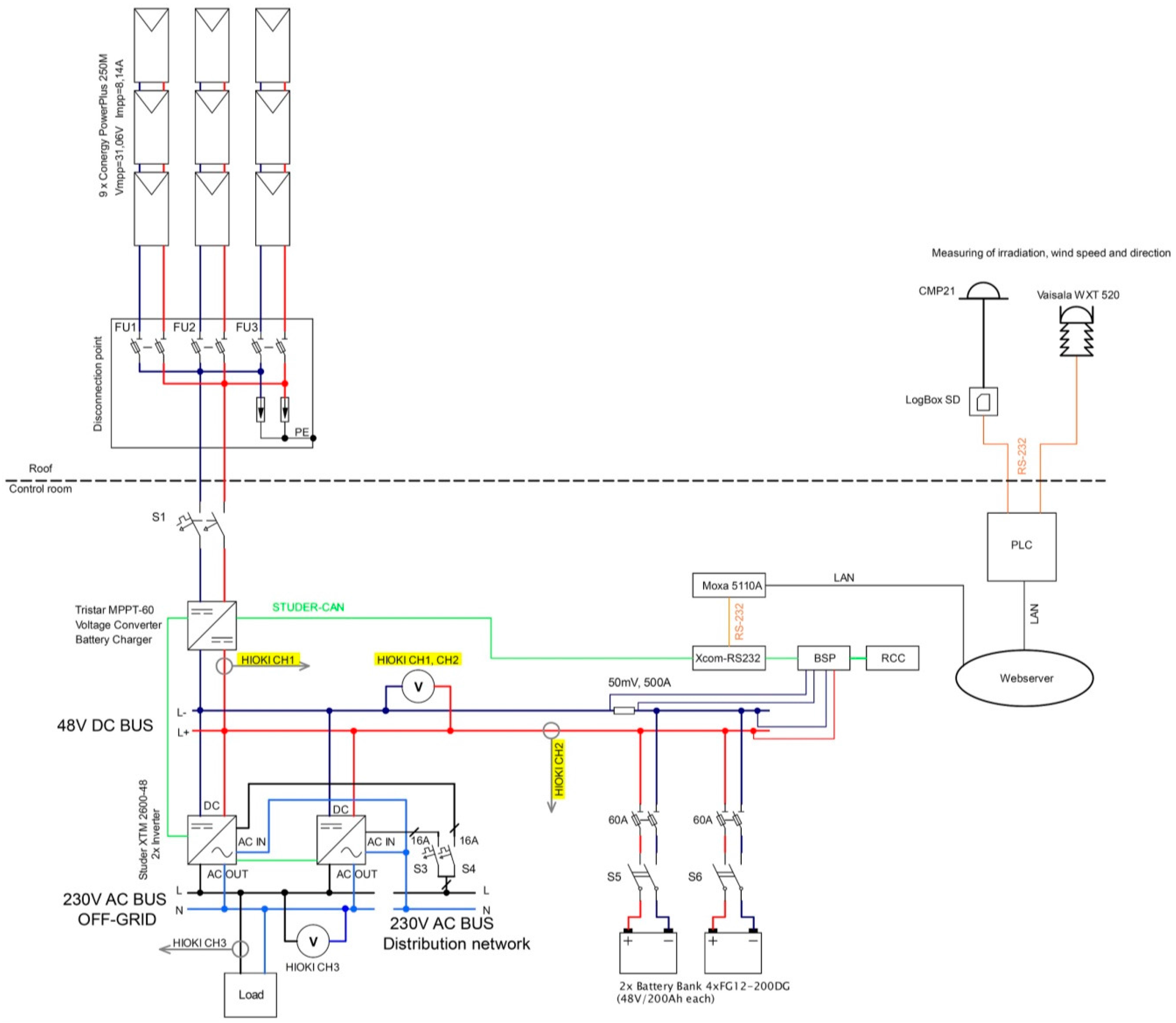
Figure 12.
Intensity vs. time profile of solar radiation incident on PV field and PV panel temperature.
Figure 12.
Intensity vs. time profile of solar radiation incident on PV field and PV panel temperature.

Figure 13.
Power vs. time profiles obtained from simulation on HS model.
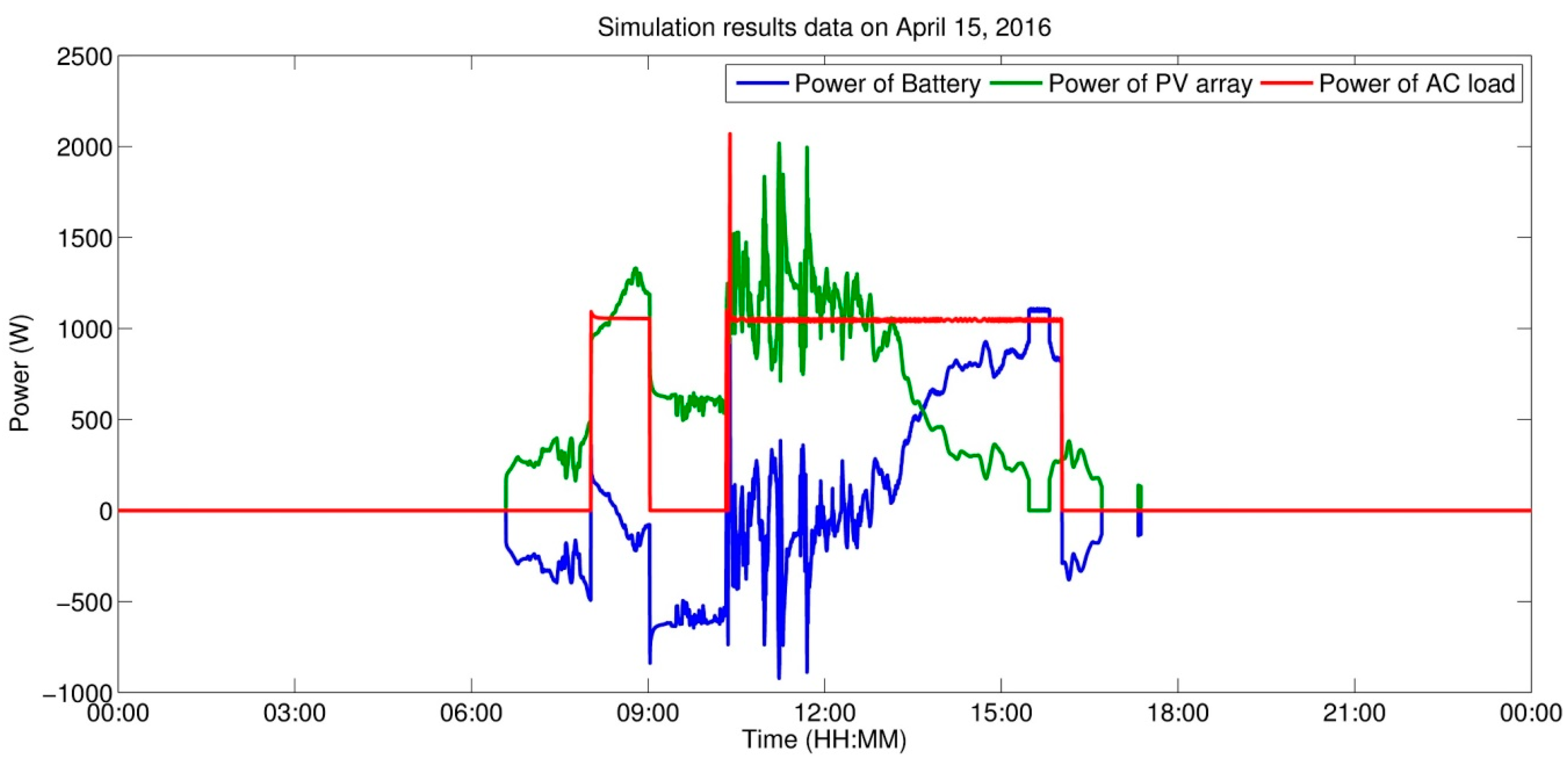
Figure 14.
Load active power vs. time for one EV charging cycle.
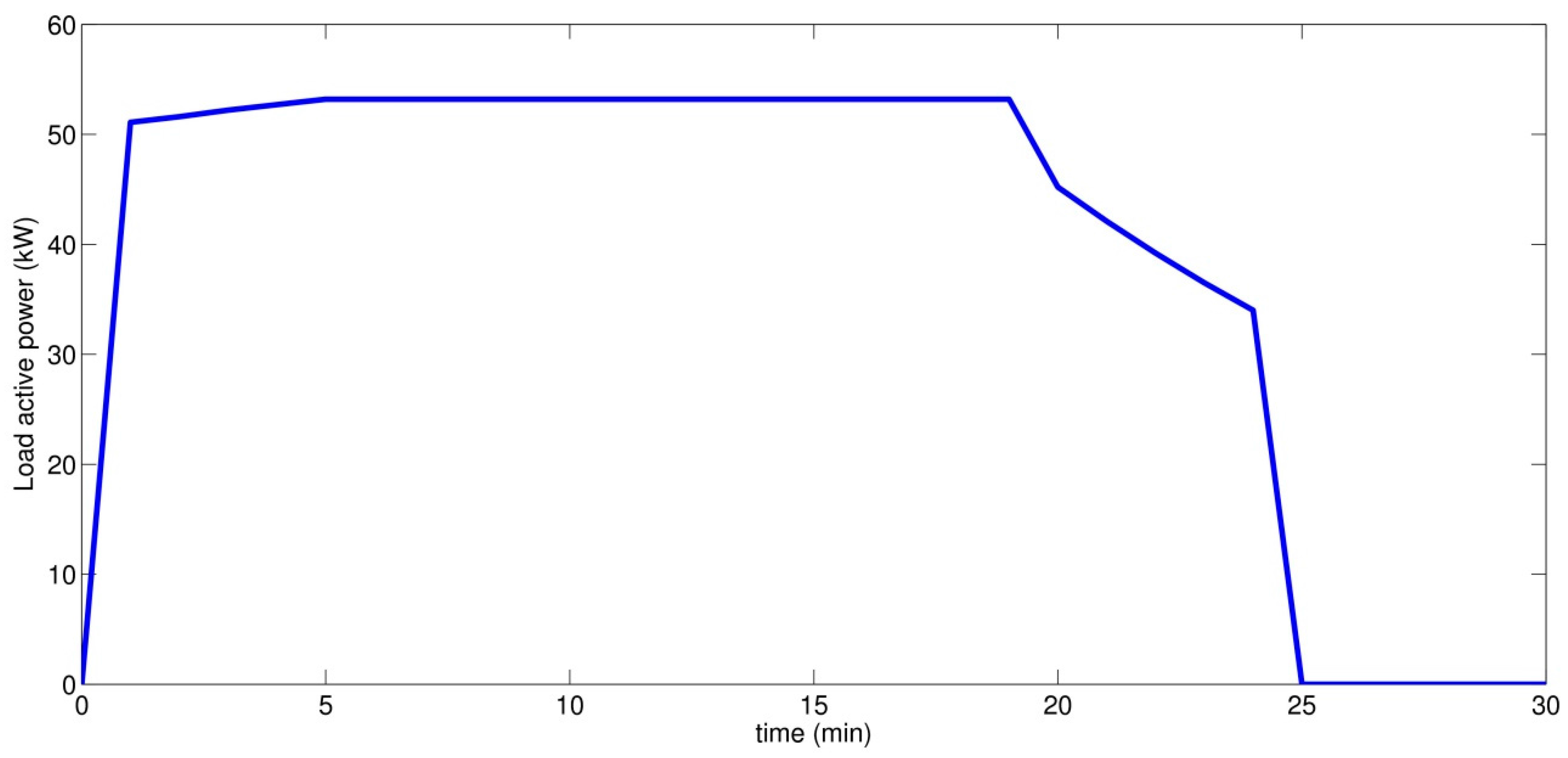
Figure 15.
Resulting profiles in simulation of individual states—overall survey, scenario A.

Figure 16.
Resulting profiles of simulation of operating states of accumulation, scenario A.
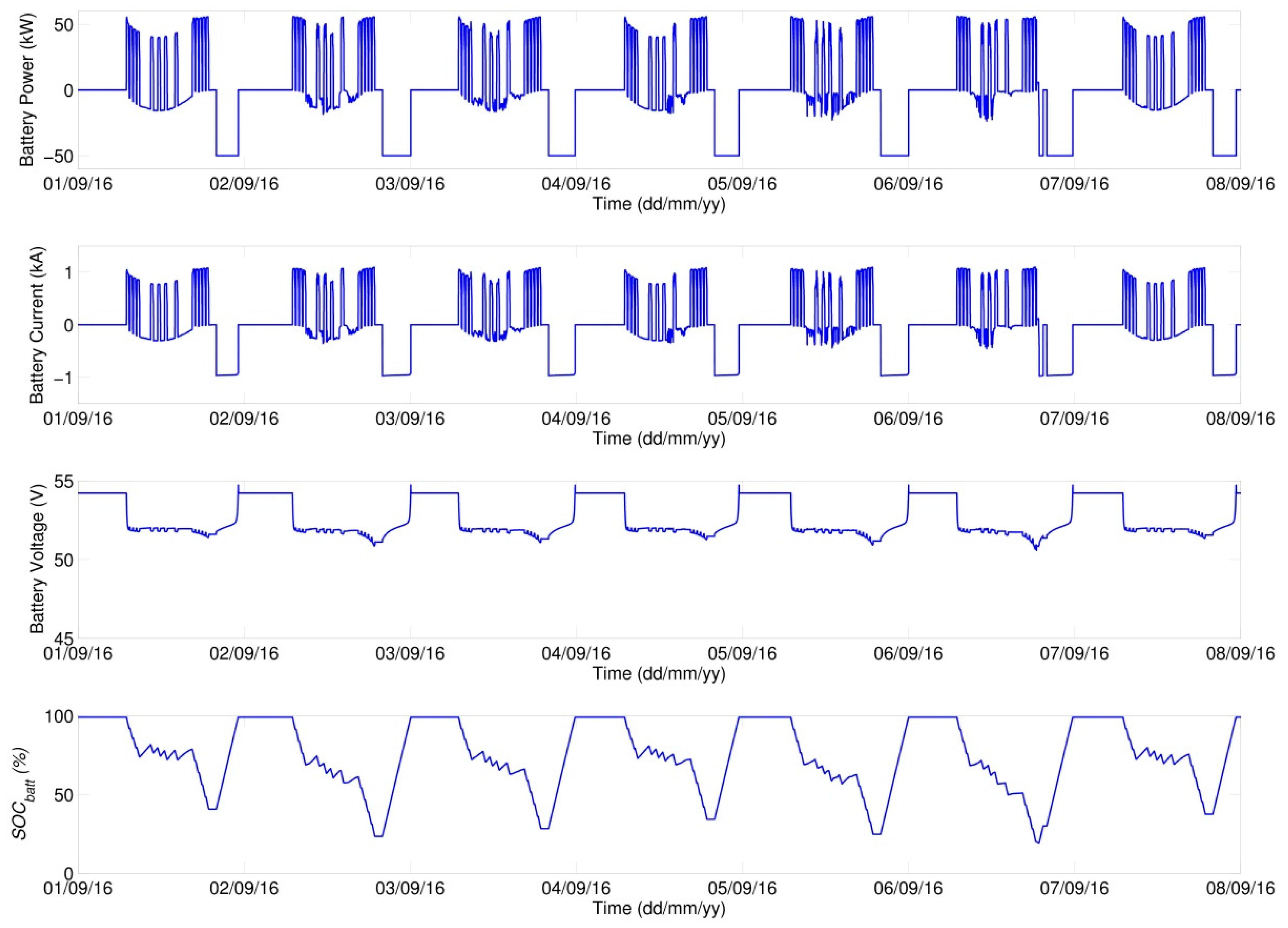
Figure 17.
Resulting profiles of simulation of operating states of photovoltaic system (PVS), scenario A.
Figure 17.
Resulting profiles of simulation of operating states of photovoltaic system (PVS), scenario A.
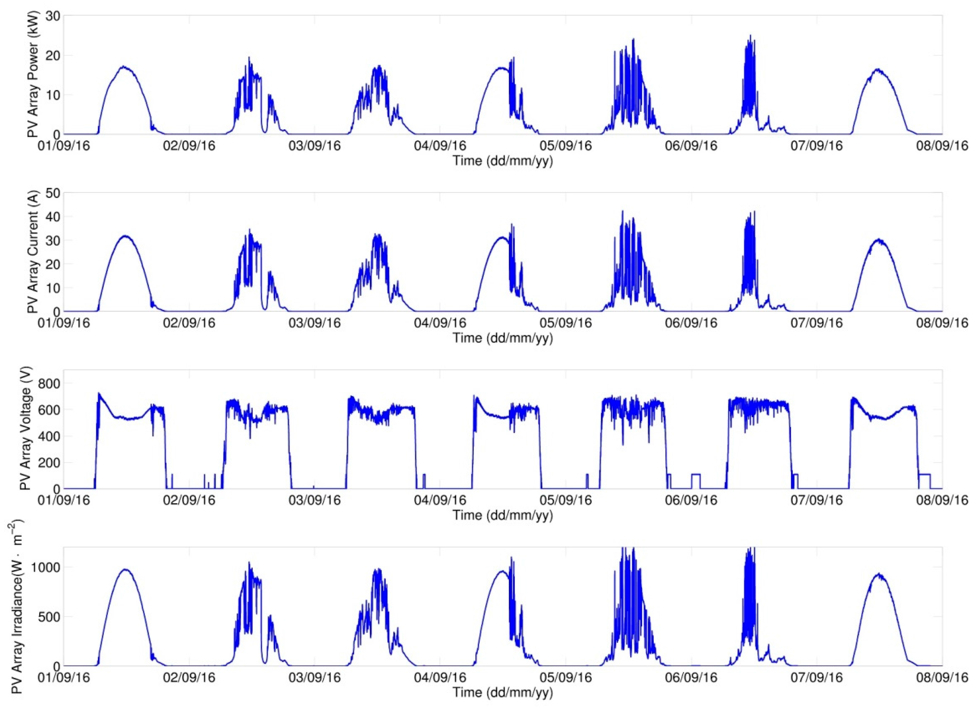
Figure 18.
Power profiles in simulation of individual states, scenario A–detailed view of 4th day.

Figure 19.
Resulting profiles for simulation of individual states—general overview, scenario B.
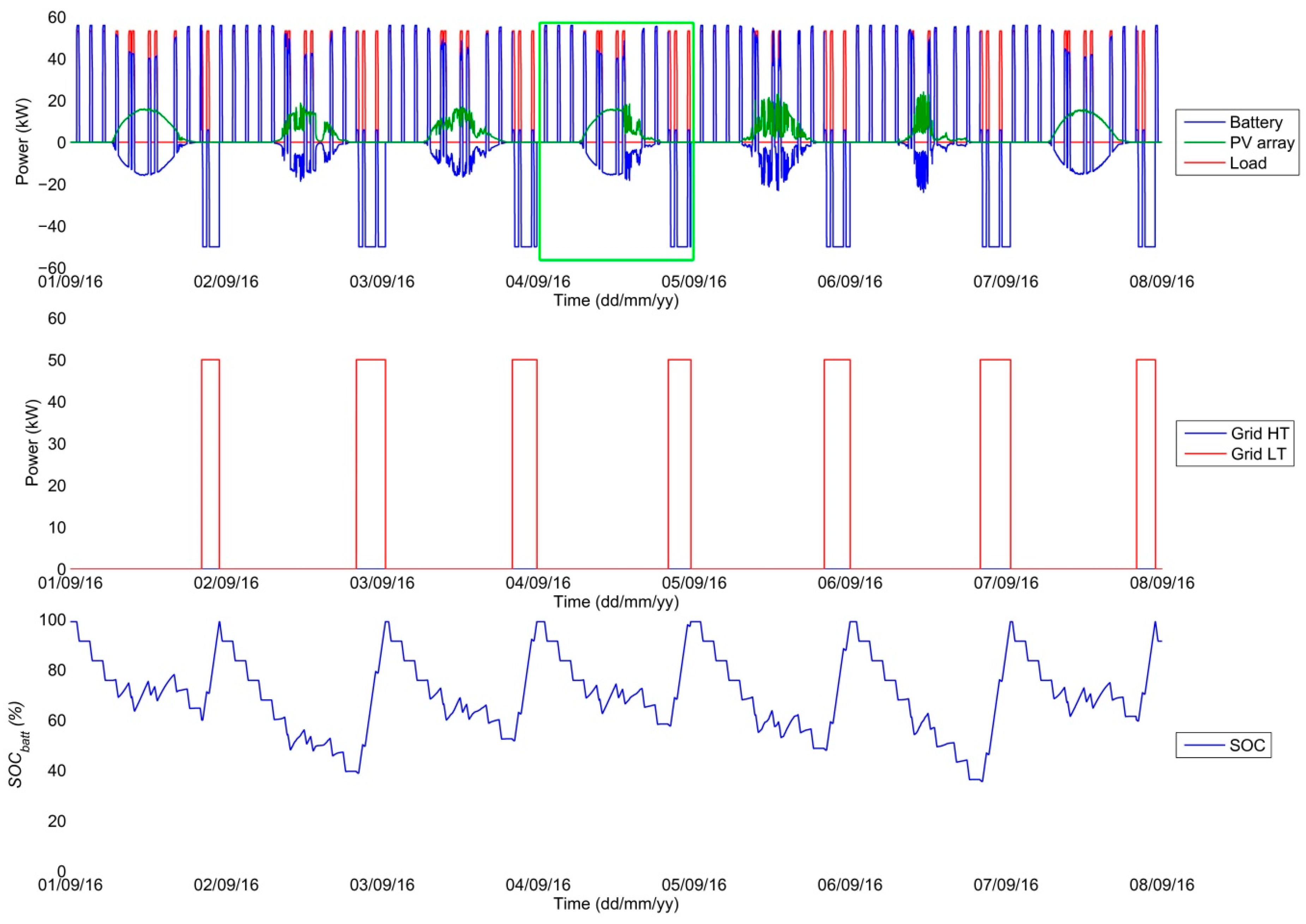
Figure 20.
Resulting profiles for simulation of operating states of accumulation, scenario B.

Figure 21.
Resulting profiles for simulation of operating states of PVS, scenario B.

Figure 22.
Power profile for simulation of individual states, scenario B, detailed view of 4th day.

Table 1.
Parameters of simulated photovoltaic (PV) panel. Standard Test Conditions (STC); MPP: maximum power point.
Table 1.
Parameters of simulated photovoltaic (PV) panel. Standard Test Conditions (STC); MPP: maximum power point.
| Parameter | Value | Note |
|---|---|---|
| Short circuit current at STC | Isc = 8.66 A | from datasheet |
| Open circuit voltage at STC | Voc = 37.9 V | from datasheet |
| MPP current at STC | Impp = 8.14 A | from datasheet |
| MPP voltage at STC | Vmpp = 31.1 V | from datasheet |
| Number of cells in series | Ns = 60 | from datasheet |
| Short circuit current temperature coefficient | α = 0.0051 A·K−1 | from datasheet |
| Ideality factor | A = 1.102 | Calculated using the Newton-Raphson iteration method |
| Series resistance | Rs = 0.277 Ω | Calculated using the Newton-Raphson iteration method |
| Shunt resistance | Rsh = 1600 Ω | Calculated using the Newton-Raphson iteration method |
| Series resistance | Rs = 0.228 Ω | Calculated using the Lambert W function |
| Shunt resistance | Rsh = 625 Ω | Calculated using the Lambert W function |
Table 2.
Energy comparison during validation—measured values.
| Name | Quantity Designation | Value |
|---|---|---|
| Energy drawn by load on AC side | E_AC_LOAD,meas | 7.021 kWh |
| Energy fed into system by DC-DC converter | E_DC_DC,meas | 6.823 kWh |
| Energy drawn from battery | E_battminus,meas | 2.333 kWh |
| Energy fed into battery | E_battplus,meas | 1.548 kWh |
Table 3.
Energy comparison during validation—simulation results.
| Name | Quantity Designation | Value |
|---|---|---|
| Energy drawn by load on AC side | E_AC_LOAD,sim | 7.021 kWh |
| Energy fed into system by DC-DC converter | E_DC_DC,sim | 6.818 kWh |
| Energy drawn from battery | E_battminus,sim | 2.361 kWh |
| Energy fed into battery | E_battplus,sim | 1.789 kWh |
Table 4.
Energy comparison during validation–percentage difference.
| Name | Quantity designation | Value |
|---|---|---|
| Energy drawn by load on AC side | ΔE_AC_LOAD | 0% |
| Energy fed into system by DC-DC converter | ΔE_DC_DC | −0.07% |
| Energy drawn from battery | ΔE_battminus | +1.2% |
| Energy fed into battery | ΔE_battplus | +15% |
Table 5.
Resulting energy balances for scenario A.
| Name | Quantity Designation | Value |
|---|---|---|
| Overall energy drawn from grid | E_GRID | 1333 kWh |
| Energy drawn from grid during LT | E_GRID_LT | 1289 kWh |
| Energy drawn by load on AC side | E_AC_LOAD | 1824 kWh |
| Energy drawn by load on DC side | E_DC_LOAD | 1915 kWh |
| Energy potential of PV system | E_PV | 630 kWh |
| Energy fed into system by DC-DC converter | E_DC_DC | 590 kWh |
| Energy fed into battery | E_battminus | 1698 kWh |
| Energy drawn from battery | E_battplus | 1687 kWh |
| Balance of stored energy | E_batt | 11 kWh |
Table 6.
Resulting energy balances for scenario B.
| Name | Quantity Designation | Value |
|---|---|---|
| Overall energy drawn from grid | E_GRID | 1303 kWh |
| Energy drawn from grid under LT | E_GRID_LT | 1303 kWh |
| Energy drawn by load on AC side | E_AC_LOAD | 1824 kWh |
| Energy drawn by load on DC side | E_DC_LOAD | 1915 kWh |
| Energy potential of PV system | E_PV | 630 kWh |
| Energy fed into system by DC-DC converter | E_DC_DC | 600 kWh |
| Energy fed into battery | E_battminus | 1408 kWh |
| Energy drawn from battery | E_battplus | 1420 kWh |
| Balance of stored energy | E_batt | −12 kWh |
© 2017 by the authors. Licensee MDPI, Basel, Switzerland. This article is an open access article distributed under the terms and conditions of the Creative Commons Attribution (CC BY) license (http://creativecommons.org/licenses/by/4.0/).
Share and Cite
MDPI and ACS Style
Mastny, P.; Moravek, J.; Vojtek, M.; Drapela, J. Hybrid Photovoltaic Systems with Accumulation—Support for Electric Vehicle Charging. Energies 2017, 10, 834. https://doi.org/10.3390/en10070834
AMA Style
Mastny P, Moravek J, Vojtek M, Drapela J. Hybrid Photovoltaic Systems with Accumulation—Support for Electric Vehicle Charging. Energies. 2017; 10(7):834. https://doi.org/10.3390/en10070834
Chicago/Turabian StyleMastny, Petr, Jan Moravek, Martin Vojtek, and Jiri Drapela. 2017. "Hybrid Photovoltaic Systems with Accumulation—Support for Electric Vehicle Charging" Energies 10, no. 7: 834. https://doi.org/10.3390/en10070834
Note that from the first issue of 2016, this journal uses article numbers instead of page numbers. See further details here.