Article

A Methodology for Determining Permissible Operating Region of Power Systems According to Conditions of Static Stability Limit

1
The University of Danang, 41 Le Duan st., Danang 59000, Vietnam
2
Department of Electrical Engineering, The University of Danang—University of Science and Technology, 54 Nguyen Luong Bang st., Danang 59000, Vietnam
3
Department of Energy, Polytechnic University of Milan, via La Masa, 34, 20156 Milan, Italy
*
Author to whom correspondence should be addressed.
Energies 2017, 10(8), 1163; https://doi.org/10.3390/en10081163
Submission received: 6 April 2017 / Revised: 13 July 2017 / Accepted: 4 August 2017 / Published: 17 August 2017
(This article belongs to the Special Issue Distributed and Renewable Power Generation)

Abstract

:
For power systems with long-distance ultra-high-voltage (UHV) transmission lines, power transmission limits are often determined by static stability limits. Therefore, the assessment of stability and finding solutions to improve the stability reserve are essential for the operation of the system. This article presents an analytical approach to construct limit characteristics according to static stability conditions on a power plane. Based on the approach proposed, a program is developed and tested on a system with long-distance UHV transmission lines, showing a good performance.

1. Introduction

The rapid development of economies, science, and technology in the world has led to an increasing demand for energy consuming in general and electricity in particular. Power systems are growing and expanding to link power systems of regions or to connect large power plants to consumers using ultra-high-voltage (UHV) or extra-high-voltage (EHV) transmission lines. Large interconnected power systems with long UHV or EHV lines have different features to small ones. The presence of a large amount of reactive power generated by a high voltage line during its operation influences the transmission capacity of the line and the stability of the system.
The definition and classification of power system stability are given in detail in [1]. Power system stability is broadly classified into three categories [1]: rotor angle stability [2,3,4], frequency stability [5,6] and voltage stability [7]. Voltage stability is defined as the ability of a system to maintain steady voltages at all buses in the system after being subjected to a disturbance from a given initial operating condition [1,7]. In voltage stability analysis, it is useful to further classify voltage stability into two subcategories, i.e., large disturbance and small disturbance voltage stability. The former refers to the ability of the system to maintain stable voltages followed by large disturbances such as system faults, loss of generation, or circuit contingencies. On the contrary, the latter refers to the capability of the system to continue steady voltages when subjected to small perturbations such as incremental changes in system load. Generally, the analysis for small disturbances is done as a steady-state stability analysis. In the present paper, static voltage stability is considered. In static stability analysis, the system is assumed to be operated in an equilibrium state. Static analysis evaluates the feasibility of the operating point to provide the system operators with a permissible region where the system can operate normally.
It is of great importance to operators of the system to identify how far the power system is from voltage collapse in order to carry out appropriate remedial actions to avoid unexpected results. The distance towards voltage instability can be obtained by using voltage stability indices. A detailed review of the voltage stability indices can be found in [8]. Voltage stability indices could generally be divided into two groups: Jacobian matrix and system variables based voltage stability indices [9]. Jacobian matrix based voltage stability indices could be used to predict the voltage collapse point and determine the voltage stability margin. The main drawback of such indices is that they require high computational time; hence, they are not suitable for online voltage stability studies. On the other hand, system variables based voltage stability indices are obtained by using the elements of the admittance matrix of the system and some system variables, e.g., bus voltages, power flows, etc., so they require less computational time compared to the first group. Thanks to this advantage, the second group is appropriate for online voltage stability assessment.
So far, many techniques for assessing voltage stability have been developed in the literature. Among them, P-V and Q-V curves are still widely used both in the research and in industry [7,10,11,12,13,14,15]; with these curves, the maximum active and reactive power at a system load bus can be determined when the voltage at that bus reaches the voltage collapse boundary. In particular, a P-V curve gives the relationship between the real power load and bus voltage. It can intuitively provide the operators of the system voltage stability criterion as the margin between the voltage collapse point and the current operating point. On the contrary, a Q-V curve shows the change of bus voltages with respect to reactive power injection or absorption. It gives the operators information on the maximum reactive power at a bus when reaching the minimum voltage limit. In general, both procedures for building P-V and Q-V curves are time-consuming since a large number of power flows need to be executed using conventional methods and models [16]. Owing to this drawback, they cannot to be used for online analysis. Moreover, P-V and Q-V curves could be used to analyze voltage stability only for certain increasing modes and not for the whole view of the analysis. Commonly, those procedures focus on individual buses by stressing the bus considered independently; hence, they are not able to fully reflect the real stability condition of the system.
For determining the visual characteristics of the voltage stability limit and the operating region for the system, a P-Q curve [7,17,18,19,20] is very useful. On a power plane, the operating region indicates both the possible active and reactive power in which the load bus of the system can operate normally. Once the boundary is determined, the distance to the voltage collape of the system can be directly assessed. In [17], the curve is assumed to follow a circle. In [7,18,19,20], the P-Q curve is defined by a parabolic equation. Those assumptions about the shape of the curve are not realistic and may lead to the over-estimation of the reactive power limit.
In this paper, we develop an analytical method to construct a P-Q curve point-by-point, without using any assumption about the shape of the curve on a power plane, and provide a visual operating region for voltage stability studies. The technique can be applied to large-scale power systems to assess voltage stability in real-time. In addition, the P-Q curves we build are realistic since there is no assumption about the change of load used.
The remainder of this paper is organized as follows: In Section 2, a new technique for determining the permissible operating regions of power systems according to static stability limit on the power plane is represented. In Section 3, the testing of the proposed methodology on a system with long-distance UHV or EHV transmission lines is described and the results are discussed. Finally, Section 4 concludes the paper.

2. Algorithm for Determining Permissible Operating Region of Power Systems According to Conditions of Static Stability Limit on Power Plane

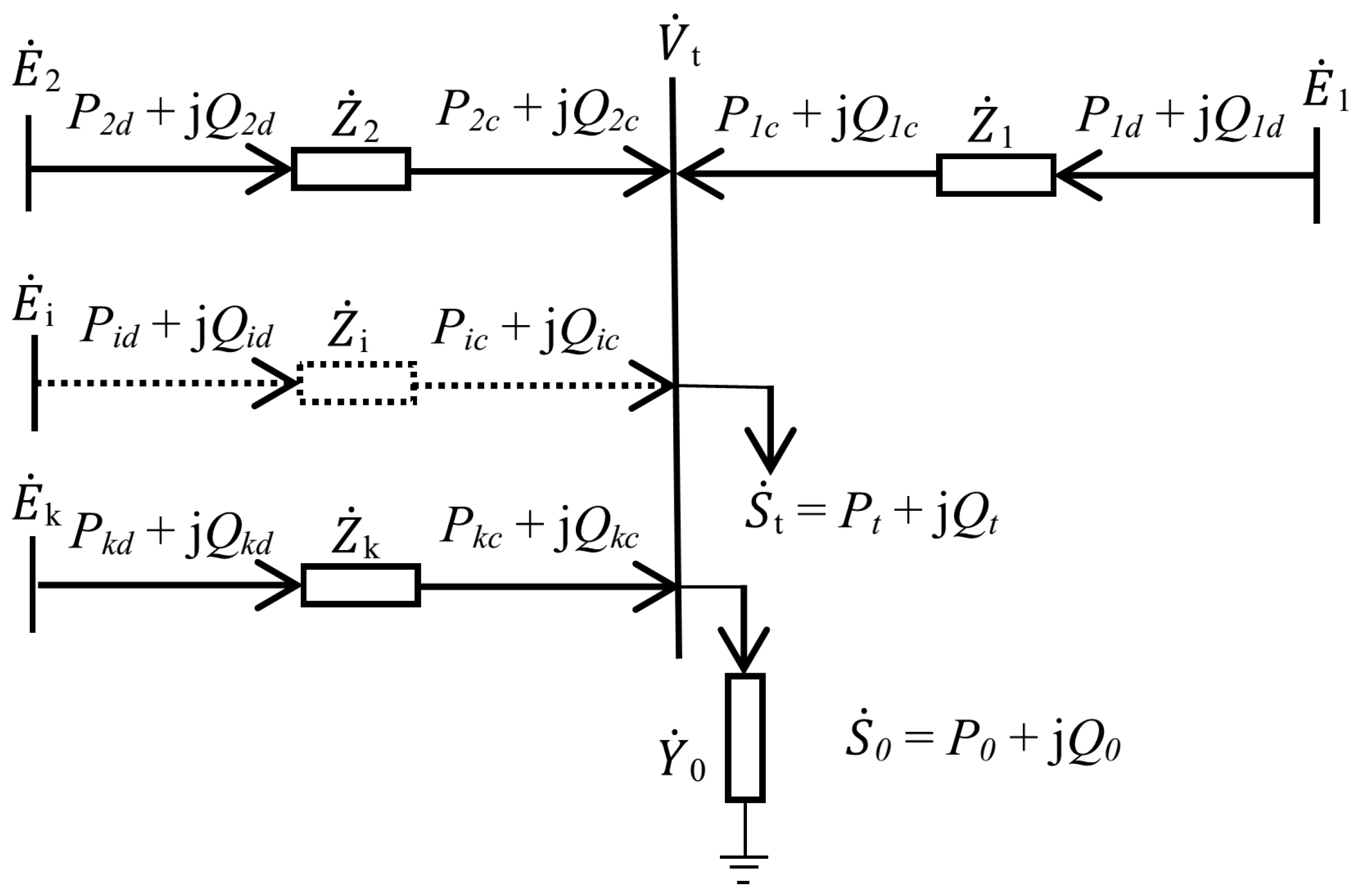
2.1. Determining Points on Stability Boundary

For assessing the stability of a power system, stability margins are often used, i.e., KP = [(PlimP0)/P0] × 100% and KQ = [(QlimQ0)/Q0] × 100%, where KP and KQ are the stability reserve ratios, Plim and Qlim are the values of limitation, and P0 and Q0 are the values at the operating points for active and reactive power, respectively (see Figure 1). The determination of Plim and Qlim for buses is based on completely conventional conditions; for example, Pj of bus j is considered to ascend to the limit, while all remaining parameters are constant [13]. Such determination is different from the actual variation of parameters in operation. Suppose that the characteristics of stability limit of bus j is assumed to be determined in the power plane, as in Figure 1, in which if Qj is constant, the reserve capacity according to Pj is proportional to distance a, or if cos ϕi is constant, it is proportional to distance b, while the parameters may vary with distance c in reality. Thus, for the evaluation of the stability reserve, it is needed to determine the reserve according to the shortest distance d from the operating point to the stability boundary. The challenge is to calculate and draw the characteristics curve under static stable limit conditions to determine the operating region on the power plane, taking into account nonlinearities.
In this section, the pragmatic criterion dQ/dV presented in [21] is used to construct the permissible operating region on a power plane under the conditions of a static stability limit. The operating states of a power system can be assessed based on dQ/dV, i.e., if dQ/dV is negative, the system is stable; otherwise, the system is unstable. Based on this criterion, we develop a mathematical formulation to determine points on the boundary (i.e., determine a curve on the power plane) between stable and unstable states of the system, and then we use this boundary to separate the operating regions into two regions, i.e., stable and unstable regions on the power plane, and assess its stability.
Suppose that a power system has n buses in which there are k generation buses (among k generation buses, Bus 1 is the slack bus of the system). The system is represented by an equivalent diagram, and then an adopted Gaussian elimination method [22] is used to simplify the diagram to a simple one that includes k generation buses and the load bus considered, as shown in Figure 2. It is worth noting that, thanks to this technique, the proposed methodology in this paper can be effectively applied for large-scale power systems.
  • Ei is the electromotive force of generators connected at the ith generation bus (i = 1 ÷ k);
    Z ˙ i = R i + j X i is the equivalent impedance of the branch connecting generation bus i and the considered load at bus t;
  • Pid and Qid are the real and reactive power transferred from generation bus i to the considered load at bus t and before equivalent impedance Z ˙ i , respectively;
  • Pic and Qic are the real and reactive power transferred from generation bus i to the considered load at bus t and after equivalent impedance Z ˙ i , respectively;
  • Pt, Qt, and St are the real, reactive, and apparent power of the considered load at bus t;
  • Y ˙ 0 is the equivalent admittance-to-ground at the considered load bus t, Y ˙ 0 = 1 / Z ˙ 0 , where Z ˙ 0 = R 0 + j X 0 is the corresponding equivalent impedance;
  • P0, Q0, and S0 are the real, reactive, and apparent power transferred through Y ˙ 0 .
The mathematical formulation for determining points on a stability boundary is as follows.
Based on the power balance conditions at the load bus, we have:
{ Q t + Q 0 = Q 1 c + i = 2 k Q i c P t + P 0 = P 1 c + i = 2 k P i c
so:
{ Q t = ( Q 1 c Q 0 ) + i = 2 k Q i c P 1 c = ( P t + P 0 ) i = 2 k P i c
where:
P 0 = G V t 2 ; Q 0 = B V t 2 G = R 0 R 0 2 + X 0 2 ; B = X 0 R 0 2 + X 0 2
The power transferred from generation bus i to the considered load bus can be calculated using electromotive force E ˙ i and voltage at the load bus V ˙ i . The equations for calculating the active and reactive power transferred to the end of branch i are as follows
{ (4a) P i c = V t 2 Z i sin α i + E i V t Z i sin ( δ i + α i ) (4b) Q i c = V t 2 Z i cos α i + E i V t Z i cos ( δ i + α i )
where, Ei and Vi are magnitudes of E ˙ i and V ˙ i , respectively; δi is the angle difference between E ˙ i and V ˙ i ; and αi is the phase angle of Z ˙ i .
From Equations (4a) and (4b), Qic is deduced as follows:
Q i c = E i 2 V t 2 Z i 2 ( P i c + V t 2 Z i sin α i ) 2 V t 2 Z i cos α i
where:
Z i = R i 2 + X i 2 ; α i = π 2 arctg X i R i
From Equations (2), (3), and (5), the reactive power at the load bus is computed as follows:
Q t = E 1 2 V t 2 Z 1 2 ( ( P t + G V t 2 ) 2 k P i c + sin α 1 Z 1 V t 2 ) 2 + + 2 k E i 2 V t 2 Z i 2 ( P i c + sin α i Z i V t 2 ) 2 ( cos α 1 Z 1 + B + 2 k cos α i Z i ) V t 2
From the formula to calculate the active power at two endings of branch i, Pic, corresponding to the parameters of the operation modes, can be deduced as:
P i d = E i 2 Z i sin α i + E i V t Z i sin ( δ i α i )
so:
sin ( δ i α i ) = ( P i d E i 2 Z i sin α i ) Z i E i V t
We perform some trigonometric transformations as follows:
sin ( δ i + α i ) = sin [ ( δ i α i ) + 2 α i ] sin ( δ i + α i ) = sin ( δ i α i ) cos 2 α i + sin 2 α i cos ( δ i α i ) sin ( δ i + α i ) = sin ( δ i α i ) cos 2 α i + sin 2 α i 1 sin 2 ( δ i α i )
From Equations (4a), (7), and (8), we can determine Pic as:
P i c = V t 2 Z i sin α i + ( P i d E i 2 Z i sin α i ) cos 2 α i + sin 2 α i E i 2 V t 2 Z i 2 ( P i d E i 2 Z i sin α i ) 2
As can be seen from Equations (4a) and (6), the reactive power at the load bus Qt is a function of the voltage at load bus Vt:
Q t = f ( V t )
If there is a fluctuation of voltage at the load bus, it will lead to an imbalance of power. The amount of imbalance of reactive power can be identified as follows:
Δ Q = Q G Q T = f ( V t ) Q t
where QΣG is the total reactive power transferred to the load bus from all generators in the system; QΣT = Qt + Q0.
Taking the derivative of both sides of the above equation with respect to Vt, we obtain:
d Δ Q d V t = d f ( V t ) d V t d Q t d V t
Suppose that Qt varies very little with the variation of Vt, so:
d Q t d V t = 0 d Δ Q d V t = d f ( V t ) d V t
According to pragmatic criterion dQ/dV in [14], the system reaches its static stability limit when:
d Δ Q d V t = d f ( V t ) d V t = 0
The process for determining points on a stability boundary is implemented step by step as follows.
Step 1:
Suppose:
Q i min Q i d Q i max , i = 2 , k ¯
in which, Qimin and Qimax are the regulating limits for generating the reactive power of source i (limits of the regulator of an excitation system) and Qid is the reactive power at the first point of branch i. The nonlinear equations in Equation (10) are solved for voltage at the load bus in limited state Vt,lim. Qt is calculated by putting Vt,lim and a given value Pt into Equation (6). In order to conclude whether the point M (Qt, Pt) is located on the static stability limit of the system or not, it is needed to verify Hypothesis (11).
The reactive power at the first point of branch i can be calculated by using the following formula:
Q i d = E i 2 Z i cos α i ( E i V t , lim Z i ) 2 ( P i d E i 2 Z i sin α i ) 2
If all the generation buses satisfy Hypothesis (11), point M (Qt, Pt) will be located on the static stability limit of the system. In case there are m generators within their regulating limits and (k-m) ones exceeding their regulating limits,
Q i min Q i d Q i max    i = 2 , m ¯ Q j d Q j min   or   Q j d Q j max j = m + 1 , k ¯
Step 2:
For source j exceeding its regulating limit:
  • QjdQjmin set Qjd = Qjmin
  • QjdQjmax set Qjd = Qjmax
In this case, the reactive power transferred to load bus can be approximately determined:
{ Q j c = Q j d P j d 2 + Q j d 2 U j , r a t e d 2 X j = const P j c = P j d P j d 2 + Q j d 2 U j , r a t e d 2 R j = const
where Uj,rated denotes the rated voltage at bus j.
The formula to calculate the reactive power at load bus (6) can be changed as follows:
f ( V t ) = E 1 2 V t 2 Z 1 2 ( P t + G V t 2 + sin α 1 Z 1 V t 2 2 m P i c m + 1 k P j c ) 2 + 2 m E i 2 V t 2 Z i 2 ( P i c + sin α i Z i V t 2 ) 2 + k + 1 n Q j c ( B + cos α 1 Z 1 + 2 k cos α i Z i ) U t 2
where, Pic is calculated in Equation (9) and Pjc and Qjc are obtained from Equation (13).
Solving nonlinear Equation (10) we can obtain Vt,lim and f(Vt) (see (14)); continue to check m adjustable sources if there is any source violated. If there is no source violated, M(Qt, Pt) is located on the stability limit; otherwise, we recalculate Step 2.

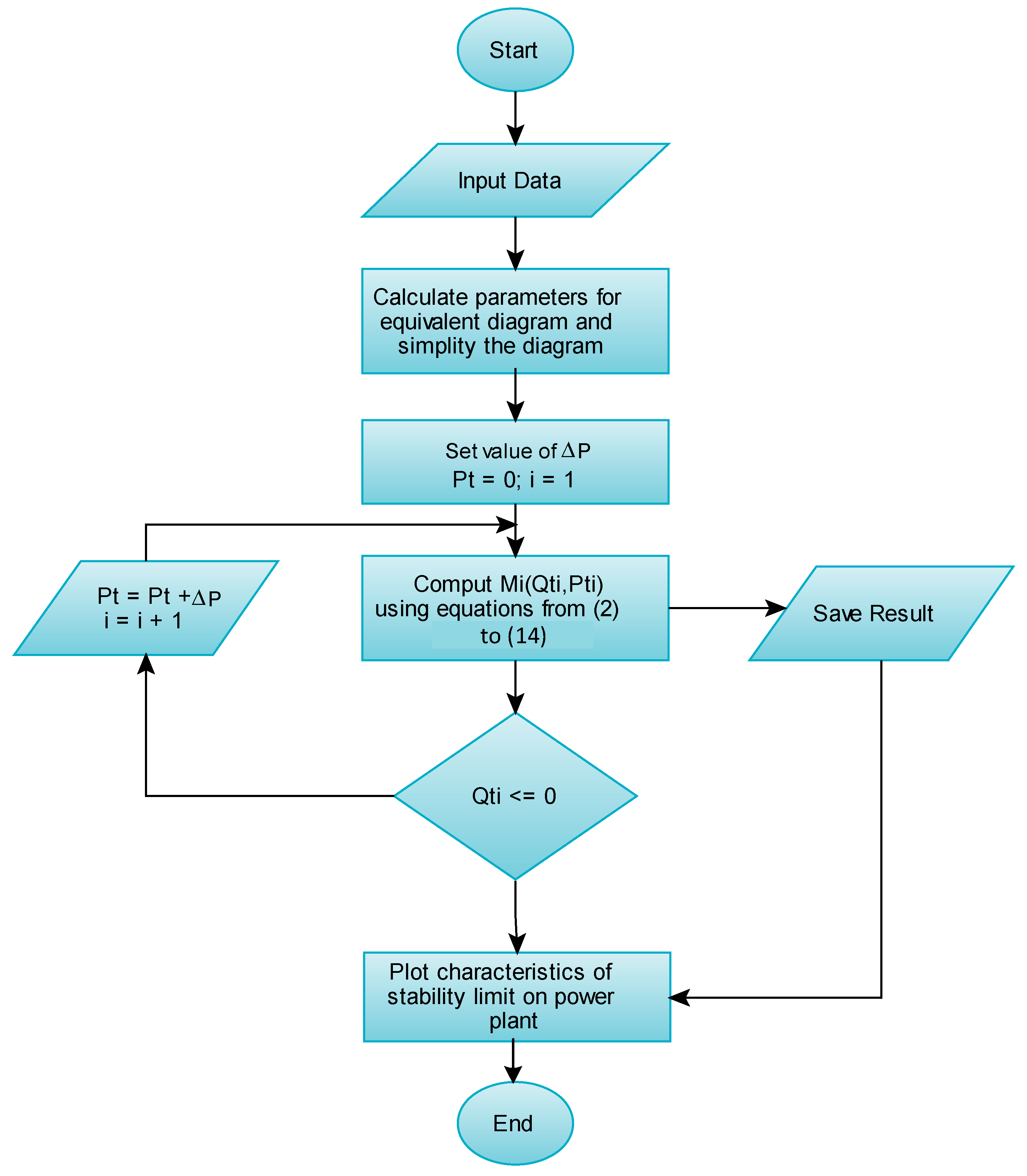
2.2. Development of Algorithm for Drawing Characteristics of Stability Limit

From the calculation for determining points located on the stability boundary in Section 2.1, we can build an algorithm for drawing the characteristics of the stability limit, as in Figure 3.

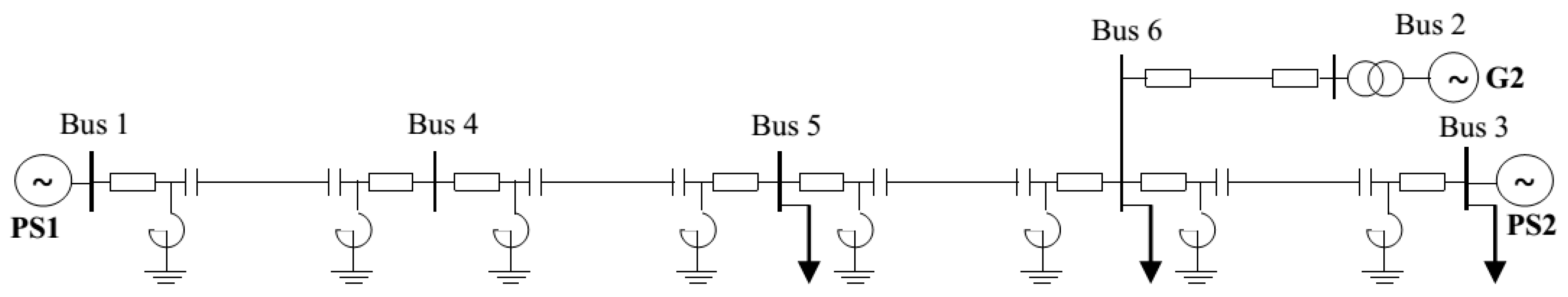
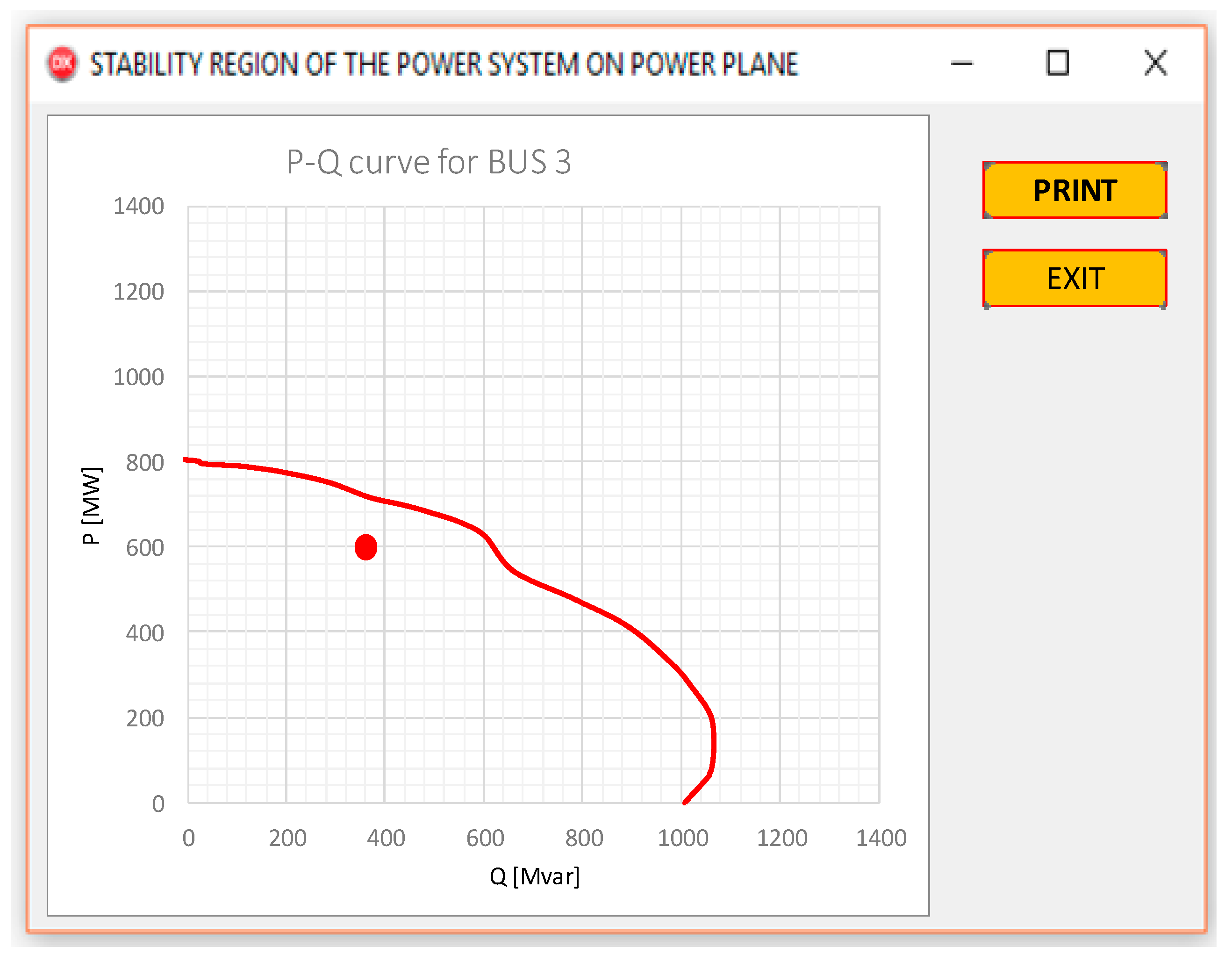
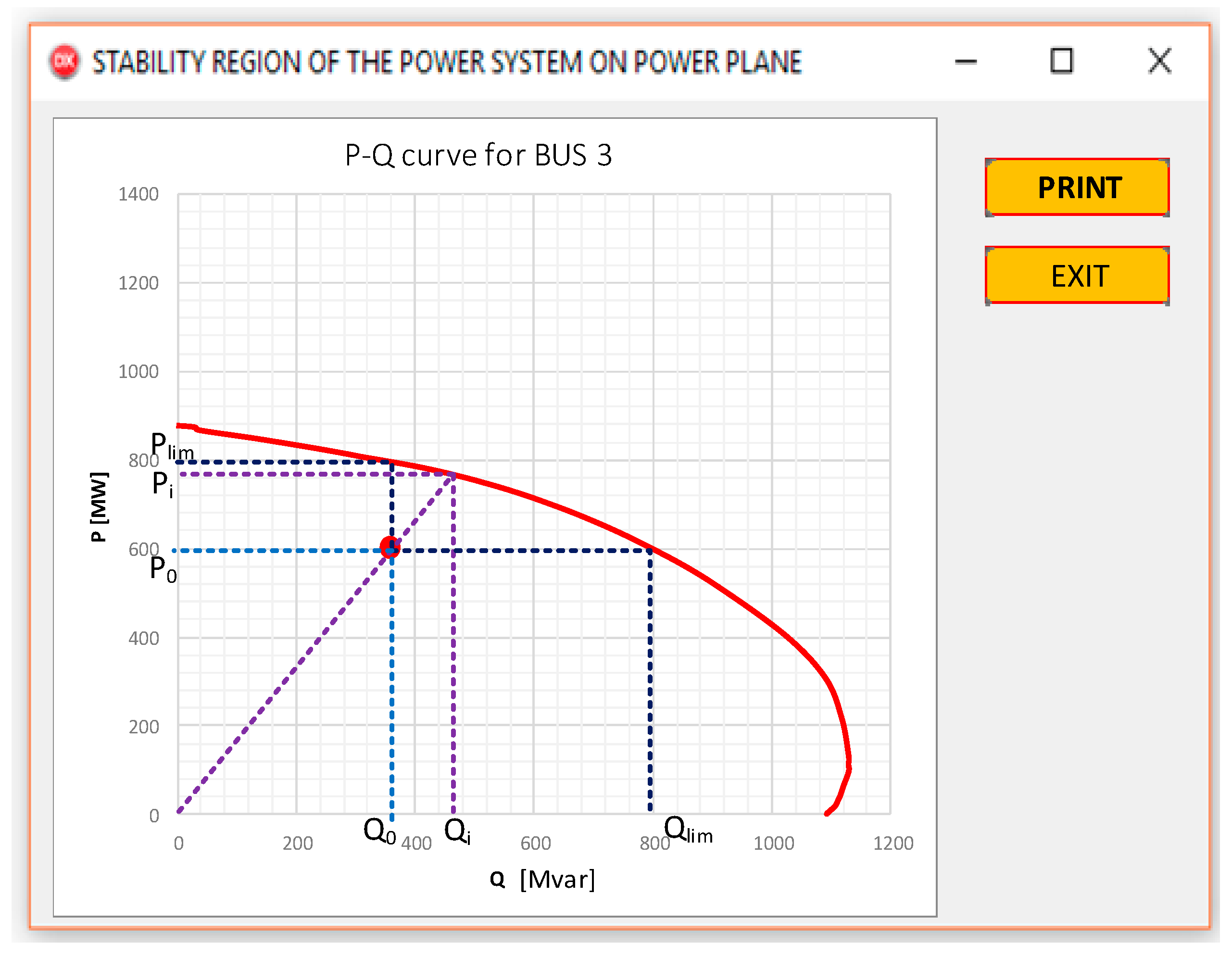
3. Application to Building a Program for Determining Permissible Operating Region of Power Systems on Power Plane

Based on the algorithm developed in Section 2, we build a procedure and then a computer program to determine the operating region of power systems using Delphi programming language. For the illustration, we run it for six-bus power system, as shown in Figure 4, in which Power System 2 (PS2) is connected to Power System 1 (PS1) with an unlimited capacity via a long-distance 500 kV UHV transmission line, in the middle of the line at Bus 6, to which a power plant (G2) is connected. In addition, there are two regional electricity networks with low capacity that are represented as two loads connected to Bus 5 and Bus 6. There is also a load connected to Bus 3.
PS1 has an unlimited capacity so the voltage at Bus 1 (U1) can be considered constant, and Bus 1 is considered the slack bus in the system. PS2 is represented by an electromotive force Eeq and an equivalent impedence Zeq. Therefore, the system considered can be represented by an equivalent diagram, as shown in Figure 5. From this equivalent diagram, the algorithm in Section 2 is applied to construct the characteristics of the stability limit on the power plane. The program is run for the test system with its initial interface, as in Figure 6.
For example, when clicking on Bus 3, the resulting P-Q curve is obtained, as shown in Figure 7 in which the circular point represents the operating point. In this case, the operating point belongs to the stable region (the region covered by two axes and the P-Q curve), indicating that the system is stable. If the load at Bus 3 is increased, exceeding P-Q curve (stability boundary), a warning message will appear to notify the user that the system is unstable, as in Figure 8.
Using the program, the permissible operating region at Buses 3, 5, and 6 can be investigated. Moreover, factors that affect the operating region at a load bus can be examined such as the power change at other load buses in the system, the change in power generated (e.g., P2f), the number of working units (change in Q2max) of the power plant connected to Bus 6, the change in power generated (P3f), and the limit of adjusting the reactive power Q3max of PS2. In order to identify the critical bus and factors affecting the stability of the system, the operating parameters are assumed to be set in the program, as in Table 1.
The operating regions at Buses 5, 6, and 3 are plotted in Figure 9, Figure 10 and Figure 11, respectively. By comparing the distances from the operating points to the P-Q curves for all load buses in the system, the most dangerous bus can be identified. In this system, Bus 3 is found to be the most dangerous one that needs to be carefully supervised during the operation of the system.
In particular, while surveying the operating region at Bus 3, as in Figure 11, we decrease Q3max from 1150 Mvar to 1000 Mvar; the characteristics of stability limit will be changed, as shown in Figure 12. In other cases, we adjust P2f from 360 MW to 240 MW, for which the characteristics of stability limit are shown in Figure 13, or we adjust the load at Bus 6 from P6 + jQ6 = 400 + j240 MVA to P6 + jQ6 = 500 + j360 MVA, so that the curve will be obtained as in Figure 14. Thus, by adjusting the operating parameters and observing the change in the P-Q curve, we can find effective solutions to improve the stability of the system.
Extensive testing on the above six-bus system indicates the good performance of the proposed approach in comparison with the results obtained by other commercial software that includes functions for power system stability studies. For example, Figure 15 shows the operating region at Bus 3 and the determination of values for calculating the stability reserve ratios, while Table 2 gives the results obtained by the proposed method compared with the results from the Power System Simulator for Engineering (PSS/E) software. It should be noted that the curve we build and the stability reserve ratios that are computed are realistic because we construct the curve point-by-point without using any assumption about the shape of the curve or assumption about the change of load. As illustrated in Figure 15, when surveying the operating region at a certain load bus (e.g., Bus 3), from the operating point of the load and the characteristics curve under the static stable limit built, the stability reserve ratios can be computed as follows. At the operating point, P0 and Q0 are known; then S0 is calculated as S 0 = P 0 2 + Q 0 2 . To determine the limitation of Q (Qlim in Figure 15), P is kept constant (P = P0), while Q is increased until it reaches the curve. Analogously, Plim is determined by increasing P until it reaches, the curve whilst Q is held constant (Q = Q0). Maintaining constant cosϕ and increasing S (i.e., increasing both P and Q along the line that crosses the origin point and the operating point in Figure 15) until it reaches the curve, Pi and Qi are found out and Si is calculated as S i = P i 2 + Q i 2 . Eventually, stability reserve ratios KP, KQ, and KS are computed:
KP = [(PlimP0)/P0] × 100%; KQ = [(QlimQ0)/Q0] × 100%; KS = [(SiS0)/S0] × 100%
Using the above formulas, results are obtained as shown in Table 2.
The proposed method is implemented on an Intel Core i5 CPU 2.3 GHz/4.00 GB RAM PC (Computer Dell Vostro 14-5459, Core i5 6200U, Manufacturer: Dell Inc., Chengdu, China), taking 3 × 10⁻³ s, 5 × 10⁻³ s, and 0.11 s for the above six-bus system, IEEE (The Institute of Electrical and Electronics Engineers) nine-bus system, an IEEE 118-bus system [23], respectively. Hence, the proposed approach can be run and can quickly provide results, showing that it can be used for real-time analysis, thanks to the use of an analytical approach in developing the algorithm in this paper.

4. Conclusions

In this paper, we present a methodology for constructing the characteristics of the stability limit of the system according to the static stability conditions on a power plane. Based on the proposed algorithm, a procedure and a program are built and real-time analysis can be performed; the program can be run and quickly provide results (e.g., it needs only 0.11 s for an IEEE 118-bus system with an Intel Core i5 CPU 2.3 GHz/4.00 GB RAM PC) thanks to our use of an analytical approach to develop the algorithm.
With the above-mentioned attractive feature, the proposed approach and the program developed based on it can be applied to a practical power system to monitor its stability reserve in a real-time environment by using online data acquisition systems to provide the necessary information about the system and its operating parameters.
When surveying the operating region of the load buses in the system, by observing the distances from the operating points to the stability boundaries, the operator can easily identify the most critical buses in the system, which should then be carefully monitored during the operation. For example, for the six-bus power system considered in Section 3, Bus 3 is found to the most critical one (Figure 11 for Bus 3 compared to Figure 9 for Bus 5 and Figure 10 for Bus 6).
In addition, by observing the change in the characteristics of the stability limit (P-Q curve) when adjusting operating parameters such as the consumption capacity at the load bus, the power output from power plants, the number of operating units in the system, etc., the most efficient solution for raising the stability reserve of the system can be indicated.
One more important point that should be noted about the proposed methodology is that the curve we build, as presented in Section 2, is realistic since we construct it point-by-point without using any assumption about the shape of the curve or any assumption about the change of load either.

Acknowledgments

All sources of funding of the study should be disclosed. Please clearly indicate grants that you have received in support of your research work. Clearly state if you received funds for covering the costs to publish in open access.

Author Contributions

Van Duong Ngo, Dinh Duong Le, Kim Hung Le, and Van Kien Pham developed the algorithm for drawing the characteristics of the stability limit. Van Duong Ngo and Van Kien Pham created the computer program for determining the operating regions of power systems. Van Duong Ngo, Kim Hung Le, Van Kien Pham, Dinh Duong Le, and Alberto Berizzi analyzed the results. Van-Duong Ngo and Dinh Duong Le wrote the paper. Alberto Berizzi coordinated the main theme of this paper and thoroughly reviewed the paper.

Conflicts of Interest

The authors declare no conflict of interest.

References

  1. Kundur, P.; Paserba, J.; Ajjarapu, V.; Andersson, G.; Bose, A.; Canizares, C.; Hatziargyriou, N.; Hill, D.; Stankovic, A.; Taylor, C.; et al. Definition and classification of power system stability IEEE/CIGRE joint task force on stability terms and definitions. IEEE Trans. Power Syst. 2004, 19, 1387–1401. [Google Scholar]
  2. Oluic, M.; Ghandhari, M.; Berggren, M. Methodology for Rotor Angle Transient Stability Assessment in Parameter Space. IEEE Trans. Power Syst. 2017, 32, 1202–1211. [Google Scholar] [CrossRef]
  3. Meegahapola, L.; Littler, T. Characterisation of large disturbance rotor angle and voltage stability in interconnected power networks with distributed wind generation. IET Renew. Power Gen. 2015, 9, 272–283. [Google Scholar] [CrossRef]
  4. Jóhannsson, H.; Nielsen, A.H.; Østergaard, J. Wide-area assessment of aperiodic small signal rotor angle stability in real-time. In Proceedings of the 2014 IEEE PES General Meeting, National Harbor, MD, USA, 27–31 July 2014. [Google Scholar]
  5. Hatziargyriou, N.; Karapidakis, E.; Hatzifotis, D. Frequency stability of power systems in large islands with wind power penetration. In Proceedings of the Bulk Power System Dynamics Control Symposium-IV, Restructuring, Santorini, Greece, 24–28 August 1998. [Google Scholar]
  6. Hu, J.; Cao, J.; Guerrero, J.M.; Yong, T.; Yu, J. Improving Frequency Stability Based on Distributed Control of Multiple Load Aggregators. IEEE Trans. Smart Grid 2017, 8, 1553–1567. [Google Scholar] [CrossRef]
  7. Taylor, C.W. Power System Voltage Stability; McGraw-Hill Inc.: New York, NY, USA, 1994. [Google Scholar]
  8. Modarresi, J.; Gholipour, E.; Khodabakhshian, A. A comprehensive review of the voltage stability indices. Renew. Sust. Energ. Rev. 2016, 63, 1–12. [Google Scholar] [CrossRef]
  9. Karbalaei, F.; Soleymani, H.; Afsharnia, S. A comparison of voltage collapse proximity indicators. In Proceedings of the International Power Electronics Conference (IPEC), Singapore, 27–29 October 2010. [Google Scholar]
  10. Clark, H.K. New challenge: Voltage stability. IEEE Power Eng. Rev. 1990, 19, 30–37. [Google Scholar]
  11. Gupta, R.K.; Alaywan, Z.A.; Stuart, R.B.; Reece, T.A. Steady state voltage instability operations perspective. IEEE Trans. Power Syst. 1990, 5, 1345–1354. [Google Scholar] [CrossRef]
  12. Pourbeik, P.; Meyer, A.; Tilford, M.A. Solving a Potential Voltage Stability Problem with the Application of a Static VAr Compensator. In Proceedings of the IEEE Power Engineering Society General Meeting, Tampa, FL, USA, 27–31 January 2007; pp. 1–8. [Google Scholar]
  13. Kundur, P. Power System Stability and Control; McGraw-Hill Inc.: New York, NY, USA, 1994. [Google Scholar]
  14. Toma, R.; Gavrilaș, M. Voltage Stability Assessment for Wind Farms Integration in Electricity Grids with and without Consideration of Voltage Dependent Loads. In Proceedings of the International Conference and Exposition on Electrical and Power Engineering (EPE 2016), Iasi, Romania, 20–22 October 2016. [Google Scholar]
  15. Rawat, M.S.; Vadhera, S. Analysis of wind power penetration on power system voltage stability. In Proceedings of the IEEE 6th International Conference on Power Systems (ICPS), New Delhi, India, 4–6 March 2016. [Google Scholar]
  16. Balamourougan, V.; Sidhu, T.; Sachdev, M. Technique for online prediction of voltage collapse. IEE Proc.-Gener. Transm. Distrib. 2004, 151, 453–460. [Google Scholar] [CrossRef]
  17. Zhang, P.; Min, L.; Chen, J. Measurement Based Voltage Stability Monitoring and Control. U.S. Patent Application No. US 2009/0299664A1, December 2009. [Google Scholar]
  18. Cutsem, T.V.; Vournas, C. Voltage Stability of Electric Power Systems; Kluwer Academic: Boston, MA, USA, 1998. [Google Scholar]
  19. Glavic, M.; Lelic, M.; Novosel, D.; Heredia, E.; Kosterev, D. A Simple Computation and Visualization of Voltage Stability Power Margins in Real-Time. In Proceedings of the IEEE PES Transmission and Distribution Conference and Exposition (T&D), Orlando, FL, USA, 7–10 May 2012; pp. 1–7. [Google Scholar]
  20. Lin, Y.Z.; Shi, L.B.; Yao, L.Z.; Ni, Y.X.; Qin, S.Y.; Wang, R.M.; Zhang, J.P. An Analytical Solution for Voltage Stability Studies Incorporating Wind Power. J. Electr. Eng. Technol. 2015, 10, 30–40. [Google Scholar] [CrossRef]
  21. Machowski, J.; Bialek, J.W.; Bumby, J.R. Power System Dynamics and Stability; John Wiley & Sons Ltd.: Chichester, UK, 1997. [Google Scholar]
  22. Pham, V.K.; Ngo, V.D.; Le, D.D.; Huynh, V.K. Studying and building program for simplifying electrical network diagram using Gaussian elimination algorithm. J. Sci. Technol. Univ. Danang 2015, 6, 24–28. [Google Scholar]
  23. Power System Test Case Archive. Available online: https://www2.ee.washington.edu/research/pstca/pf118/pg_tca118bus.htm (accessed on 6 February 2017).
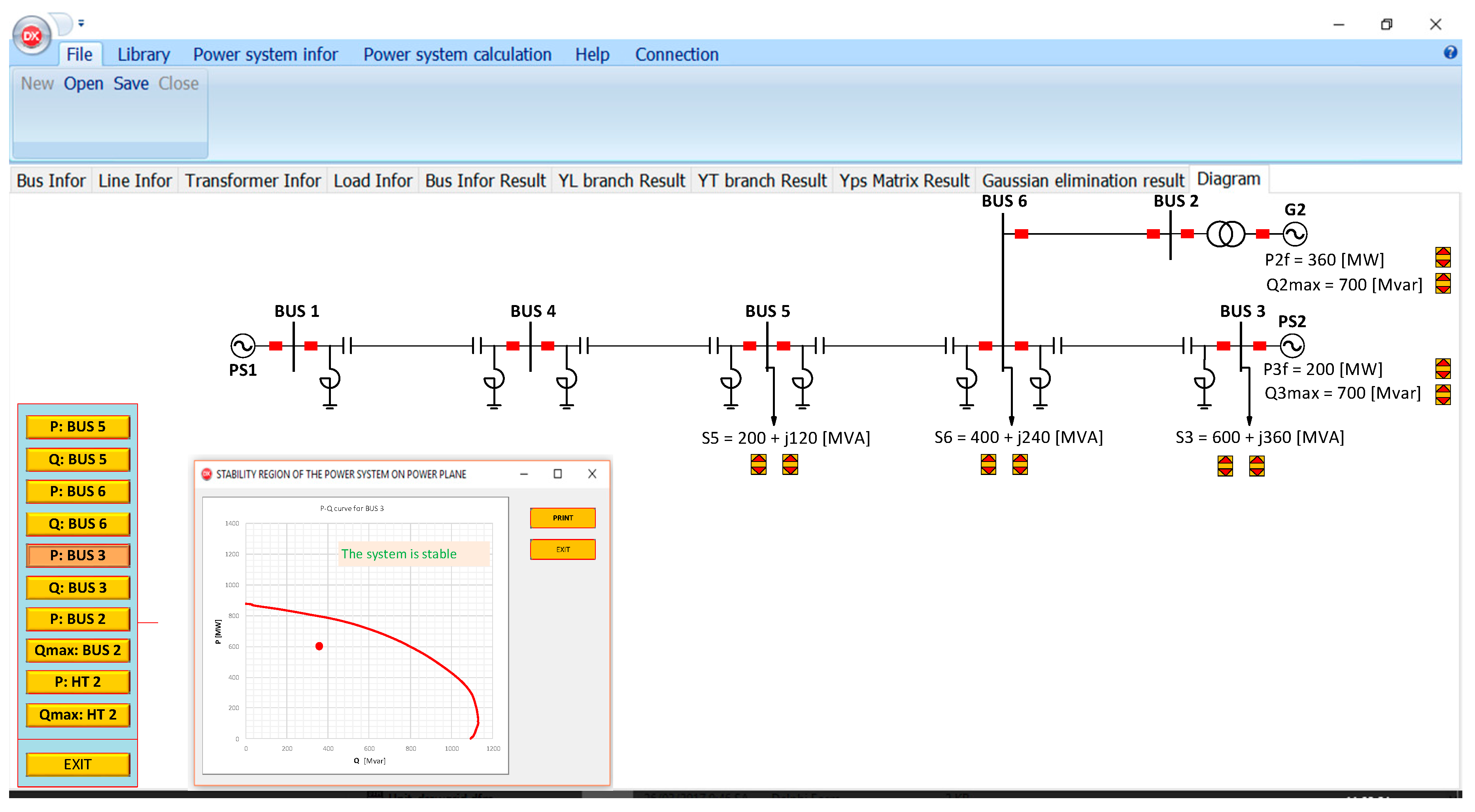
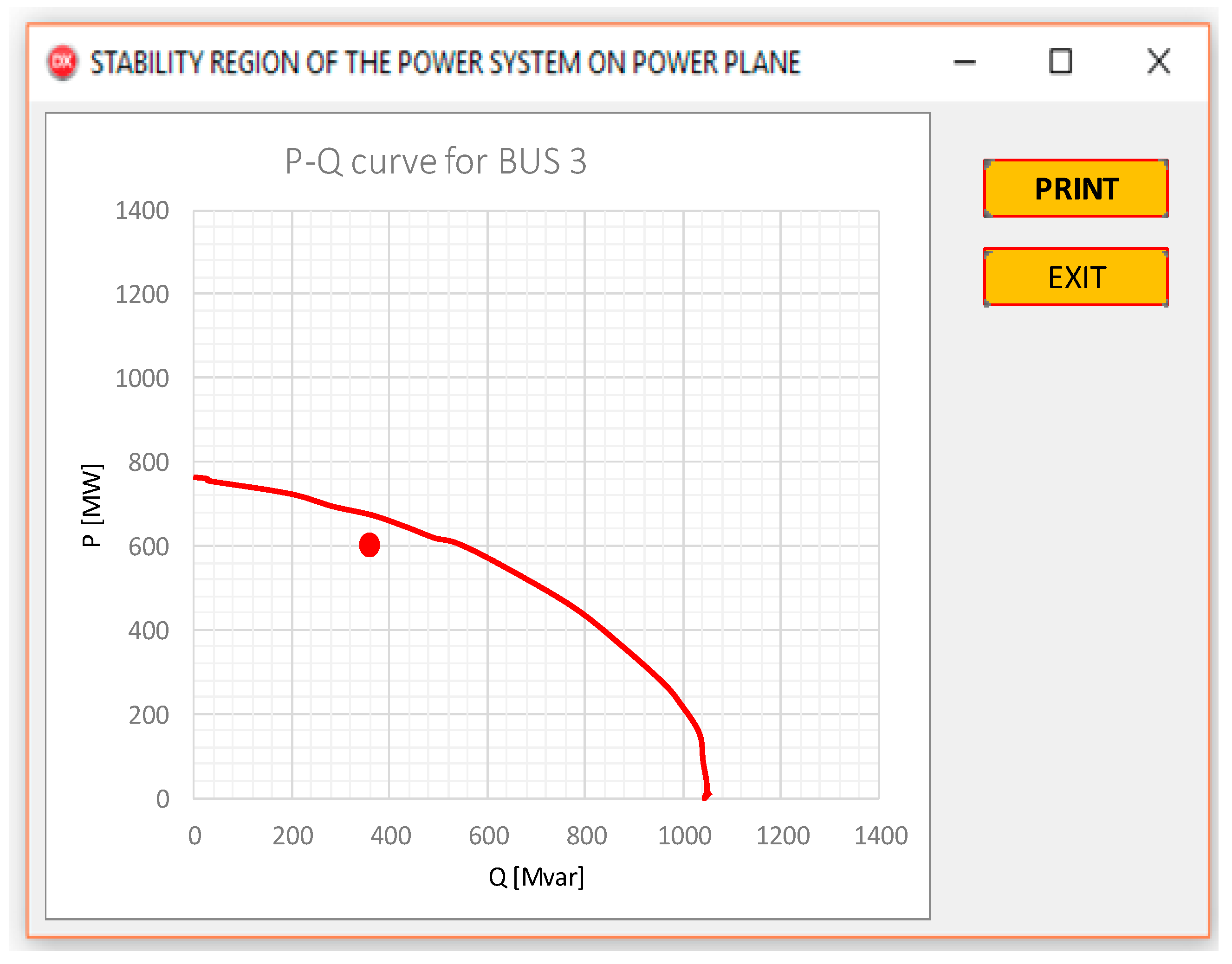
Figure 1. P-Q curve on power plane.
Energies 10 01163 g001
Figure 2. Simplified equivalent diagram.
Energies 10 01163 g002
Figure 3. Algorithm for drawing the characteristics of the stability limit.
Energies 10 01163 g003
Figure 4. Six bus power system.
Energies 10 01163 g004
Figure 5. Equivalent diagram of the six bus power system.
Energies 10 01163 g005
Figure 6. Diagram of the six-bus power system in the program.
Energies 10 01163 g006
Figure 7. P-Q curve plotted for Bus 3 in a stable state.
Energies 10 01163 g007
Figure 8. P-Q curve plotted for Bus 3 in an unstable state.
Energies 10 01163 g008
Figure 9. Operating region at Bus 5.
Energies 10 01163 g009
Figure 10. Operating region at Bus 6.
Energies 10 01163 g010
Figure 11. Operating region at Bus 3.
Energies 10 01163 g011
Figure 12. Operating region at Bus 3 when adjusting Q3max.
Energies 10 01163 g012
Figure 13. Operating region at Bus 3 when adjusting P2f.
Energies 10 01163 g013
Figure 14. Operating region at Bus 3 when adjusting the load at Bus 6.
Energies 10 01163 g014
Figure 15. Calculating the stability reserve ratios for the operating region at Bus 3.
Energies 10 01163 g015
Table 1. Operating parameters for the six-bus test system.
Bus 3Bus 5Bus 6Q2max (Mvar)P2f (MW)Q3max (Mvar)P2f (MW)
P (MW)Q (Mvar)P (MW)Q (Mvar)P (MW)Q (Mvar)
600360200120400240700360700200
Table 2. Comparison of the results.
ParamatersComparison of Results
Proposed ApproachPSS/E
P0 (MW)600600
Q0 (Mvar)360360
S0 (MVA)699.7699.7
Plim (MW)800833
Qlim (Mvar)800821
Pi (MW)772791
Qi (Mvar)448475
Si (MVA)892.6923
KP (%)27.531.8
KQ (%)33.438.8
KS (%)122.3128

