Abstract
The reconfigurable power electronic converters (RPECs) are a new generation of systems, which modify their physical configuration in terms of a desired input or output operation characteristic. This kind of converters is very attractive in terms of versatility, compactness, and robustness. They have been proposed in areas such as illumination, transport electrification (TE), eenewable energy (RE), smart grids and the internet of things (IoT). However, the resulting converters operate in switched variable operation-regions, rather than over single operation points. As a result, there is a complexity increment on the modeling and control stage such that traditional techniques are no longer valid. In order to overcome these challenges, this paper proposes a kind of switched polytopic controller (SPC) suitable to stabilize an RPEC. Modeling, control, numerical and practical results are reported. To this end, a 400 W positive synchronous bi-directional buck/boost converter is used as a testbed. It is also shown, that the proposed converter and robust controller accomplish a compact, modular and reliable design during different working configuration, operation points and load changes.
1. Introduction
Power electronic converters (PECs) are used in applications where an efficient energy conversion is required by using solid-state devices [1]. The application range can differ from a fraction of a Watt to millions of Watts, and several disciplines interact in its different development stages (modeling, control, numerical simulation, implementation design, and performance evaluation) such as electric circuits, digital electronics, computer-aided design, control theory, among others [2]. Nowadays, there is an interest to develop portable and high-power density PECs, which has resulted in a new trend of PEC called Reconfigurable PECs (RPECs). Examples of those systems can be found in different applications, for instance:
- Illumination: RPECs for the power factor correction and for a light emitting diode (LED) driver design were reported in [3,4,5], and for a high-pressure sodium lamp driver design in [6].
- Transport electrification (TE): RPECs have been applied in: (a) the charger stage [7,8,9,10,11]; (b) starter/generator [12]; (c) battery [13,14,15,16,17,18]; (d) suspension [19]; and (e) propulsion [20,21,22].
- Renewable energy (RE): RPEC examples can be found in: photovoltaic [23,24,25,26,27,28,29,30,31], eolic [32], residential storage (batteries bank) [33,34] and fuel cell [35] systems.
- Smart grid: RPECs have been reported on microgrid [36,37,38] and picogrid [39,40] applications.
- Internet of things (IoT): An RPEC focused on low cost and low size power supply was reported on [41].
It can be noticed that, besides its final application, motivations to develop this kind of PEC relies on one or more of the following characteristics: (a) versatility; (b) compactness; (c) robustness against load variation; and (d) significant input and output changes.
However, the design of an RPEC implies a significant increment of control complexity. This last, due to that the converter does not stabilize anymore in operation points over a single operation region, instead, it must stabilize in operating points over operation regions that switch over time [42]. To this end, some authors had proposed several control syntheses such as intelligent [43], linear quadratic [44], passivity-based [45] by pulse adjustment [46] and hybrid controllers [47]. These techniques deal with local solutions (decoupled for each operation region) and not with a global one, which, in implementation terms, implies decoupling strategies and delays. Notice from now on that an RPEC can be analyzed as a polytopic switched system (PSS) [48] in order to gain global results.
One of the first uses of the polytopic representation was for modeling and controlling a diesel engine in several operation modes [49]. Silva et al. reported about sliding mode controllers, from a polytopic perspective, to cope with uncertainties in mathematical models and applied the analysis to an aircraft [50]. In [51], the authors performed a stability analysis for networked control systems using a polytopic system applied to a batch reactor. Huang et al. reported a polytopic parameter-varying model applied to a flexible air-breathing hypersonic vehicle; they divided the system into sub-regions, proposed a controller for each sub-region and switched between them to get closed-loop asymptotically stable local systems. A similar approach applied to unmanned aerial vehicles was reported in [52], but in both cases, the polytopic subsystems were considered adjacent simplifying the stability analysis. The case of asynchronous polytopic switching was addressed on [53] for a highly maneuverable vehicle; in such paper only numerical simulations were reported. A step-forward was reported on [54], where the robust fault-tolerant tracking control case, for a nonlinear networked system under asynchronous switching was investigated. After, the stability of a switched linear system with polytopic uncertainties applied to a servomechanism system was reported on [55].
The case of a switched linear parameter varying (SLPV) system was reported on [56]. In this paper, a new finite time stability condition and a robust finite time controller were reported. The analysis and controller considered the case of an SLPV system with two dissimilar uncertainty modeling assumptions, that they used to benchmark the attitude control of bank-to-turn missiles. On another hand, an SLPV with bounds on control and state was addressed in [57]. This paper reported the controller synthesis and closed-loop stability under polytopic uncertainties for three numerical examples.
A stability analysis using Lyapunov functions for a PEC modeled as a polytopic switched system was early reported in [58]. The idea of a polytopic black box modeling, applied to an unregulated DC bus and a Flyback DC-DC converter, was introduced in [59] including numerical and practical results. The main idea was to get local models validated at different operation conditions by using a nonlinear interpolation, the local models were interlaced by means of their adjacent operating point. A black-box large-signal stability analysis based on Lyapunov was reported on [60]. In such paper, constant power loads in a microgrid are considered, and results show that the stability region achieved by this method was analogous to analytical linear methods, but the resulting analysis is comparatively complex. A further step in the modeling of RPEC was given in [61], where a DC- polytopic model was reported, and numerical results of the switching behavior in the black box model were reported. A related analysis applied to smart grid was proposed in [62]; in this paper just simulation results for a PV, battery and grid converter was considered. A non-linear behavior modeling, based on a look-up table and a polytopic structure, was reported on [63]. In such paper, the cascade and parallel configuration connected to an electronic load was modeled in terms of their G-parameters; numerical and experimental results are presented for two commercial DC-DC converters.
It can be noticed that most of the above works are contributions related to PECs and not to RPECs, which is the main contribution of this work. In this paper, a switched polytopic controller for the RPEC reported in [64] is proposed. This RPEC was developed to provide a unique, low-cost, and stable solution to several problems arising in Electric Vehicles and smart grid scenarios. For example, in an EV it is desirable a single solution to driving the power from the battery to the main motor (Mode I), or from a fuel cell (mode II), recharge the battery when regenerative braking is active (Mode III), slow recharge of the battery (Mode IV), and fast charge when a high voltage is available (Mode V). This topology involves less components than separated solutions to each of the mentioned problems. The proposed converter and controller accomplishes a compact, modular and reliable design. The operation principle is analyzed at different working operation modes using idealized waveforms, fixed frequency, and continuous conduction mode. In addition, it is also shown numerical and practical results obtained with a 400 W testbed prototype.
2. Modeling
The proposed RPEC has two input voltages and in addition to the battery which also acts as a storage element. By managing a switching strategy, the power flow between a source and the battery/load is possible, as well as bidirectionally between the battery and the load. The circuit topology of the converter is shown in Figure 1. There are three switches allowing conduction to each of the sources and the load, and five power switches. The possible switching combinations that are able to perform result in five operation modes. These are modeled as follows.
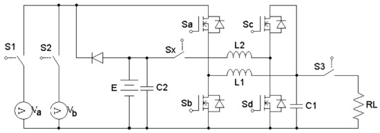
Figure 1.
Proposed testbed.
2.1. Mode I (Buck)
In Figure 2 is shown the schematic diagram for the Mode I; the circuit corresponds to a well known Buck converter when , , , and are open and is closed. and are switched alternately and voltage E is supplied to the branch at high frequency when a non-zero voltage at is needed. Mosfets and are modeled as variable resistances (Figure 3) with smooth transitions from very high to very low resistance and vice versa.
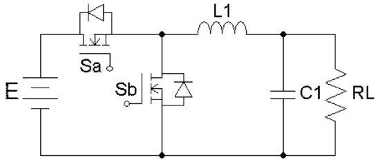
Figure 2.
Mode I Schematic.
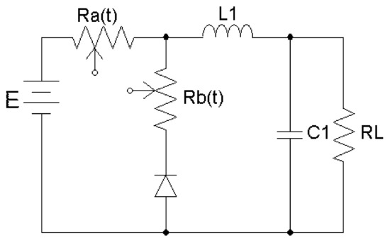
Figure 3.
Idealized Mode I Schematic.
This is, when the Mosfet is in conducting state, activated by a proper gate signaling, a very low resistance between their switch terminals (Drain-Source) is presented, while the Mosfet is in a non-conducting state, by a proper gate signaling, such that resistance between their switching terminals is of a high value. Analogously, when Mosfet is in conducting state, the resistance between their switch terminals is low, while the resistance between switching terminals of Mosfet is high.
The transitions are alternately modulated at a fixed frequency (PWM) in continuous mode with dead-time, which depends on the characteristic switching times of the Mosfets, and it is considered for the analysis as negligible; this is, in order to avoid their simultaneous conduction (Figure 3). In such idealization, the voltage supplied to the branch can be taken as the average of a smooth time function (Figure 4):
where
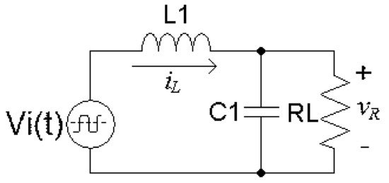
Figure 4.
Idealized Mode I Schematic.
This is, as the Mosfets are modeled as variable resistances, the voltage is obtained from a resistances arrangement that can be seen as a voltage divider of E, and represents the PWM duty-cycle. Note that the values of the real resistances depend on the electronic device (Mosfet) and cannot be set by u (unless an averaged point of view were used); this is only an idealization to perform the modeling of the circuit and the only modifiable parameter is the PWM duty cycle. The equations that describe the dynamic behavior are:
Note that the System (3), (4) coincides with the well known averaged model of the buck converter ([65,66], et al.) as well as with the following dynamic models of this section. The equivalent representation in state space is:
where , denotes the matrix transpose operation and
In the following, the model (5) is addressed as nominal since in this work all of the model parameters are considered time varying values. Using parametric ranges of uncertainty, a polytopic description is obtained as follows: consider that , ; this is, the inductance varies in a known range from a maximum to a minimum inclusive. Similarly and . Then, a Linear Parameter Varying system (LPV) representation is:
where ; this is, matrices y are polytopic in the following sense:
where is known as a simplex and or equivalently:
where represents the minimum possible value of the matrix entry for all the combinations of maximum and minimum values of the parameters and represents the maximum possible value of the matrix entry for all the combinations of maximum and minimum values of the parameters and so on.
In other words, the system is now represented/rewritten as a polytopic one, and now the variation ranges are of unitary values of (simplex) instead of the full range of each parameter. Such construction is necessary to perform the stability analysis in the following sections. The matrices in the right side of (10) are known as vertexes. Similarly for :
2.2. Mode II (Boost)
In Figure 5 is shown the equivalent schematics for the Mode II, this is when , , and are open and and are closed. and are switched alternately integrating a Boost configuration (Figure 5). As in the previous section, the Mosfets and are modeled as variable resistances with smooth transitions from very high to very low resistance and vice versa. The transitions are alternately modulated at a fixed frequency (PWM) in continuous mode with a time-out as described previously. In such idealization, the voltage supplied to the branch can be taken as the average of a smooth time function (Figure 4), but now:
where is a smooth function, y (the maximum duty cycle is the ). The state space representation is:
where
where . A polytopic system is built similarly to the previous section:
where .
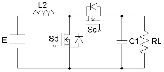
Figure 5.
Mode II converter.
2.3. Mode III (Buck)
The proposed converter can operate bidirectionally with respect to the Mode II. In such scenario, is replaced with a DC power source (e.g., regenerative braking) and the battery E can be charged. In this work, the battery is modeled as a variable-value (bounded) resistance , and the regenerative voltage is considered greater than the battery voltage E; such scenario constitutes a simple charge scenario for lead-acid batteries, and even for other types with a smart charger. The equivalent circuit for this configuration is obtained when , , and are open and and are closed. and are switched alternately integrating a Buck configuration (Figure 6) and the nominal system as obtained in Section 2.1 is:
where , and
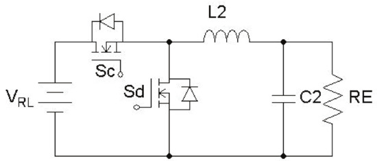
Figure 6.
Mode III converter.
A polytopic system is built similarly to Section 2.1 :
2.4. Mode IV (Buck)
The proposed converter can be used with an additional DC power source () to provide energy to the load using the same Buck converter of Section 2.1; this is, when , , and are open and and are closed the resulting nominal configuration (Figure 7) is described by an analogy to (5) system:
where , and
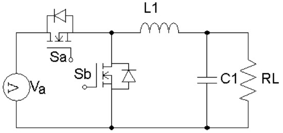
Figure 7.
Mode IV converter.
A polytopic system is built similarly to Section 2.1 :
2.5. Mode V (Cascade Buck)
In Figure 8 is shown the resulting cascade buck converter configuration obtained when and are open and and are closed. The power source is considered of a higher value than the battery voltage E and this mode is used to do a fast-charge of the battery; the battery is modeled as a resistance with variable (bounded) value .
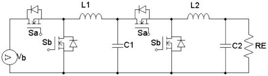
Figure 8.
Mode V converter.
As in Section 2.1, the Mosfets are again modeled as variable resistors with smooth alternate transitions (Figure 9). Voltage in can be calculated as (Figure 10):
and analogously the voltage in :
where is the voltage in .
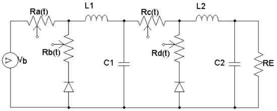
Figure 9.
Idealized mode V converter.
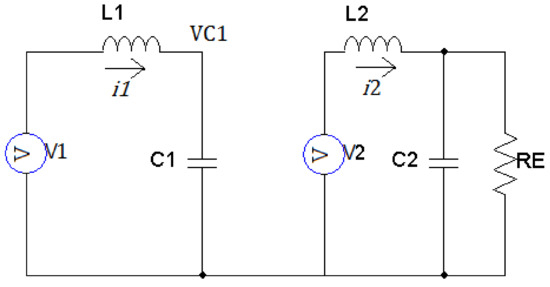
Figure 10.
Idealized mode V converter.
If the Mosfets are considered of the same characteristics and that are activated and deactivated in pairs ( with and with ) then:
where represents the average of the resistances divisor over the time. Equations that describes the dynamic behavior are:
and using the following variable change
the model is equivalently represented by:
Note that the above system is bilinear and in this point it is not possible to build a polytopic system. However, linearization in different operating points is performed for posterior control design and stability study. Multiple linearizations are performed instead of only one in order to describe more accurately the bilinear system. Please consider -dependant linearizations, this is, for the operating point , the resulting linearization is:
where
For the operating point , the resulting linearization is:
where
and successively for n desired linearizations.
A criterion for the recommended number of linearizations is not available in literature; in this work, is proposed to use . This number is obtained by numerical appreciation: when stability margin has no noticeable improvement with respect to the number of linearizations (see Section 3.5).
The obtained system is a switched linear system, and each linearization is then considered as a LPV system and finally as a polytopic system. Therefore the switched polytopic system can be written as:
where denotes the number of the active linearization . Note that is unique for the entire switched polytopic system.
3. Controller Design
In the following, the dynamic models obtained in Section 2 are used to obtain robust control laws for each converter mode and a global stability criterion. In this work, economy and easy implementation are fundamental; a voltage feedback is used in all of the modes. Proportional-Derivative controllers are used in order to provide of flexibility in its behavior in comparison with other control strategies as Sliding Modes ([65]).
3.1. Controller Design for the Mode I (Buck)
The control objective for the design of the Buck controller of Section 2.1 is to design a controller such that stability of the trajectories of the System (7) is ensured for parametric variation within specified design ranges. Consider:
The polytopic system is calculated as:
where the matrix of the nominal system is:
Without loss of generality the origin is considered the equilibrium point, note that a variable change can be performed in order to achieve it. Stability of a polytopic system can be ensured by the following result:
Proposition 1.
[67] Quadratic stability of System (42) is equivalent to the existence of a symmetric, positive definite matrix satisfying:
where denotes a definite negative matrix.
In other words, it is enough to prove that all of the systems built with each vertex (in the following vertex is used to identify a system built with a vertex) are stable using a Common Lyapunov Function (CLF) to ensure that the polytopic system is quadratically stable even under arbitrarily fast parameter variation. Consider the CLF candidate:
with . The time derivative along the trajectories of each vertex has the form:
where if and . Note that the controller gains and can be selected such that for all vertex of the polytopic system. Existence of the CLF allows to conclude that the system trajectories of the polytopic System (42) are quadratically stable for adequate values of and even under arbitrarily fast parameter variation within the design range.
3.2. Controller Design for the Mode II (Boost)
The control objective for the design of the Buck controller of Section 2.2 is to design a controller such that stability of the trajectories of the System (15) is ensured for parametric variation within specified design ranges. Consider:
where with . The polytopic system is calculated as:
where the matrix of the nominal system is:
and the matrix entries of for parametric variation ranges , y is:
Consider any vertex denoted by:
matrix is Hurwitz since determinant of the first minor () is negative and determinant of the second minor () is positive ( and are negative) and existence of a Lyapunov Function is ensured by Theorem 4.6 of [68]. Existence of the CLF allows to conclude that the system trajectories of the polytopic System (15) are quadratically stable for adequate values of and even under arbitrarily fast parameter variation within the design range.
3.3. Controller Design for the Mode III (Buck)
The control objective for the design of the Buck controller of Section 2.3 is to design a controller such that stability of the trajectories of the System (18) is ensured for parametric variation within specified design ranges. As mentioned in Section 2.3, the proposed converter can operate bidirectionally with respect to the Mode II. When is replaced with a regulated DC power source the battery E can be charged; in this work the battery is modeled as a resistance with variable value and the regenerative voltage is considered greater than the battery voltage E. The equivalent circuit for this configuration is obtained when , , and are open and and are closed. and are switched alternately integrating a Buck configuration such that controller design and stability analysis is similar to the proposed in Section 3.1. The resulting controller is:
The polytopic system is calculated as:
where the matrix of the nominal system is:
Existence of the CLF allows to conclude that the system trajectories of the polytopic System (56) are quadratically stable for adequate values of and even under arbitrarily fast parameter variation within the design range.
3.4. Controller Design for the Mode IV (Buck)
The control objective for the design of the Buck controller of Section 2.4 is to design a controller such that stability of the trajectories of the System (21) is ensured for parametric variation within specified design ranges. As mentioned in Section 2.4, the converter can be used with an additional DC power source () to provide energy to the load using the same Buck converter of the Section 2.1; the controller design and stability analysis is similar to the proposed in Section 3.1. The resulting controller is:
where . The polytopic system is calculated as:
where the matrix of the nominal system is:
Existence of the CLF allows to conclude that the system trajectories of the polytopic System (60) are quadratically stable for adequate values of and even under arbitrarily fast parameter variation within the design range, and multiple linearizations.
3.5. Controller Design for the Mode V (Cascade Buck)
The control objective for the design of the Buck controller of Section 2.5 is to design a controller such that stability of the trajectories of the System (40) is ensured for parametric variation within specified design ranges. Stability of the switched polytopic system can be ensured using the Theorem 1 proposed in [69] and is equivalent to find a CLF for every vertex of every linearization. Consider:
It follows that the closed loop system for some vertex of some linearization is:
Consider the Lyapunov candidate , the time derivative along trajectories of the system is:
3.6. Global Stability
In this section, the global stability of , for the switching between all the forward load supply modes is studied; Some considerations are performed to this end as follows.
Since Mode V is designed for a fast, and off-line battery recharge, a slow switching dynamic can be considered (the delay to change to this mode is considerably larger than the switching between the other online modes) allowing to decouple its dynamics from the global switching stability considerably simplifying the analysis.
The switching between the Mode III and any other mode, in a real implementation scenario, must be performed considering the discharge of in order to avoid current peaks that the electric/electronic components possibly cannot support.
In order to show the global stability, first a similar structure for all the modes is proposed and second it is proposed a CLF that ensures the result. Consider any vertex of the Mode 1, substituting (3) in (4):
Using (41):
With a variable change :
and using a CLF candidate
with , follows that time derivative along trajectories system:
if:
and
Substituting (76) in (77) the stability conditions, in congruence with those of Section 3.1 are:
where is a real number .
For any vertex of the Mode II it is possible to use the same (74) CLF structure and the resulting stability conditions are:
where is a real number .
For any vertex of the Mode III, turns in a power source with voltage such that stability of voltage is guaranteed with the same (74) CLF.
For any vertex of the Mode IV it is possible to use the same (74) CLF structure and the resulting stability conditions are:
where is a real number .
The previous stability conditions for all of the modes, allows to perform an integration of all conditions in a single condition for each controller gain:
and if the following conditions are accomplished
where i stands for the vertex, stands for the mode constant, stands for referring to an inductor and stands for the source voltage. Note that under the aforementioned conditions, the stability on output voltage is ensured even under fast parameter variation; however, the switch from Mode III to Modes II/V (and vice versa) must be performed considering the discharge of in order to avoid current peaks.
4. Simulations
In this section, representative simulations for the modes is presented. Simulations are performed in Simulink with a switching frequency of 50 kHz and an integration time of 100 ns. Maximum duty cycle is established in 85% and nominal values are , mH, F with variation ranges for controller design of . In Figure 11 is shown a comparative of the output voltage against a fast change in the value of , with a setpoint of ten volts, in 3 cases: open loop, using a sliding modes controller, and with the proposed controller. A comparative for the voltage in Mode I (buck), the load resistance is alternated to 40 every 10 ms and the output voltage is compared open loop vs. sliding modes vs. present robust PD controller. Note that robust PD allows to modify controller gains in order to obtain a response without overshoot. In Figure 12 is shown simulation data for the in Mode II controller (boost), with changes on set point and load; again, the robust PD response avoids the overshoot. In Figure 13 is shown simulation data for the in Mode V controller (cascade buck), the load resistance is alternated to 40 every 10 ms and the output voltage is compared open loop vs sliding modes vs present robust PD controller. Note that robust PD allows to modify controller gains in order to obtain a response without overshoot.
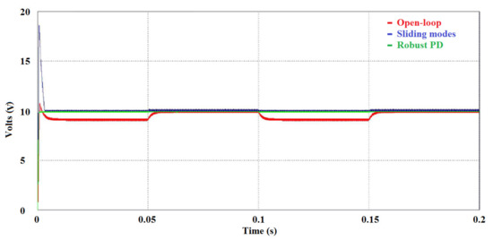
Figure 11.
Mode I control comparative.
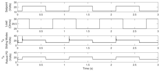
Figure 12.
Mode II control comparative.
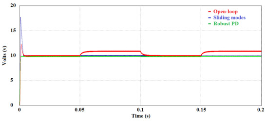
Figure 13.
Mode V control comparative.
5. Experimental Behavior
In order to illustrate the functioning of the control, experiments are performed with the schematic shown in Figure 1 implemented with low-cost components, a MICROCHIP dsPICDEM Plus board, an interface circuit, power supplies and an electronic load. The resulting PCB is illustrated in Figure 14. The dsPICDEM has a DsPIC30F6014 chip running at 29,400 MIPS; this chip is a low-cost DSP (about USD) and it can operate with a minimum of external components since oscillator is integrated on-chip, only a voltage regulator and a couple of capacitors are required for reducing this stage (for production purposes).
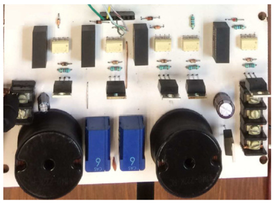
Figure 14.
Printed Circuit Board of the converter with activation circuit.
For the experiments, two representative modes with their respective tests were selected. For the former test, Mode II (Boost) is used with a 50 V input voltage E while the reference is set to 55 V. The controller gains are manually tuned ever selected to accomplish with the Conditions (86) and (87). Abrupt resistance value modifications are performed starting with 200 to 3 and to 100 reaching consumption peaks of 400 W. In Figure 15 and Figure 16 are shown the oscilloscope and electronic load captures respectively; ripple is higher when the load decreases as expected but note that the average voltage suffers only a 2 V drop and that there are no undesirable effects, even while load value changes.
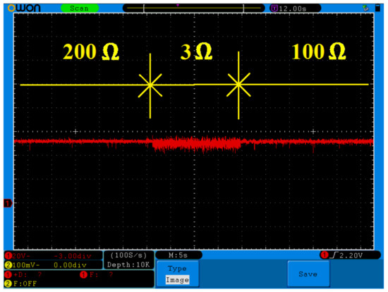
Figure 15.
Mode II closed loop response against abrupt load changes.
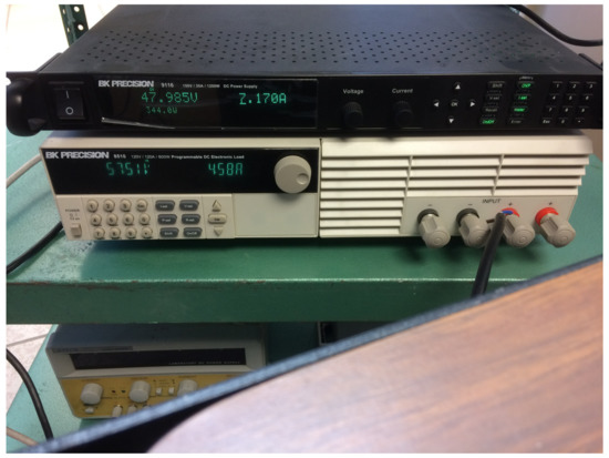
Figure 16.
Main power supply and electronic load in Mode II with load.
In the later test, Mode I (Buck) is used with a 24 V input voltage E while the reference is set to 10 V. Under similar test conditions, the voltage drop is about 2 V as illustrated in Figure 17.
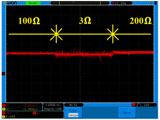
Figure 17.
Mode I closed loop response against abrupt load changes.
6. Conclusions
In the present work, a reconfigurable DC-DC converter with a Polytopic/Robust PD controller design is presented. This bidirectional converter can be used in EV applications as a single solution to power distribution since includes a special battery recharge mode for regenerative charging and also for high voltage charging mode for a fast recharge.
In comparison with other control schemes, the controller gains can be adjusted and a stability of output voltage analysis is presented in order to claim a quantifiable robust behavior in face of parametric uncertainty and abrupt set point/load changes. Further, the stability of the output voltage between modes switching is also presented and implementation of the control can be analog or digital and of low cost. An experimental testbed is presented in order to illustrate the controller performance.
The main objective of this paper is to establish the low-level stability to the setpoint and the stability between the switching of modes; in such scenario, a higher level supervisor with an optimal energy management algorithm must be capable of sending appropriate commands and the design of such supervisor is out of the scope of this paper. As a future work, a higher level supervisor that order the levels of setpoint and the module that must be active at a specific time, for an EV case will be presented.
Author Contributions
Martin-A. Rodríguez-Licea conceived and designed the experiments; Martin-A. Rodríguez-Licea performed the experiments; Martin-A. Rodríguez-Licea, Francisco-J. Pérez-Pinal, Alejandro-I. Barranco-Gutiérrez and Jose-C. Nuñez-Perez analyzed the data; Martin-A. Rodríguez-Licea, Francisco-J. Pérez-Pinal, Alejandro-I. Barranco-Gutiérrez and Jose-C. Nuñez-Perez contributed materials/analysis tools; Martin-A. Rodríguez-Licea and Francisco-J. Pérez-Pinal wrote the paper.
Conflicts of Interest
The authors declare no conflict of interest for this paper.
Abbreviations
The following abbreviations are used in this manuscript:
| CLF | Common Lyapunov function |
| DC | Direct Current |
| HPS | High-pressure sodium |
| IoT | Internet of things |
| LED | Light Emitting Diode |
| LPV | Linear Parameter Variant |
| PEC | Power electronic converters |
| PSS | Polytopic Switched System |
| RE | Renewable energy |
| RLC | Resistance-Inductor-Capacitor |
| RPEC | Reconfigurable power electronic converters |
| SLPV | Switched linear parameter varying |
| SPC | Switched polytopic controller |
| TE | Transport electrification |
References
- Erickson, R.W.; Maksimovic, D. Fundamentals of Power Electronics; Springer Science & Business Media: Berlin, Germany, 2007. [Google Scholar]
- Ang, S.; Oliva, A. Power-Switching Converters; CRC Press: Boca Raton, FL, USA, 2005. [Google Scholar]
- Lee, S.W.; Do, H.L. Boost Integrated Two-Switch Forward AC-DC LED Driver with High Power Factor and Ripple-Free Output Inductor Current. IEEE Trans. Ind. Electron. 2017, 64, 5789–5796. [Google Scholar] [CrossRef]
- Cheng, H.L.; Cheng, C.A.; Chang, Y.N.; Tsai, K.M. Analysis and implementation of an integrated electronic ballast for high-intensity-discharge lamps featuring high-power factor. IET Power Electron. 2013, 6, 1010–1018. [Google Scholar] [CrossRef]
- Alonso, J.M.; Viña, J.; Vaquero, D.G.; Martínez, G.; Osorio, R. Analysis and design of the integrated double buck–boost converter as a high-power-factor driver for power-LED lamps. IEEE Trans. Ind. Electron. 2012, 59, 1689–1697. [Google Scholar] [CrossRef]
- Dalla Costa, M.A.; Marchesan, T.B.; da Silveira, J.S.; Seidel, Á.R.; do Prado, R.N.; Álvarez, J.M.A. Integrated power topologies to supply HPS lamps: A comparative study. IEEE Trans. Power Electron. 2010, 25, 2124–2132. [Google Scholar] [CrossRef]
- Kim, D.H.; Kim, M.J.; Lee, B.K. An Integrated Battery Charger With High Power Density and Efficiency for Electric Vehicles. IEEE Trans. Power Electron. 2017, 32, 4553–4565. [Google Scholar] [CrossRef]
- Ashique, R.H.; Salam, Z.; Aziz, M.J.B.A.; Bhatti, A.R. Integrated photovoltaic-grid dc fast charging system for electric vehicle: A review of the architecture and control. Renew. Sustain. Energy Rev. 2017, 69, 1243–1257. [Google Scholar] [CrossRef]
- Ebrahimi, S.; Akbari, R.; Tahami, F.; Oraee, H. An Isolated Bidirectional Integrated Plug-in Hybrid Electric Vehicle Battery Charger with Resonant Converters. Electr. Power Compon. Syst. 2016, 44, 1371–1383. [Google Scholar] [CrossRef]
- Dusmez, S.; Khaligh, A. A compact and integrated multifunctional power electronic interface for plug-in electric vehicles. IEEE Trans. Power Electron. 2013, 28, 5690–5701. [Google Scholar] [CrossRef]
- Hegazy, O.; Barrero, R.; Van Mierlo, J.; Lataire, P.; Omar, N.; Coosemans, T. An advanced power electronics interface for electric vehicles applications. IEEE Trans. Power Electron. 2013, 28, 5508–5521. [Google Scholar] [CrossRef]
- Saponara, S.; Tisserand, P.; Chassard, P.; Ton, D.M. Design and Measurement of Integrated Converters for Belt-Driven Starter-Generator in 48 V Micro/Mild Hybrid Vehicles. IEEE Trans. Ind. Appl. 2017, 53, 3936–3949. [Google Scholar] [CrossRef]
- Uno, M.; Kukita, A. PWM converter integrating switched capacitor converter and series-resonant voltage multiplier as equalizers for photovoltaic modules and series-connected energy storage cells for exploration rovers. IEEE Trans. Power Electron. 2017, 32, 8500–8513. [Google Scholar] [CrossRef]
- Chen, G.; Deng, Y.; Wang, K.; Hu, Y.; Jiang, L.; Wen, H.; He, X. Topology Derivation and Analysis of Integrated Multiple Output Isolated DC-DC Converters with Stacked Configuration for Low-Cost Applications. IEEE Trans. Circuits Syst. I Regul. Pap. 2017, 64, 2207–2218. [Google Scholar] [CrossRef]
- Sulligoi, G.; Vicenzutti, A.; Arcidiacono, V.; Khersonsky, Y. Voltage stability in large marine-integrated electrical and electronic power systems. IEEE Trans. Ind. Appl. 2016, 52, 3584–3594. [Google Scholar] [CrossRef]
- Pan, L.; Zhang, C. An Integrated Multifunctional Bidirectional AC/DC and DC/DC Converter for Electric Vehicles Applications. Energies 2016, 9, 493. [Google Scholar] [CrossRef]
- McCoy, T.J. Integrated power systems—An outline of requirements and functionalities for ships. Proc. IEEE 2015, 103, 2276–2284. [Google Scholar] [CrossRef]
- Kim, S.Y.; Choe, S.; Ko, S.; Sul, S.K. A Naval Integrated Power System with a Battery Energy Storage System: Fuel efficiency, reliability, and quality of power. IEEE Electr. Mag. 2015, 3, 22–33. [Google Scholar] [CrossRef]
- Hsieh, C.Y.; Moallem, M.; Golnaraghi, F. A Bidirectional Boost Converter With Application to a Regenerative Suspension System. IEEE Trans. Veh. Technol. 2016, 65, 4301–4311. [Google Scholar] [CrossRef]
- Abebe, R.; Vakil, G.; Calzo, G.L.; Cox, T.; Lambert, S.; Johnson, M.; Gerada, C.; Mecrow, B. Integrated motor drives: State of the art and future trends. IET Electr. Power Appl. 2016, 10, 757–771. [Google Scholar] [CrossRef]
- Sulligoi, G.; Vicenzutti, A.; Menis, R. All-Electric Ship Design: From Electrical Propulsion to Integrated Electrical and Electronic Power Systems. IEEE Trans. Transp. Electr. 2016, 2, 507–521. [Google Scholar] [CrossRef]
- Emadi, A.; Williamson, S.S.; Khaligh, A. Power electronics intensive solutions for advanced electric, hybrid electric, and fuel cell vehicular power systems. IEEE Trans. Power Electron. 2006, 21, 567–577. [Google Scholar] [CrossRef]
- Leuenberger, D.; Biela, J. PV-Module-Integrated AC Inverters (AC Modules) with Subpanel MPP Tracking. IEEE Trans. Power Electron. 2017, 32, 6105–6118. [Google Scholar] [CrossRef]
- Zhong, Q.C.; Blaabjerg, F.; Cecati, C. Power-Electronics-Enabled Autonomous Power Systems. IEEE Trans. Ind. Electron. 2017, 64, 5904–5906. [Google Scholar] [CrossRef]
- Chub, A.; Vinnikov, D.; Kosenko, R.; Liivik, E. Wide Input Voltage Range Photovoltaic Microconverter with Reconfigurable Buck–Boost Switching Stage. IEEE Trans. Ind. Electron. 2017, 64, 5974–5983. [Google Scholar] [CrossRef]
- Chatterjee, A.; Mohanty, K.; Kommukuri, V.S.; Thakre, K. Design and experimental investigation of digital model predictive current controller for single phase grid integrated photovoltaic systems. Renew. Energy 2017, 108, 438–448. [Google Scholar] [CrossRef]
- Li, F.; Liu, H. A Cascaded Coupled Inductor-Reverse High Step-Up Converter Integrating Three-Winding Coupled Inductor and Diode–Capacitor Technique. IEEE Trans. Ind. Inform. 2017, 13, 1121–1130. [Google Scholar] [CrossRef]
- Zhang, N.; Sutanto, D.; Muttaqi, K.M. A review of topologies of three-port DC-DC converters for the integration of renewable energy and energy storage system. Renew. Sustain. Energy Rev. 2016, 56, 388–401. [Google Scholar] [CrossRef]
- Verma, A.K.; Singh, B.; Shahani, D.T.; Jain, C. Grid-interfaced Solar Photovoltaic Smart Building with Bidirectional Power Flow Between Grid and Electric Vehicle with Improved Power Quality. Electr. Power Compon. Syst. 2016, 44, 480–494. [Google Scholar] [CrossRef]
- Maity, S.; Sahu, P.K. Modeling and analysis of a fast and robust module-integrated analog photovoltaic MPP tracker. IEEE Trans. Power Electron. 2016, 31, 280–291. [Google Scholar] [CrossRef]
- Li, Y.R.; Hurley, W.G. Editorial Special Issue on Sustainable Energy Systems Integration. IEEE J. Emerg. Sel. Top. Power Electron. 2015, 3, 854–857. [Google Scholar] [CrossRef]
- Novakovic, B.; Nasiri, A. Modular Multilevel Converter for Wind Energy Storage Applications. IEEE Trans. Ind. Electron. 2017, 64, 8867–8876. [Google Scholar] [CrossRef]
- Li, Y.; Han, Y. A module-integrated distributed battery energy storage and management system. IEEE Trans. Power Electron. 2016, 31, 8260–8270. [Google Scholar] [CrossRef]
- Dusmez, S.; Li, X.; Akin, B. A new multiinput three-level DC/DC converter. IEEE Trans. Power Electron. 2016, 31, 1230–1240. [Google Scholar] [CrossRef]
- Aguilar, C.; Vazquez, A.; Canales, F.; Gordillo, J. Integrated DC-AC Converter as Power Conditioner for Fuel Cell Based System. IEEE Lat. Am. Trans. 2016, 14, 2107–2113. [Google Scholar] [CrossRef]
- Adly, M.; Strunz, K. Irradiance-adaptive PV Module Integrated Converter for High Efficiency and Power Quality in Standalone and DC Microgrid Applications. IEEE Trans. Ind. Electron. 2017, 65, 436–446. [Google Scholar] [CrossRef]
- Siwakoti, Y.P.; Blaabjerg, F. Single Switch Nonisolated Ultra-Step-Up DC-DC Converter with an Integrated Coupled Inductor for High Boost Applications. IEEE Trans. Power Electron. 2017, 32, 8544–8558. [Google Scholar] [CrossRef]
- Cecati, C.; Khalid, H.A.; Tinari, M.; Adinolfi, G.; Graditi, G. DC nanogrid for renewable sources with modular DC/DC LLC converter building block. IET Power Electron. 2016, 10, 536–544. [Google Scholar] [CrossRef]
- Qin, S.; Barth, C.B.; Pilawa-Podgurski, R.C. Enhancing microinverter energy capture with submodule differential power processing. IEEE Trans. Power Electron. 2016, 31, 3575–3585. [Google Scholar] [CrossRef]
- Strunz, K.; Abbasi, E.; Huu, D.N. DC microgrid for wind and solar power integration. IEEE J. Emerg. Sel. Top. Power Electron. 2014, 2, 115–126. [Google Scholar] [CrossRef]
- Gutierrez, F. Fully-Integrated Converter for Low-Cost and Low-Size Power Supply in Internet-of-Things Applications. Electronics 2017, 6, 38. [Google Scholar] [CrossRef]
- Almer, S.; Fujioka, H.; Jonsson, U.; Kao, C.Y.; Patino, D.; Riedinger, P.; Geyer, T.; Beccuti, A.; Papafotiou, G.; Morari, M.; et al. Hybrid control techniques for switched-mode DC-DC converters Part I: The step-down topology. In Proceedings of the American Control Conference, New York, NY, USA, 9–13 July 2007; IEEE: Piscataway, NJ, USA, 2007; pp. 5450–5457. [Google Scholar]
- Orłowska-Kowalska, T.; Blaabjerg, F.; Rodríguez, J. Advanced and Intelligent Control in Power Electronics and Drives; Springer: Berlin/Heidelberg, Germany, 2014; Volume 531. [Google Scholar]
- Vlad, C.; Rodriguez-Ayerbe, P.; Godoy, E.; Lefranc, P. Advanced control laws of DC-DC converters based on piecewise affine modelling. Application to a step-down converter. IET Power Electron. 2014, 7, 1482–1498. [Google Scholar] [CrossRef]
- Zeng, J.; Zhang, Z.; Qiao, W. An interconnection and damping assignment passivity-based controller for a DC-DC boost converter with a constant power load. IEEE Trans. Ind. Appl. 2014, 50, 2314–2322. [Google Scholar] [CrossRef]
- Khaligh, A.; Rahimi, A.M.; Emadi, A. Modified pulse-adjustment technique to control DC/DC converters driving variable constant-power loads. IEEE Trans. Ind. Electron. 2008, 55, 1133–1146. [Google Scholar] [CrossRef]
- Cervantes, I.; Perez-Pinal, F.J.; Mendoza-Torres, A. Hybrid Control of DC-DC power converters. In Renewable Energy; InTech: Chattanooga, TN, USA, 2009. [Google Scholar]
- Johansen, T.A.; De Molengraft, R.; Nijmeijer, H. Switched, piecewise and polytopic linear systems. Int. J. Control 2002, 75, 1241–1242. [Google Scholar] [CrossRef]
- Bengea, S.; DeCarlo, R.; Corless, M.; Rizzoni, G.; Yurkovich, S. A Polytopic System Approach for Gain Scheduled Control of a Diesel Engine. IFAC Proc. Vol. 2002, 35, 349–354. [Google Scholar] [CrossRef]
- Andrade-Da Silva, J.M.; Edwards, C.; Spurgeon, S.K. Sliding-mode output-feedback control based on LMIs for plants with mismatched uncertainties. IEEE Trans. Ind. Electron. 2009, 56, 3675–3683. [Google Scholar] [CrossRef]
- Donkers, M.; Heemels, W.; Van de Wouw, N.; Hetel, L. Stability analysis of networked control systems using a switched linear systems approach. IEEE Trans. Autom. Control 2011, 56, 2101–2115. [Google Scholar] [CrossRef]
- Huang, Y.; Changyin, Q.; Chengshan, Z.; Jingmei, W. Polytopic LPV modeling and gain-scheduled switching control for a flexible air-breathing hypersonic vehicle. J. Syst. Eng. Electron. 2013, 2, 118–127. [Google Scholar] [CrossRef]
- Wang, Z.; Wang, Q.; Dong, C. Asynchronous H infinite control for unmanned aerial vehicles: Switched polytopic system approach. IEEE/CAA J. Autom. Sin. 2015, 2, 207–216. [Google Scholar]
- Yang, T.; Li, A.; Niu, E. Robust dynamic output feedback control for switched polytopic systems under asynchronous switching. Chin. J. Aeronaut. 2015, 28, 1226–1235. [Google Scholar] [CrossRef]
- Dong, C.; Ma, A.; Wang, Q.; Wang, Z. Robust fault-tolerant tracking control for nonlinear networked control system: Asynchronous switched polytopic approach. Math. Probl. Eng. 2015, 2015, 903058. [Google Scholar] [CrossRef]
- Zhang, L.; Wang, S.; Karimi, H.R.; Jasra, A. Robust finite-time control of switched linear systems and application to a class of servomechanism systems. IEEE/ASME Trans. Mechatron. 2015, 20, 2476–2485. [Google Scholar] [CrossRef]
- Liu, Y.; Yang, J.; Li, C. Robust finite-time stability and stabilisation for switched linear parameter-varying systems and its application to bank-to-turn missiles. IET Control Theory Appl. 2015, 9, 2171–2179. [Google Scholar] [CrossRef]
- Liu, J.; Zhang, K.; Pang, G.; Wei, H. Robust stabilisation for constrained discrete-time switched positive linear systems with uncertainties. IET Control Theory Appl. 2015, 9, 2598–2605. [Google Scholar] [CrossRef]
- Glover, S.F. Modeling and Stability Analysis of a Power Electronics Based Systems. Ph.D. Thesis, Department of Electrical Engineering, Purdue University, Lafayette, IN, USA, 2003. [Google Scholar]
- Arnedo, L.; Boroyevich, D.; Burgos, R.; Wang, F. Polytopic black-box modeling of DC-DC converters. In Proceedings of the Power Electronics Specialists Conference, Rhodes, Greece, 15–19 June 2008; IEEE: Piscataway, NJ, USA, 2008; pp. 1015–1021. [Google Scholar]
- Francés, A.; Asensi, R.; García, O.; Uceda, J. A blackbox large signal Lyapunov-based stability analysis method for power converter-based systems. In Proceedings of the 2016 IEEE 17th Workshop on Control and Modeling for Power Electronics (COMPEL), Trondheim, Norway, 27–30 June 2016; IEEE: Piscataway, NJ, USA, 2016; pp. 1–6. [Google Scholar]
- Francés, A.; Asensi, R.; García, O.; Prieto, R.; Uceda, J. A black-box modeling approach for DC nanogrids. In Proceedings of the 2016 IEEE Applied Power Electronics Conference and Exposition (APEC), Long Beach, CA, USA, 20–24 March 2016; IEEE: Piscataway, NJ, USA, 2016; pp. 1624–1631. [Google Scholar]
- Francés, A.; Asensi, R.; García, O.; Prieto, R.; Uceda, J. The performance of polytopic models in smart DC microgrids. In Proceedings of the 2016 IEEE Energy Conversion Congress and Exposition (ECCE), Milwaukee, WI, USA, 18–22 September 2016; IEEE: Piscataway, NJ, USA, 2016; pp. 1–8. [Google Scholar]
- Aguilar-Najar, R.; Perez-Pinal, F.J.; Herrera-Ramirez, C.; Barranco-Gutiérrez, A. Novel positive integrated converter. In Proceedings of the 2016 13th International Conference on Power Electronics (CIEP), Guanajuato, Mexico, 20–23 June 2016; IEEE: Piscataway, NJ, USA, 2016; pp. 41–46. [Google Scholar]
- Sira-Ramírez, H.; Silva-Ortigoza, R. Control Design Techniques in Power Electronics Devices; Springer Science & Business Media: Berlin, Germany, 2006. [Google Scholar]
- Nehrir, M.H.; Wang, C. Modeling and Control of Fuel Cells: Distributed Generation Applications; John Wiley & Sons: Hoboken, NJ, USA, 2009; Volume 41. [Google Scholar]
- Boyd, S.; El Ghaoui, L.; Feron, E.; Balakrishnan, V. Linear Matrix Inequalities in System and Control Theory; SIAM: Philadelphia, PA, USA, 1994. [Google Scholar]
- Khalil, H.K. Noninear Systems; Prentice-Hall: Upper Saddle River, NJ, USA, 1996. [Google Scholar]
- Licea, M.R.; Cervantes, I. Robust indirect-defined envelope control for rollover and lateral skid prevention. Control Eng. Pract. 2017, 61, 149–162. [Google Scholar] [CrossRef]
© 2018 by the authors. Licensee MDPI, Basel, Switzerland. This article is an open access article distributed under the terms and conditions of the Creative Commons Attribution (CC BY) license (http://creativecommons.org/licenses/by/4.0/).