Real-Power Rescheduling of Generators for Congestion Management Using a Novel Satin Bowerbird Optimization Algorithm

Abstract
:1. Introduction
1.1. Inspiration of SBO
- (a)
- SBO provides competitive or slightly better performance compared with other bio-inspired algorithms in a stand test function;
- (b)
- SBO has good exploitation capabilities, which optimize the solution through small and reasonable changes in variables;
- (c)
- SBO performs with real-world data sets, unlike other bio-inspired algorithms; and
- (d)
- SBO focuses on the best solution while constantly searching for new solutions in the search space.
1.2. Objective of the Present Work
- (a)
- SBO algorithm tool effectively minimizes the changing generator real-power rescheduling cost;
- (b)
- Effectively relieves the congestion in overloaded lines with different contingency cases; and
- (c)
- Minimizes the losses indifferent contingencies of the test system cases.
2. Mathematical Problem Formulation
2.1. Equality Constraints
2.2. Inequality Constraints
3. Satin Bowerbird Optimization (SBO)
3.1. Introduction of SBO
3.2. SBO Algorithm
3.2.1. Generating a Set of Random Bowers
3.2.2. Calculating the Probability of Each Population Member
3.2.3. Elitism
3.2.4. Determining New Changes in Any Position
3.2.5. Mutation
3.2.6. Combining the Old Population and the Population Obtained from Changes
3.3. Pseudocode for SBO Algorithm
| Algorithm |
| Initialize the first population of bowers randomly |
| Calculate the cost of bowers |
| Find the best bower and assume it as elite |
 |
| Return best bower |
4. Proposed SBO Algorithm for CM Application
Computational Procedure for SBO Algorithm for CM
5. Simulation Results and Discussion
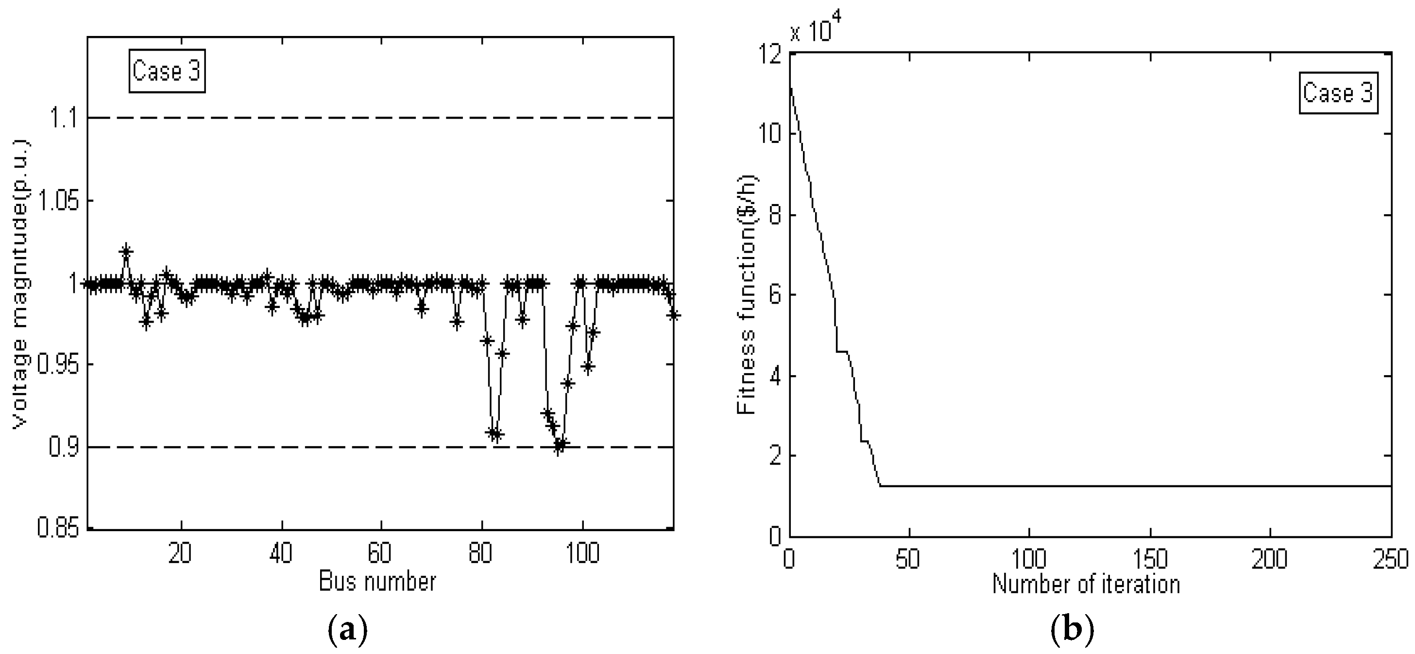
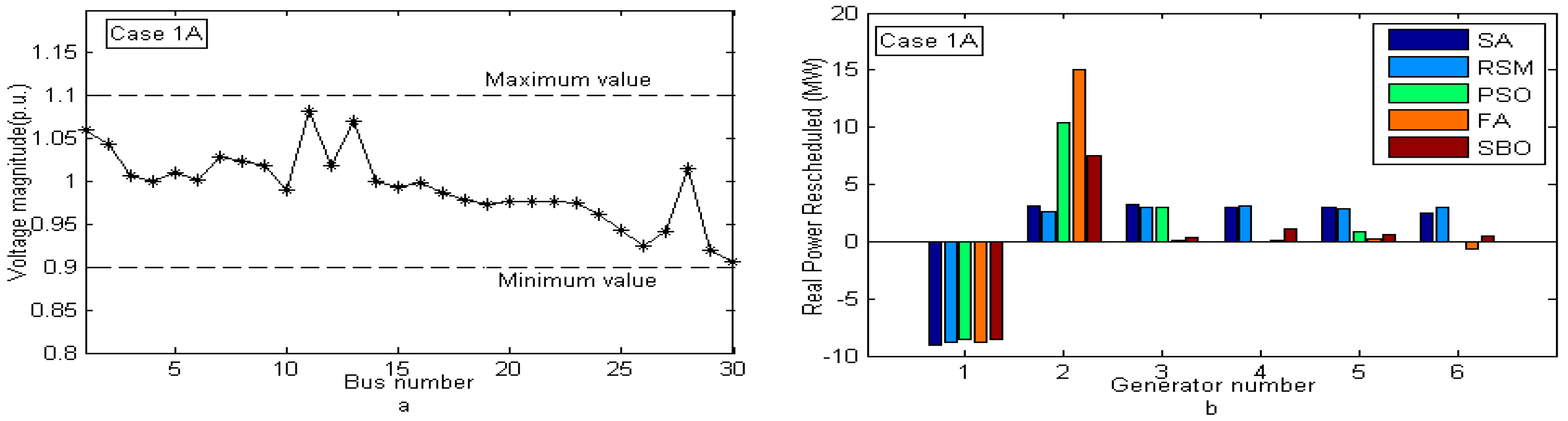
5.1. Modified IEEE 30-Bus Test System
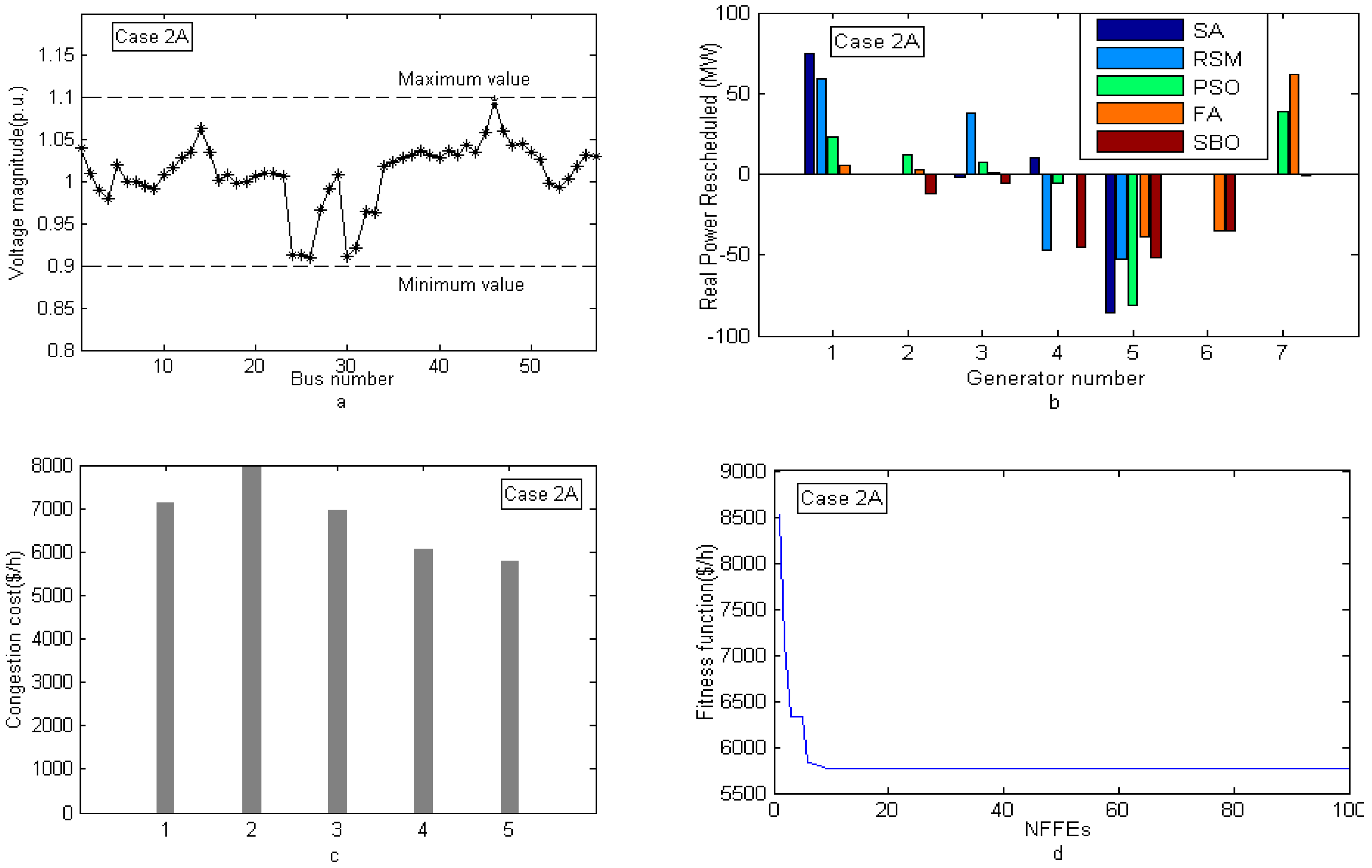
5.2. Modified IEEE 57-Bus Test System
5.3. IEEE 118-Bus Test System
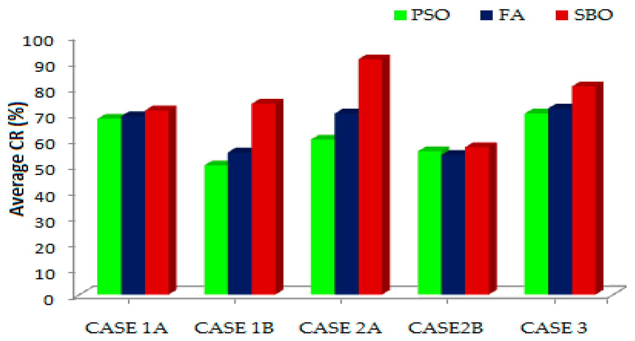
6. Convergence Mobility and Effectiveness of SBO
- (a)
- Run the algorithms up to the maximum of NFFE (number of fitness function evaluation) (NFFEmax);
- (b)
- Based on convergence, determine NFFER, which is the NFFE corresponding to the minimum objective value; and
- (c)
- Compute the CR for the algorithm by using Equation (21).
7. Conclusions
Acknowledgments
Author Contributions
Conflicts of Interest
Appendix A

| Bus Number | Increment (CtG), $/MWh | Decrement (DtG), $/MWh | Bus Number | Increment (CtG), $/MWh | Decrement (DtG,) $/MWh |
|---|---|---|---|---|---|
| Modified IEEE 30-bus test system [7] | |||||
| 1 | 22 | 18 | 4 | 43 | 37 |
| 2 | 21 | 19 | 5 | 43 | 35 |
| 3 | 42 | 38 | 6 | 41 | 39 |
| Modified IEEE 57-bus test system [7] | |||||
| 1 | 44 | 41 | 5 | 42 | 39 |
| 2 | 43 | 39 | 6 | 44 | 40 |
| 3 | 42 | 38 | 7 | 44 | 41 |
| 4 | 43 | 37 | |||
| IEEE 118-bus test system [19] | |||||
| 1 | 40 | 38 | 65 | 25 | 17 |
| 4 | 43 | 35 | 66 | 26 | 18 |
| 6 | 41 | 38 | 69 | 28 | 15 |
| 8 | 44 | 39 | 70 | 43 | 39 |
| 10 | 22 | 17 | 72 | 47 | 38 |
| 12 | 23 | 18 | 73 | 44 | 36 |
| 15 | 45 | 35 | 74 | 43 | 39 |
| 18 | 41 | 38 | 76 | 44 | 36 |
| 19 | 44 | 36 | 77 | 47 | 38 |
| 24 | 45 | 35 | 80 | 23 | 15 |
| 25 | 27 | 18 | 85 | 43 | 39 |
| 26 | 23 | 18 | 87 | 25 | 17 |
| 27 | 41 | 39 | 89 | 44 | 36 |
| 31 | 45 | 35 | 90 | 42 | 38 |
| 32 | 24 | 18 | 91 | 41 | 38 |
| 34 | 43 | 37 | 92 | 44 | 36 |
| 36 | 44 | 36 | 99 | 43 | 37 |
| 40 | 43 | 35 | 100 | 42 | 36 |
| 42 | 47 | 38 | 103 | 24 | 17 |
| 46 | 45 | 35 | 104 | 44 | 38 |
| 49 | 25 | 18 | 105 | 43 | 39 |
| 54 | 32 | 30 | 107 | 42 | 38 |
| 55 | 42 | 36 | 110 | 43 | 37 |
| 56 | 43 | 37 | 111 | 22 | 18 |
| 59 | 23 | 17 | 112 | 42 | 38 |
| 61 | 26 | 16 | 113 | 47 | 33 |
| 62 | 44 | 36 | 116 | 45 | 35 |
References
- Lai, L.L. Energy Generation under the New Environment. In Power System Restructuring and Deregulation; John Wiley & Sons, Ltd.: Hoboken, NJ, USA, 2001; pp. 1–49. ISBN 9780470846117. [Google Scholar]
- Kumar, A.; Srivastava, S.C.; Singh, S.N. Congestion management in competitive power market: A bibliographical survey. Electr. Power Syst. Res. 2005, 76, 153–164. [Google Scholar] [CrossRef]
- Pillay, A.; Prabhakar Karthikeyan, S.; Kothari, D.P. Congestion management in power systems—A review. Int. J. Electr. Power Energy Syst. 2015, 70, 83–90. [Google Scholar] [CrossRef]
- Christie, R.D.; Wollenberg, B.F.; Wangensteen, I. Transmission management in the deregulated environment. Proc. IEEE 2000, 88, 170–195. [Google Scholar] [CrossRef]
- Bombard, E.; Correia, P.; Gross, G.; Amelin, M. Congestion management schemes: A comparative analysis under a unified framework. IEEE Trans. Power Syst. 2003, 18, 346–352. [Google Scholar] [CrossRef]
- Alomoush, M.I.; Shahidehpour, S.M. Contingency-constrained congestion management with a minimum number of adjustments in preferred schedules. Int. J. Electr. Power Energy Syst. 2000, 22, 277–290. [Google Scholar] [CrossRef]
- Chintam, J.R.; Mary, D.; Thanigaimani, P.; Salomipuspharaj, P. A zonal congestion management using hybrid evolutionary firefly (HEFA) algorithm. Int. J. Appl. Eng. Res. 2015, 10, 39903–39910. [Google Scholar]
- Kumar, A.; Mittapalli, R.K. Congestion management with generic load model in hybrid electricity markets with FACTS devices. Int. J. Electr. Power Energy Syst. 2014, 57, 49–63. [Google Scholar] [CrossRef]
- Sujatha Balaraman, N.K. Transmission Congestion Management Using Particle Swarm Optimization. J. Electr. Syst. 2011, 7, 54–70. [Google Scholar]
- Jang, J.S.R.; Sun, C A.T.; Mizutani, E. Neuro-Fuzzy nd Soft Computing—A Computational Approach to Learning and Machine Intelligence. IEEE Trans. Autom. Control 1997, 42, 1482–1484. [Google Scholar] [CrossRef]
- Kumar, A.; Sekhar, C. Congestion management with FACTS devices in deregulated electricity markets ensuring loadability limit. Int. J. Electr. Power Energy Syst. 2013, 46, 258–273. [Google Scholar] [CrossRef]
- Balaraman, S.; Kamaraj, N. Congestion management in deregulated power system using real coded genetic algorithm. Int. J. Eng. Sci. Technol. 2010, 2, 6681–6690. [Google Scholar]
- Yang, X.S. Engineering Optimization: An Introduction with Metaheuristic Applications; John Wiley & Sons, Ltd.: Hoboken, NJ, USA, 2010; ISBN 9780470582466. [Google Scholar]
- Yang, X.-S. Firefly Algorithm, Stochastic Test Functions and Design Optimisation. Int. J. Bio-Inspired Comput. 2010, 2, 78–84. [Google Scholar] [CrossRef]
- Yang, X.-S.; Karamanoglu, M.; He, X.S. Flower Pollination Algorithm: A Novel Approach for Multiobjective Optimization. Eng. Optim. 2014, 46, 1222–1237. [Google Scholar] [CrossRef]
- Yang, X.-S. Bat algorithm for multi-objective optimisation. Int. J. Bio-Inspired Comput. 2011, 3, 267–274. [Google Scholar] [CrossRef]
- Cheng, M.Y.; Prayogo, D. Symbiotic Organisms Search: A new metaheuristic optimization algorithm. Comput. Struct. 2014, 139, 98–112. [Google Scholar] [CrossRef]
- Kothari, D.P. Power Syem Optimisations; PHI: New Delhi, India, 2010. [Google Scholar]
- Samareh Moosavi, S.H.; Khatibi Bardsiri, V. Satin bowerbird optimizer: A new optimization algorithm to optimize ANFIS for software development effort estimation. Eng. Appl. Artif. Intell. 2017, 60, 1–15. [Google Scholar] [CrossRef]
- Coleman, S.W.; Patricelli, G.L.; Borgia, G. Variable female preferences drive complex male displays. Nature 2004, 428, 742–745. [Google Scholar] [CrossRef] [PubMed]
- Borgia, G. Bower destruction and sexual competition in the satin bowerbird (Ptilonorhynchus violaceus). Behav. Ecol. Sociobiol. 1985, 18, 91–100. [Google Scholar] [CrossRef]
- Balaraman, S. Applications of Evolutionary Algorithms and Neural Network for Congestion Management in Power Systems; Anna University: Chennai, India, 2011. [Google Scholar]
- Verma, S.; Mukherjee, V. Firefly algorithm for congestion management in deregulated environment. Eng. Sci. Technol. Int. J. 2016, 19, 1254–1265. [Google Scholar] [CrossRef]
- Gandomi, A.H. Interior search algorithm (ISA): A novel approach for global optimization. ISA Trans. 2014, 53, 1168–1183. [Google Scholar] [CrossRef] [PubMed]


| Test System | Test Case | Contingency Considered |
|---|---|---|
| Modified | 1A | Line outage between 1 and 2 |
| IEEE 30-bus | 1B | Line outage between 1 and 7 with load increase 50% at all buses |
| Modified | 2A | Lines capacity reduction from 200 to 175 MW and 50 to 35 MW between 5–6 and 6–12 |
| IEEE 57-bus | 2B | Line capacity reduction from 85 to 20 MW between lines 2 and 3 |
| IEEE 118-bus | 3 | Line outage between 8 and 5 with load increase of 57% at buses 11–20 |
| Test Case | Congested Lines | Line Flow, MW | Specified Line Limit, MW | |
|---|---|---|---|---|
| Before CM | After CM | |||
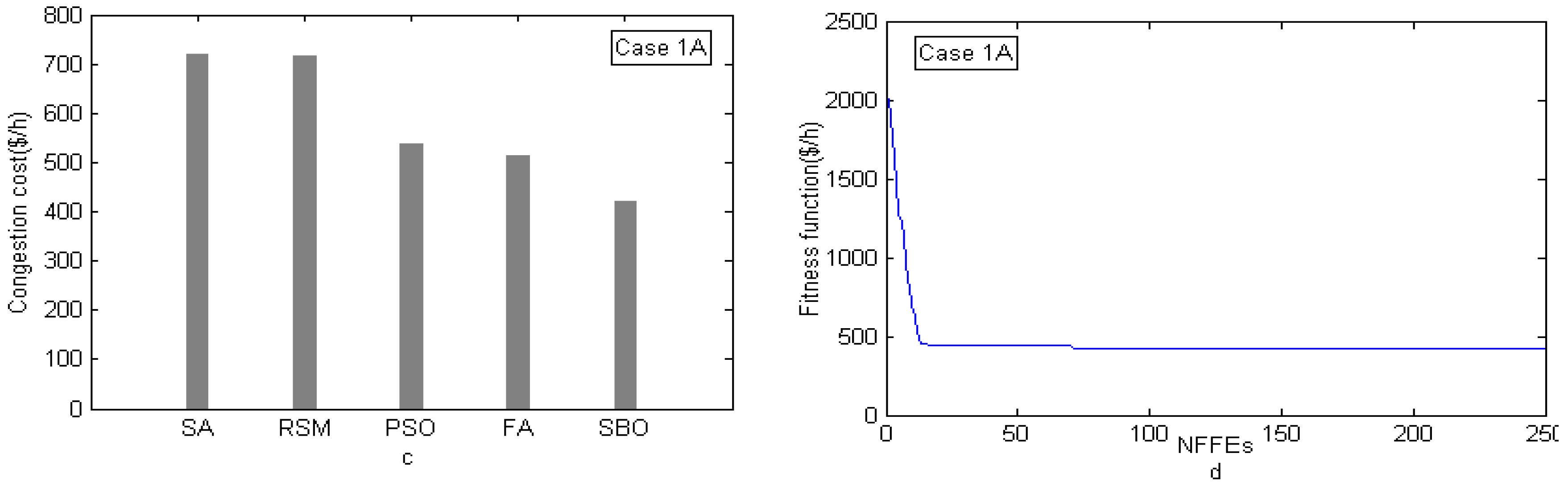
| 1A | 1–7 | 147.57 | 130 | 130 |
| 7–8 | 140.23 | 123.54 | 130 | |
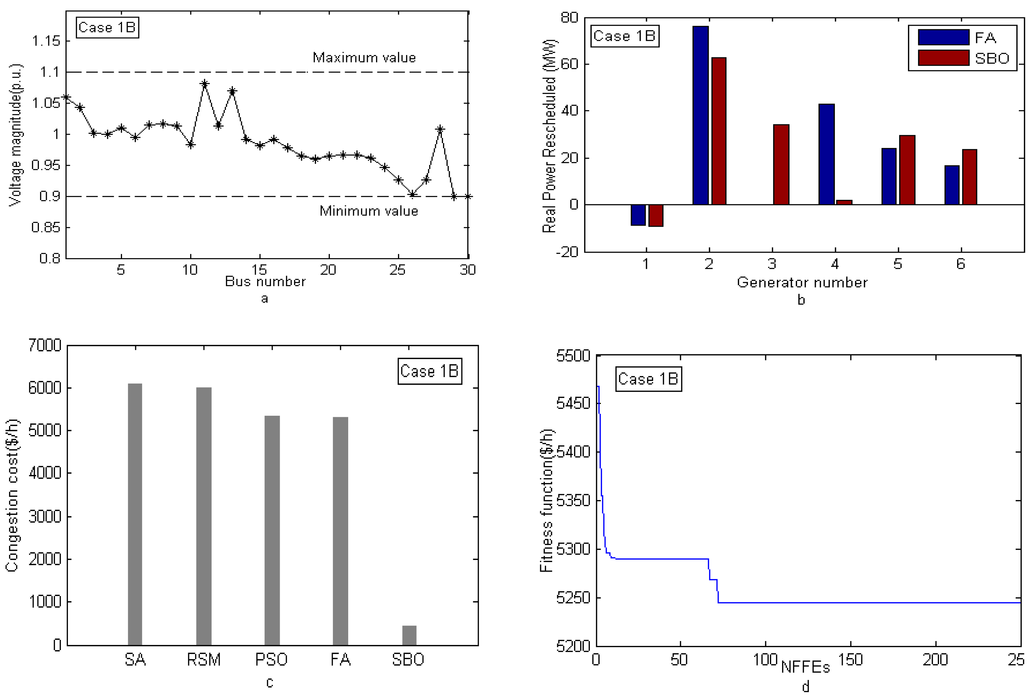
| 1B | 1–2 | 314.01 | 130 | 130 |
| 2–8 | 97.86 | 61.46 | 65 | |
| 2–9 | 103.66 | 64.39 | 65 | |
| 2A | 5–6 | 188.69 | 168.47 | 175 |
| 6–12 | 49.53 | 16.85 | 35 | |
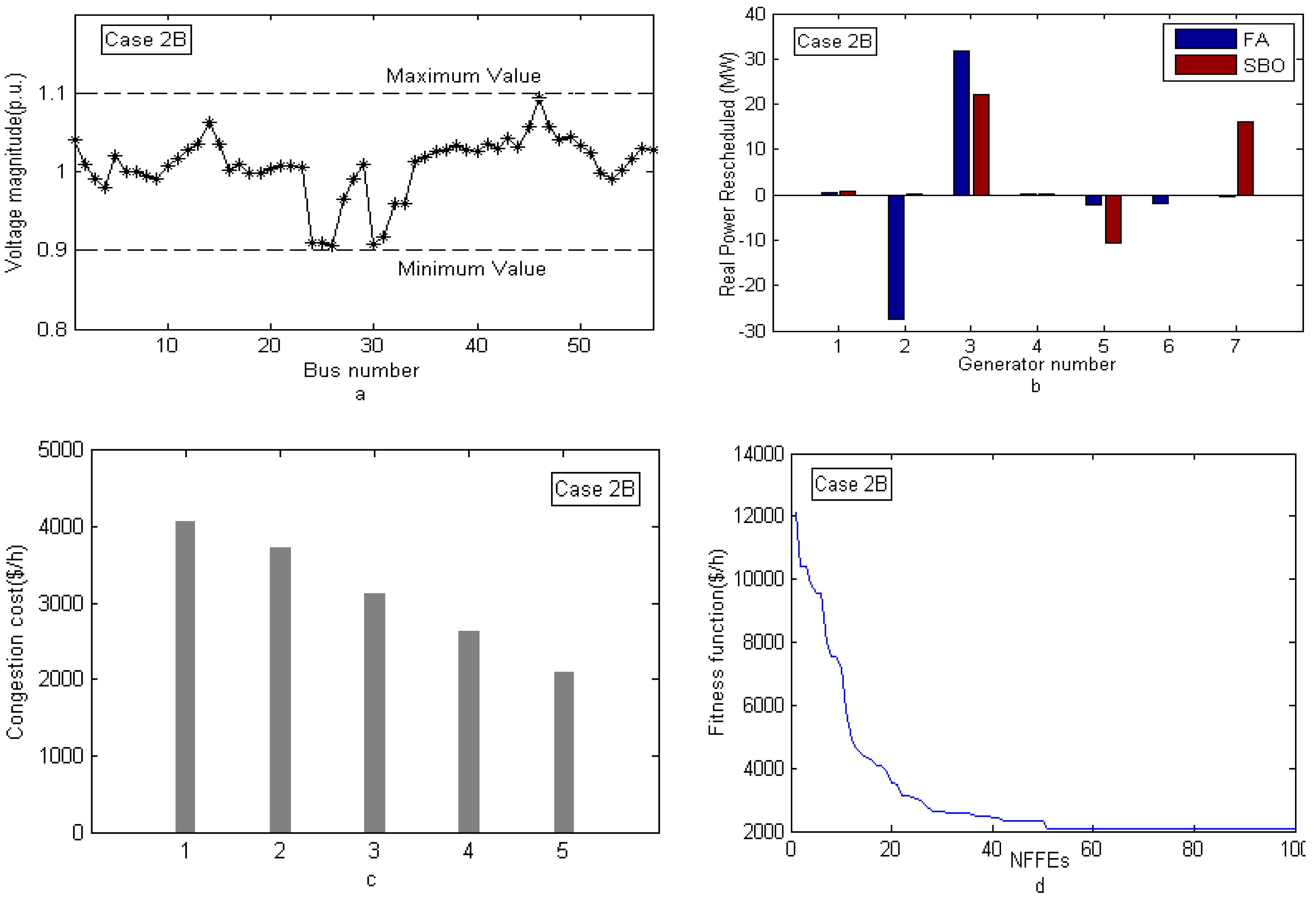
| 2B | 2–3 | 36.60 | 16.78 | 20 |
| 3 | 16–17 | 209.24 | 97.65 | 175 |
| 30–17 | 580.29 | 496.80 | 500 | |
| 8–30 | 363.52 | 143.08 | 175 | |
| Variables | SA [9] | RSM [9] | PSO [9] | FA [23] | SBO [Proposed] |
|---|---|---|---|---|---|
| Case 1A | |||||
| TC, $/h | 719.86 | 716.25 | 538.95 | 511.8737 | 421.58 |
| ΔPG1, MW | −9.076 | −8.808 | −8.61 | −8.7783 | −8.59617 |
| ΔPG2, MW | 3.133 | 2.647 | 10.4 | 15.0008 | 7.57019 |
| ΔPG3, MW | 3.234 | 2.953 | 3.03 | 0.1068 | 0.35246 |
| ΔPG4, MW | 2.968 | 3.063 | 0.02 | 0.0653 | 1.09699 |
| ΔPG5, MW | 2.954 | 2.913 | 0.85 | 0.1734 | 0.56891 |
| ΔPG6, MW | 2.443 | 2.952 | −0.01 | −0.6180 | 0.52286 |
| TRRG, MW | 23.809 | 23.33 | 22.93 | 24.7425 | 18.70758 |
| Case 1B | |||||
| TC, $/h | 6068.7 | 5988 | 5335.5 | 5304.40 | 5238.93 |
| ΔPG1, MW | NL | NL | NL | −8.5798 | −9.00148 |
| ΔPG2, MW | NL | NL | NL | 75.9954 | 62.90304 |
| ΔPG3, MW | NL | NL | NL | 0.0575 | 34.24745 |
| ΔPG4, MW | NL | NL | NL | 42.9944 | 2.05959 |
| ΔPG5, MW | NL | NL | NL | 23.8325 | 29.45485 |
| ΔPG6, MW | NL | NL | NL | 16.5144 | 23.47373 |
| TRRG, MW | 164.53 | 164.5 | 168 | 167.974 | 161.14013 |
| Variables | SA [9] | RSM [9] | PSO [9] | FA [23] | SBO [Proposed] |
|---|---|---|---|---|---|
| Case 2A | |||||
| TC, $/h | 7114.3 | 7967.1 | 6951.9 | 6050.1 | 5773.27 |
| ΔPG1, MW | 74.499 | 59.268 | 23.13 | 5.6351 | −0.05437 |
| ΔPG2, MW | 0 | 0 | 12.44 | 2.5230 | −11.72790 |
| ΔPG3, MW | −1.515 | 37.452 | 7.49 | 0.5098 | −5.81154 |
| ΔPG4, MW | 9.952 | −47.39 | −5.38 | 0.107 | −45.26118 |
| ΔPG5, MW | −85.92 | −52.12 | −81.21 | −39.1514 | −51.32093 |
| ΔPG6, MW | 0 | 0 | 0 | −35.1122 | −34.86761 |
| ΔPG7, MW | 0 | 0 | 39.03 | 62.1938 | −0.53486 |
| TRRG, MW | 171.87 | 196.23 | 168.78 | 145.227 | 144.57839 |
| Case 2B | |||||
| TC, $/h | 4072.9 | 3717.9 | 3117.6 | 2618.1 | 2084.78 |
| ΔPG1, MW | NL | NL | NL | 0.3704 | 0.76179 |
| ΔPG2, MW | NL | NL | NL | −27.5084 | 0.08662 |
| ΔPG3, MW | NL | NL | NL | 31.6294 | 22.04924 |
| ΔPG4, MW | NL | NL | NL | 0.3308 | 0.17019 |
| ΔPG5, MW | NL | NL | NL | −2.2549 | −10.50832 |
| ΔPG6, MW | NL | NL | NL | −1.9354 | −0.00000 |
| ΔPG7, MW | NL | NL | NL | −0.5101 | 16.00743 |
| TRRG, MW | 97.88 | 89.32 | 76.314 | 64.5393 | 49.58359 |
| Variables | EP [22] | RCGA [22] | PSO [22] | HPSO [22] | DE [22] | SBO [Proposed] |
|---|---|---|---|---|---|---|
| TC, $/h | 42,886 | 17,693 | 17,742 | 17,365 | 16,080 | 12,336.05 |
| ΔPG1 | 38.11 | 26.274 | 24.502 | 11.59 | 6.4705 | 6.35066 |
| ΔPG2 | 0 | 0 | 0 | 0 | 0 | 3.45815 |
| ΔPG3 | 63.06 | 31.422 | 1.0259 | 6.568 | 12.295 | 5.01763 |
| ΔPG4 | −7.48 | 11.349 | 1.3148 | −0.046 | −0.056 | 8.99506 |
| ΔPG5 | −200.6 | −219.3 | −21.82 | −207.7 | −208.1 | −203.28939 |
| ΔPG6 | 48.58 | 101.42 | 105.32 | 80.126 | 105.32 | 8.81232 |
| ΔPG7 | 0 | 0 | 0 | 0 | 0 | 22.22845 |
| ΔPG8 | 49.17 | 0.0029 | 16.815 | 6.0059 | 1.9946 | 0.61579 |
| ΔPG9 | 64.056 | 8.0582 | 23.665 | −0.239 | 1.2884 | 6.78422 |
| ΔPG10 | 0 | 0 | 0 | 0 | 0 | 2.32609 |
| ΔPG11 | 121.51 | 114.69 | 121.51 | 121.51 | 49.697 | −0.2996 |
| ΔPG12 | 25.918 | 116.31 | 116.31 | 108.06 | 113.29 | 1.06873 |
| ΔPG13 | 85.37 | 7.4155 | 3.0092 | 10.752 | 0.8125 | 0.62895 |
| ΔPG14 | 32.857 | −0.0019 | 0.0177 | −0.536 | 2.1836 | 4.24786 |
| ΔPG15 | 31.616 | 28.095 | 8.8665 | 11.254 | 89.669 | 12.42693 |
| ΔPG16 | 39.071 | 1.7508 | 7.1475 | 0.0731 | 0.7819 | 0.21691 |
| ΔPG17 | 37.552 | 0.0004 | 0.4916 | −0.394 | −0.041 | 0.49255 |
| ΔPG18 | 0 | 0 | 0 | 0 | 0 | 1.48727 |
| ΔPG19 | 0 | 0 | 0 | 0 | 0 | 0.46018 |
| ΔPG20 | 89.001 | 1.7478 | 6.0792 | 4.3096 | −0.089 | −0.34758 |
| ΔPG21 | 96.075 | 18.528 | 19.359 | 77.661 | 102.85 | −1.09116 |
| ΔPG22 | 93.828 | 33.426 | 36.798 | 72.901 | 7.3786 | −0.24492 |
| ΔPG23 | 0 | 0 | 0 | 0 | 0 | 0.36291 |
| ΔPG24 | 0 | 0 | 0 | 0 | 0 | 0.25945 |
| ΔPG25 | 0 | 0 | 0 | 0 | 0 | 1.53135 |
| ΔPG26 | 0 | 0 | 0 | 0 | 0 | −5.89327 |
| ΔPG27 | 0 | 0 | 0 | 0 | 0 | 0.3658 |
| ΔPG28 | 0 | 0 | 0 | 0 | 0 | −112.36346 |
| ΔPG29 | 0 | 0 | 0 | 0 | 0 | −6.58455 |
| ΔPG30 | −450.9 | 0 | 10.702 | 0.6525 | 4.904 | −4.10322 |
| ΔPG31 | 0 | 0 | 0 | 0 | 0 | 0.90951 |
| ΔPG32 | 0 | 0 | 0 | 0 | 0 | 0.40333 |
| ΔPG33 | 0 | 0 | 0 | 0 | 0 | 0.17212 |
| ΔPG34 | 0 | 0 | 0 | 0 | 0 | 0.78747 |
| ΔPG35 | 0 | 0 | 0 | 0 | 0 | 0.14819 |
| ΔPG36 | 0 | 0 | 0 | 0 | 0 | 0.18178 |
| ΔPG37 | 0 | 0 | 0 | 0 | 0 | −3.22489 |
| ΔPG38 | 0 | 0 | 0 | 0 | 0 | 0.32378 |
| ΔPG39 | 0 | 0 | 0 | 0 | 0 | −0.80088 |
| ΔPG40 | 0 | 0 | 0 | 0 | 0 | −74.35625 |
| ΔPG41 | 0 | 0 | 0 | 0 | 0 | 0.19709 |
| ΔPG42 | 0 | 0 | 0 | 0 | 0 | 0.15209 |
| ΔPG43 | 0 | 0 | 0 | 0 | 0 | 1.21754 |
| ΔPG44 | 0 | 0 | 0 | 0 | 0 | 0.13011 |
| ΔPG45 | 0 | 0 | 0 | 0 | 0 | −0.54271 |
| ΔPG46 | 0 | 0 | 0 | 0 | 0 | −3.72569 |
| ΔPG47 | 0 | 0 | 0 | 0 | 0 | 1.82584 |
| ΔPG48 | 0 | 0 | 0 | 0 | 0 | 0.36729 |
| ΔPG49 | 0 | 0 | 0 | 0 | 0 | 0.15896 |
| ΔPG50 | 0 | 0 | 0 | 0 | 0 | 0.99087 |
| ΔPG51 | 0 | 0 | 0 | 0 | 0 | −0.90559 |
| ΔPG52 | 0 | 0 | 0 | 0 | 0 | 0.27131 |
| ΔPG53 | 0 | 0 | 0 | 0 | 0 | 0.78541 |
| ΔPG54 | 0 | 0 | 0 | 0 | 0 | 1.05513 |
| TRRG | 1574.9 | 719.8998 | 717.7839 | 720.4816 | 707.3281 | 515.98823 |
| PSO | FFA | SBO |
|---|---|---|
| No. of particles = 40; Inertia weight = 0.9; = 0.4; = = 2 | Fireflies = 40; α and γ = 0 to 1; = 10 | Population size = 40, step size (α) = 0.94; z = 0.002; p = 0.05 |
| Maximum iterations = 150 | Maximum iterations = 150 | Maximum iterations = 150 |
© 2018 by the authors. Licensee MDPI, Basel, Switzerland. This article is an open access article distributed under the terms and conditions of the Creative Commons Attribution (CC BY) license (http://creativecommons.org/licenses/by/4.0/).
Share and Cite
Chintam, J.R.; Daniel, M. Real-Power Rescheduling of Generators for Congestion Management Using a Novel Satin Bowerbird Optimization Algorithm. Energies 2018, 11, 183. https://doi.org/10.3390/en11010183
Chintam JR, Daniel M. Real-Power Rescheduling of Generators for Congestion Management Using a Novel Satin Bowerbird Optimization Algorithm. Energies. 2018; 11(1):183. https://doi.org/10.3390/en11010183
Chicago/Turabian StyleChintam, Jagadeeswar Reddy, and Mary Daniel. 2018. "Real-Power Rescheduling of Generators for Congestion Management Using a Novel Satin Bowerbird Optimization Algorithm" Energies 11, no. 1: 183. https://doi.org/10.3390/en11010183
APA StyleChintam, J. R., & Daniel, M. (2018). Real-Power Rescheduling of Generators for Congestion Management Using a Novel Satin Bowerbird Optimization Algorithm. Energies, 11(1), 183. https://doi.org/10.3390/en11010183