Deep Belief Network Based Hybrid Model for Building Energy Consumption Prediction

Abstract

To enhance the prediction performance for building energy consumption, this paper presents a modified deep belief network (DBN) based hybrid model. The proposed hybrid model combines the outputs from the DBN model with the energy-consuming pattern to yield the final prediction results. The energy-consuming pattern in this study represents the periodicity property of building energy consumption and can be extracted from the observed historical energy consumption data. The residual data generated by removing the energy-consuming pattern from the original data are utilized to train the modified DBN model. The training of the modified DBN includes two steps, the first one of which adopts the contrastive divergence (CD) algorithm to optimize the hidden parameters in a pre-train way, while the second one determines the output weighting vector by the least squares method. The proposed hybrid model is applied to two kinds of building energy consumption data sets that have different energy-consuming patterns (daily-periodicity and weekly-periodicity). In order to examine the advantages of the proposed model, four popular artificial intelligence methods—the backward propagation neural network (BPNN), the generalized radial basis function neural network (GRBFNN), the extreme learning machine (ELM), and the support vector regressor (SVR) are chosen as the comparative approaches. Experimental results demonstrate that the proposed DBN based hybrid model has the best performance compared with the comparative techniques. Another thing to be mentioned is that all the predictors constructed by utilizing the energy-consuming patterns perform better than those designed only by the original data. This verifies the usefulness of the incorporation of the energy-consuming patterns. The proposed approach can also be extended and applied to some other similar prediction problems that have periodicity patterns, e.g., the traffic flow forecasting and the electricity consumption prediction.

1. Introduction

With the growth of population and the development of economy, more and more energy is consumed in the residential and office buildings. Building energy conservation plays an important role in the sustainable development of economy. However, some ubiquitous issues, e.g., the poor building management and the unreasonable task scheduling, are impeding the efficiency of the energy conservation policies. To improve the building management and the task scheduling of building equipment, one way is to provide accurate prediction of the building energy consumption.

Nowadays, numerous data-driven artificial intelligence approaches have been proposed for building energy consumption prediction. In [1], the random forest and the artificial neural network (ANN) were applied to the high-resolution prediction of building energy consumption, and their experimental results demonstrated that both models have comparable predictive power. In [2], a hybrid model combining different machine learning algorithms was presented for optimizing energy consumption of residential buildings under the consideration of both continuous and discrete parameters of energy. In [3], the extreme learning machine (ELM) was used to estimate the building energy consumption, and simulation results indicated that the ELM performed better than the genetic programming (GP) and the ANN. In [4], the clusterwise regression method, also known as the latent class regression, which integrates clustering and regression, was utilized to the accurate and stable prediction of building energy consumption data. In [5], the feasibility and applicability of support vector machine (SVM) for building energy consumption prediction were examined in a tropical region. Moreover, in [6,7,8,9], a variation of SVM, the support vector regressor (SVR) was proposed for forecasting the building energy consumption and the electric load. Furthermore, in [10], a novel machine learning model was constructed for estimating the commercial building energy consumption.

The historical building energy consumption data have high levels of uncertainties and randomness due to the influence of the human distribution, the thermal environment, the weather conditions and the working hours in buildings. Thus, there still exists the need to improve the prediction precision for this application. To realize this objective, we can take two strategies into account. The first strategy is to adopt the more powerful modeling methods to learn the information hidden in the historical data, while the other one is to incorporate the knowledge or patterns from our experience or data into the prediction models.

On the one hand, the deep learning technique provides us one very powerful tool for constructing the prediction model. In the deep learning models, more representative features can be extracted from the lowest layer to the highest layer [11,12]. Until today, this miraculous technique has been widely used in various fields. In [13], a novel predictor, the stacked autoencoder Levenberg–Marquardt model was constructed for the prediction of traffic flow. In [14], an extreme deep learning approach that integrates the stacked autoencoder (SAE) with the ELM was proposed for building energy consumption prediction. In [15], the deep learning was employed as an ensemble technique for cancer detection. In [16], the deep convolutional neural network (CNN) was utilized for face photo-sketch recognition. In [17], a deep learning approach, the Gaussian–Bernoulli restricted Boltzmann machine (RBM) was applied to 3D shape classification through using spectral graph wavelets and the bag-of-features paradigm. In [18], the deep belief network (DBN) was applied to solve the natural language understanding problem. Furthermore, in [19], the DBN was utilized to fuse the virtues of multiple acoustic features for improving the robustness of voice activity detection. As one popular deep learning method, the DBN has shown its superiority in machine learning and artificial intelligence. This study will adopt and modify the DBN to make it be suitable for the prediction of building energy consumption.

On the other hand, knowledge or patterns from our experience can provide additional information for the design of the prediction models. In [20,21,22], different kinds of prior knowledge were incorporated into the SVM models. In [23], the knowledge of symmetry was encoded into the type-2 fuzzy logic model to enhance its performance. In [24,25], the knowledge of monotonicity was incorporated into the fuzzy inference systems to assure the models’ monotonic input–output mappings. In [26,27,28,29], how to encode the knowledge into neural networks was discussed. As shown in these studies, through incorporating the knowledge or pattern, the constructed machine learning models will yield better performance and have significantly improved generalization ability.

From the above discussion, both the deep learning method and the domain knowledge are helpful for the prediction models’ performance improvement. Following this idea, this study tries to present a hybrid model that combines the DBN model with the periodicity knowledge of the building energy consumption to further improve the prediction accuracy. The final prediction results of the proposed hybrid model are obtained by combining the outputs from the modified DBN model and the energy-consuming pattern model. Here, the energy-consuming pattern represents the periodicity property of building energy consumption and can be extracted from the observed historical energy consumption data. In this study, firstly, the structure of the proposed hybrid model will be presented, and how to extract the energy-consuming pattern will be demonstrated. Then, the training algorithm for the modified DBN model will be provided. The learning of the DBN model mainly includes two steps, which firstly optimizes the hidden parameters by the contrastive divergence (CD) algorithm in a pre-train way, and then determines the output weighting vector by the least squares method. Furthermore, the proposed hybrid model will be applied to the prediction of the energy consumption in two kinds of buildings that have different energy-consuming patterns (daily-periodicity and weekly-periodicity). Additionally, to show the superiority of the proposed hybrid model, comparisons with four popular artificial intelligence methods—the backward propagation neural network (BPNN), the generalized radial basis function neural network (GRBFNN), the extreme learning machine (ELM), and the support vector regressor (SVR) will be made. From the comparison results, we can observe that all the predictors (DBN, BPNN, GRBFNN, ELM and SVR) designed using both the periodicity knowledge and residual data perform much better than those designed only by the original data. Hence, we can judge that the periodicity knowledge is quite useful for improving the prediction performance in this application. The experiments also show that, among all the prediction models, the proposed DBN based hybrid model has the best performance.

The rest of this paper is as follows. In Section 2, the deep belief network will be reviewed. In Section 3, the proposed hybrid model will be presented firstly, and then the modified DBN will be provided. In Section 4, two energy consumption prediction experiments for buildings that have different energy-consuming patterns will be done. In addition, the experimental and comparison results will be given. Finally, in Section 5, the conclusions of this paper will be drawn.

2. Introduction of DBN

The DBN is a stack of restricted Boltzmann machine (RBM) [11,30]. Therefore, for better understanding, we will introduce the RBM before the introduction of the DBN in this section.

2.1. Restricted Boltzmann Machine

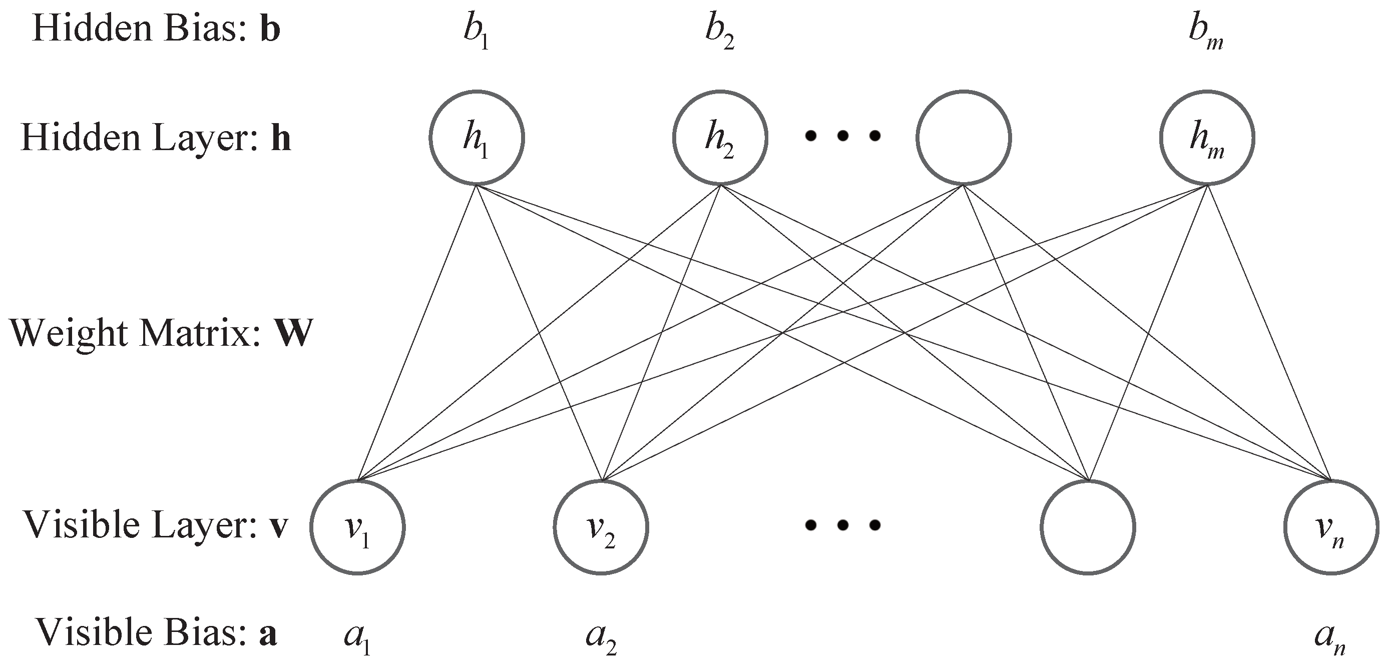
The structure of a typical RBM model is shown in Figure 1. The RBM is an undirected, bipartite graphical model, which consists of the visible (input) layer and the hidden (output) layer. The visible layer and the hidden layer are respectively made up of n visible units and m hidden units, and there is a bias in each unit. Moreover, there are no interconnection within the visible layer or the hidden layer [31].

The activation probability of the jth hidden unit can be computed as follows when a visible vector $\mathit{v}(v_1,\dots ,v_i,\dots ,v_n)$ is given [32]

$$\begin{array}{c}\hfill p(h_j=1|\mathit{v})=\sigma (b_j+\sum _{i=1}^n{v}_i{w}_{ij}),\end{array}$$

(1)

where $\sigma (·)$ is the sigmoid function, $w_{ij}$ is the connection weight between the ith visible unit and jth hidden unit, and $b_j$ is the bias of the jth hidden unit.

Similarly, when a hidden vector $\mathit{h}(h_1,\dots ,h_j,\dots ,h_m)$ is known, the activation probability of the ith visible unit can be computed as follows:

$$\begin{array}{c}\hfill p(v_i=1|\mathit{h})=\sigma (a_i+\sum _{j=1}^m{h}_j{w}_{ij}),\end{array}$$

(2)

where $i=1,2,\dots ,n$, and $a_i$ is the bias of the ith visible unit.

Hinton et al. [33] have proposed the contrastive divergence (CD) algorithm to optimize the RBM. The CD algorithm based RBM’s iterative learning procedures for binomial units are listed as follows [32].

Step 1:

Initialize the number of visible units n, the number of hidden units m, the number of training data N, the weighting matrix $\mathit{W}$, the visible bias vector $\mathit{a}$, the hidden bias vector $\mathit{b}$ and the learning rate $ϵ$.

Step 2:

Assign a sample $\mathit{x}$ from the training data to be the initial state ${\mathit{v}}_{\mathbf{0}}$ of the visible layer.

Step 3:

Calculate $p(h_{0j}=1|{\mathit{v}}_{\mathbf{0}})$ according to Equation (1), and extract $h_{0j}\in \{0,1\}$ from the conditional distribution $p(h_{0j}=1|{\mathit{v}}_{\mathbf{0}})$, where $j=1,2,\dots ,m$.

Step 4:

Calculate $p(v_{1i}=1|{\mathit{h}}_{\mathbf{0}})$ according to Equation (2), and extract $v_{1i}\in \{0,1\}$ from the conditional distribution $p(v_{1i}=1|{\mathit{h}}_{\mathbf{0}})$, where $i=1,2,\dots ,n$.

Step 5:

Calculate $p(h_{1j}=1|{\mathit{v}}_{\mathbf{1}})$ according to Equation (1).

Step 6:

Update the parameters according to the following equations:

$\mathit{W}=\mathit{W}+ϵ(p({\mathit{h}}_0=1|{\mathit{v}}_0){{\mathit{v}}_{\mathbf{0}}}^{\mathtt{T}}-p({\mathit{h}}_1=1|{\mathit{v}}_1){{\mathit{v}}_{\mathbf{1}}}^{\mathtt{T}}),$

$\mathit{a}=\mathit{a}+ϵ({\mathit{v}}_0-{\mathit{v}}_1),$

$\mathit{b}=\mathit{b}+ϵ(p({\mathit{h}}_0=1|{\mathit{v}}_0)-p({\mathit{h}}_1=1|{\mathit{v}}_1)).$

Step 7:

Assign another sample from the training data to be the initial state ${\mathit{v}}_{\mathbf{0}}$ of the visible layer, and iterate Steps 3 to 7 until all the N training data have been used.

2.2. Deep Belief Network

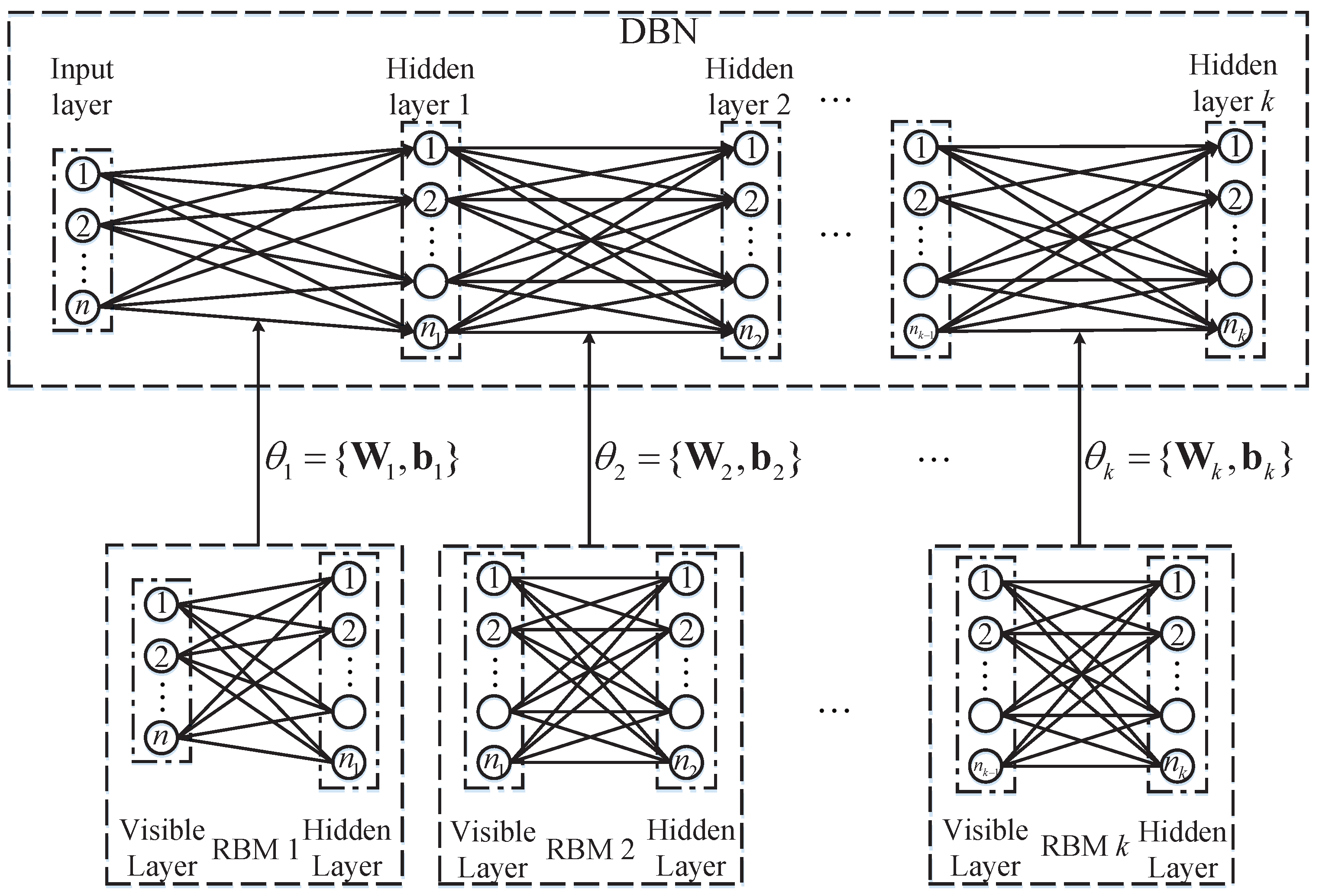
As aforementioned, the DBN as a miraculous deep model is a stack of RBMs [11,30,34,35]. Figure 2 illustrates the architecture of the DBN with k hidden layers and its layer-wise pre-training process.

The activation of the kth hidden layer with respect to input sample $\mathit{x}$ can be computed as

$$\begin{array}{c}\hfill {\mathit{A}}_k(\mathit{x})=\sigma \left({\mathit{b}}_k+{\mathit{W}}_k\sigma \left(\cdots +{\mathit{W}}_2\sigma \left({\mathit{b}}_1+{\mathit{W}}_1\mathit{x}\right)\right)\right),\end{array}$$

(3)

where ${\mathbf{W}}_u$ and ${\mathit{b}}_u$ ($u=1,2,\dots ,k$) are, respectively, the weighting matrices and hidden bias vectors of the uth RBM. Furthermore, $\sigma$ is the logistic sigmoid function $\sigma (x)=1/(1+e^{-x})$.

In order to obtain better feature representation, the DBN utilizes deep architecture and adopts the layer-wise pre-training to optimize the inter-layer weighting matrix [11]. The training algorithm of the DBN will be given in the next section in detail.

3. The Proposed Hybrid Model

In this section, the structure of the hybrid model will be proposed first. Then, the extraction of the energy-consuming pattern and the generation of the residual data will be given. Finally, the modified DBN (MDBN) and its training algorithm will be presented.

To begin, we assume that we have collected the sampling data for M consecutive days, and, in each day, we collected T data points. Then, sampled time series of energy consumption data can be written as a series of 1D vectors as

$$\begin{array}{c}\hfill \mathit{Y}=\left\{{\mathit{Y}}_1,{\mathit{Y}}_2,\dots ,{\mathit{Y}}_M\right\},\end{array}$$

(4)

where

$$\begin{array}{c}\hfill \begin{array}{cc}\hfill {\mathit{Y}}_1& =[y_1(1),y_1(2),\dots ,y_1(T)],\hfill \\ & ⋮\\ \hfill {\mathit{Y}}_M& =[y_M(1),y_M(2),\dots ,y_M(T)],\hfill \end{array}\end{array}$$

(5)

and T is the sampling number per day.

3.1. Structure of the Hybrid Model

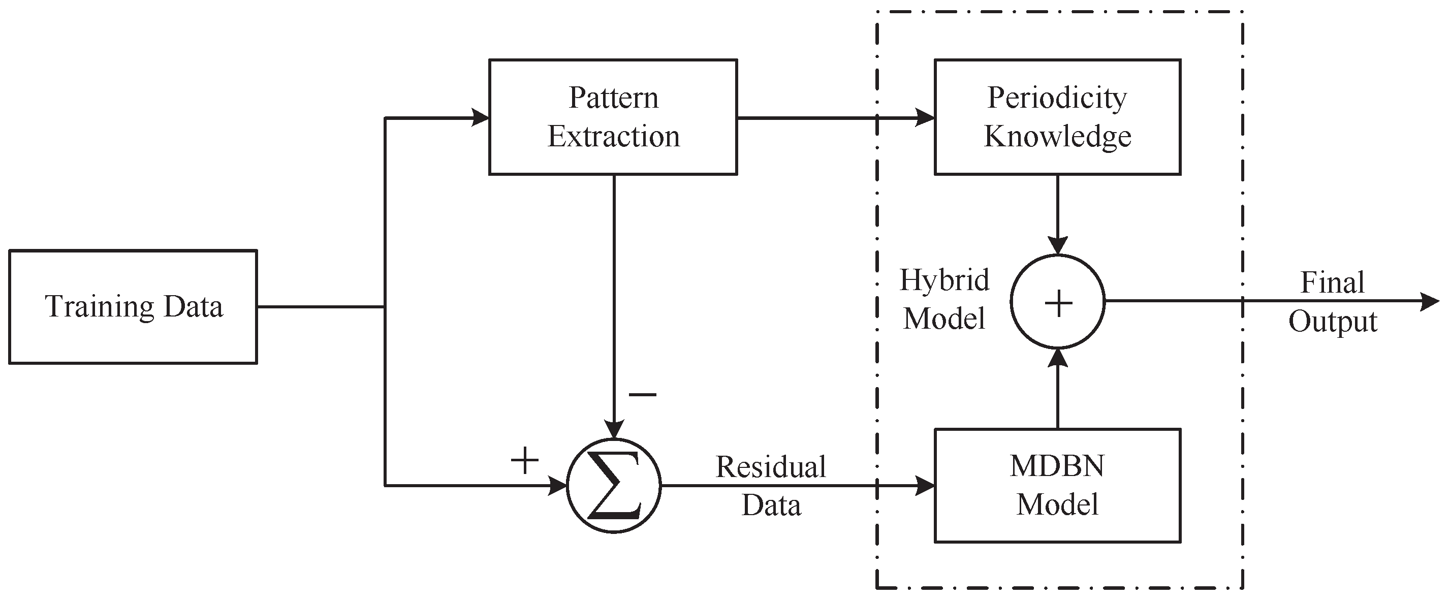
The hybrid model combines the modified DBN (MDBN) model with the periodicity knowledge of the building energy consumption to obtain better prediction accuracy. The design procedure of the proposed model is depicted in Figure 3 and is also given as follows:

Step 1:

Extract the energy-consuming pattern as the periodicity knowledge from the training data.

Step 2:

Remove the energy-consuming pattern from the training data to generate the residual data.

Step 3:

Utilize the residual data to train the MDBN model.

Step 4:

Combine the outputs from the MDBN model with the periodicity knowledge to obtain the final prediction results of the hybrid model.

It is obvious that the extraction of the energy-consuming pattern, the generation of the residual data and the construction of the MDBN model are crucial in order to build the proposed hybrid model. Consequently, we will introduce them in detail in the following subsections.

3.2. Extraction of the Energy-Consuming Patterns and Generation of the Residual Data

Obviously, various regular patterns of energy consumption (e.g., daily-periodicity, weekly-periodicity, monthly-periodicity and even yearly-periodicity) exist in different kinds of buildings. In this study, we will take the daily-periodic and the weekly-periodic energy-consuming patterns as examples to introduce the method for extracting them from the original data.

3.2.1. The Daily-Periodic Pattern

For daily-periodic energy-consuming pattern, it can be extracted from the original time series by the following equation:

$$\begin{array}{c}\hfill {\overline{\mathit{Y}}}_{Ave}=\left[\frac{1}{M}\sum _{z=1}^M{y}_z(1),\frac{1}{M}\sum _{z=1}^M{y}_z(2),\dots ,\frac{1}{M}\sum _{z=1}^M{y}_z(T)\right].\end{array}$$

(6)

Then, the residual time series ${\mathit{Y}}_{Res}$ of the data set after removing the daily-periodic pattern can be generated as

$$\begin{array}{c}\hfill {\mathit{Y}}_{Res}=\left\{{\mathit{Y}}_1-{\overline{\mathit{Y}}}_{Ave},{\mathit{Y}}_2-{\overline{\mathit{Y}}}_{Ave},\cdots ,{\mathit{Y}}_M-{\overline{\mathit{Y}}}_{Ave}\right\}.\end{array}$$

(7)

3.2.2. The Weekly-Periodic Pattern

Being different from the daily-periodic energy-consuming pattern, the weekly-periodic energy-consuming pattern includes two parts, which are the patterns of weekdays and weekends. The weekday pattern and the weekend pattern can be respectively computed as

$$\begin{array}{c}\hfill {\overline{\mathit{Y}}}_{Weekday}=\left[\frac{1}{M_1}\sum _{z=1}^{M_1}{p}_z(1),\frac{1}{M_1}\sum _{z=1}^{M_1}{p}_z(2),\dots ,\frac{1}{M_1}\sum _{z=1}^{M_1}{p}_z(T)\right],\end{array}$$

(8)

$$\begin{array}{c}\hfill {\overline{\mathit{Y}}}_{Weekend}=\left[\frac{1}{M_2}\sum _{z=1}^{M_2}{q}_z(1),\frac{1}{M_2}\sum _{z=1}^{M_2}{q}_z(2),\dots ,\frac{1}{M_2}\sum _{z=1}^{M_2}{q}_z(T)\right],\end{array}$$

(9)

where

$$\begin{array}{c}\hfill \mathit{P}=\left\{{\mathit{P}}_1=[p_1(1),\dots ,p_1(T)],\dots ,{\mathit{P}}_{M_1}=[p_{M_1}(1),\dots ,p_{M_1}(T)]\right\},\end{array}$$

(10)

$$\begin{array}{c}\hfill \mathit{Q}=\left\{{\mathit{Q}}_1=[q_1(1),\dots ,q_1(T)],\dots ,{\mathit{Q}}_{M_2}=[q_{M_2}(1),\dots ,q_{M_2}(T)]\right\},\end{array}$$

(11)

are, respectively, the data sets of weekdays and weekends, and $M_1+M_2=M$.

Then, to generate the residual time series ${\mathit{Y}}_{Res}$ for the building energy consumption data set, we use the following rules:

$$\begin{array}{cc}If{\mathit{Y}}_z\in \mathit{P},\hfill & \hfill then{\mathit{Y}}_{z,Res}={\mathit{Y}}_z-{\overline{\mathit{Y}}}_{Weekday},\end{array}$$

(12)

$$\begin{array}{cc}If{\mathit{Y}}_z\in \mathit{Q},\hfill & \hfill then{\mathit{Y}}_{z,Res}={\mathit{Y}}_z-{\overline{\mathit{Y}}}_{Weekend},\end{array}$$

(13)

where $z=1,2,\dots ,M$.

Subsequently, ${\mathit{Y}}_{Res}$ can be written as

$$\begin{array}{c}\hfill {\mathit{Y}}_{Res}=\left\{{\mathit{Y}}_{1,Res},{\mathit{Y}}_{2,Res},\dots ,{\mathit{Y}}_{M,Res}\right\}.\end{array}$$

(14)

3.3. Modified DBN and Its Training Algorithm

In this subsection, the structure of the MDBN will be shown firstly. Then, the pre-training process of the DBN part will be described in detail. At last, the least squares method will be employed to determine the weighting vector of the regression part.

3.3.1. Structure of the MDBN

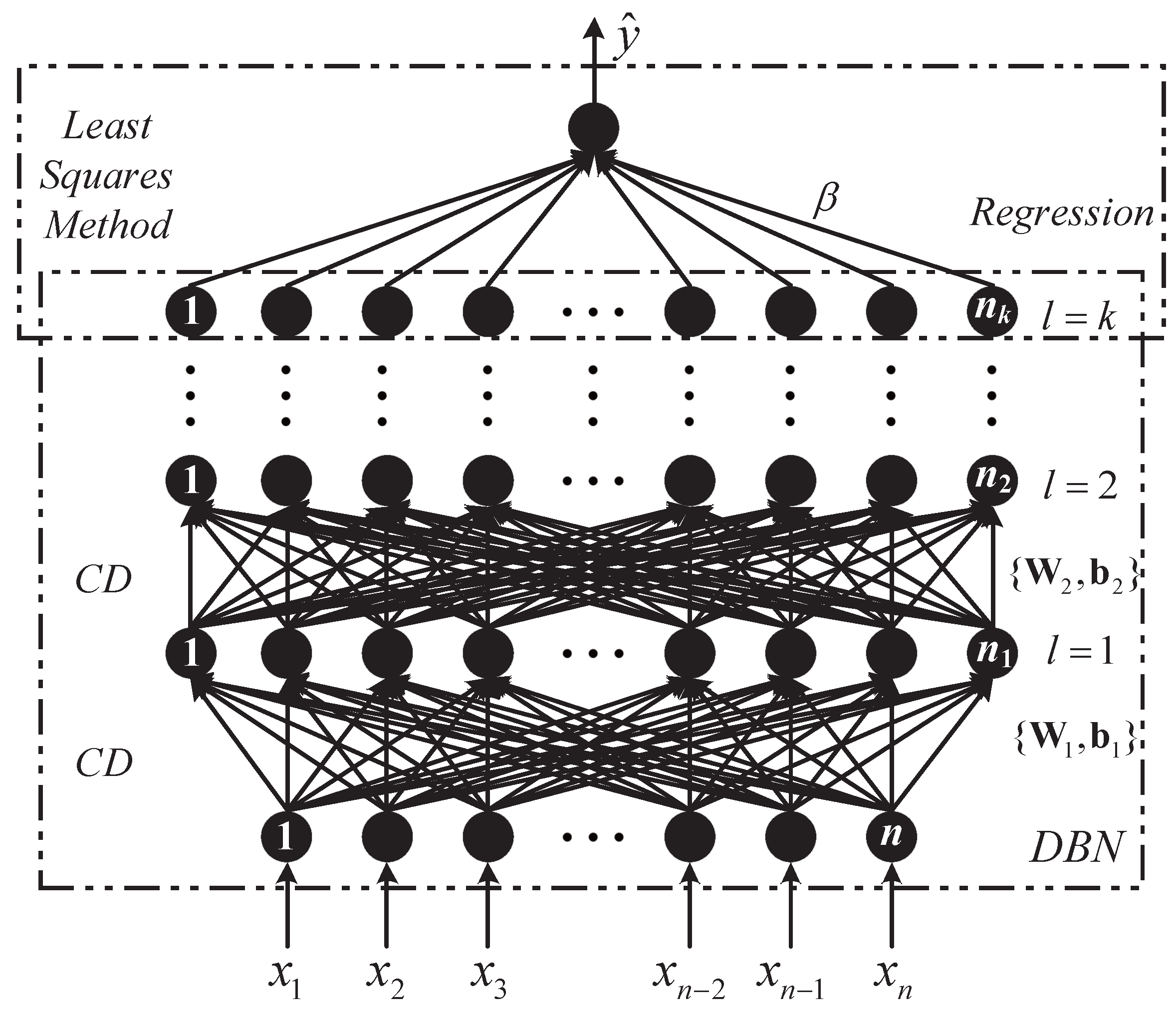
In the parameter optimization of the traditional DBNs, the CD algorithm is adopted to pre-train the parameters of multiple RBMs, and the BP algorithm is used to finely tune the parameters of the whole network. In this paper, we add an extra layer as the regression part to the DBN to realize the prediction function. Thus, we call it the modified DBN (MDBN). The structure of the MDBN is demonstrated in Figure 4. In addition, we propose a training algorithm that combines the CD algorithm with the least squares method for the learning of the MDBN model.

We divide the training process of the MDBN into two steps. The first step adopts the contrastive divergence algorithm to optimize the hidden parameters in a pre-train way, while the second one determines the output weighting vector by the least squares method. The detailed description will be given as below.

3.3.2. Pre-Training of the DBN Part

Generally speaking, with the number of hidden layers increasing, the effectiveness of the BP algorithm for optimizing the parameters of the deep neural network is getting lower and lower because of the gradient divergence. Fortunately, Hinton et al. [11] proposed a fast learning algorithm for the DBN. This novel approach realizes layer-wise pre-train of the multiple RBMs in the DBN in a bottom-up way as described below:

Step 1:

Initialize the number of hidden layers k, the number of the training data N and the initial sequence number of hidden layer $u=2$.

Step 2:

Assign a sample $\mathit{x}$ from the training data to be the input data of the DBN.

Step 3:

Regard the input layer and the first hidden layer of the DBN as an RBM, and compute the activation ${\mathit{A}}_1(\mathit{x})$ by Equation (3) when the training process of this RBM is finished.

Step 4:

Regard the uth and the $(u+1)$th hidden layer as an RBM with the input ${\mathit{A}}_{u-1}(\mathit{x})$, and compute the activation ${\mathit{A}}_u(\mathit{x})$ by Equation (3) when the training process of this RBM is completed.

Step 5:

Let $u=u+1$, and iterate Step 4 until $u>k$.

Step 6:

Use the ${\mathit{A}}_k(\mathit{x})$ as the input of the regression part.

Step 7:

Assign another sample from the training data as the input data of the DBN, and iterate Step 3 to 7 until all the N training data have been assigned.

3.3.3. Least Squares Learning of the Regression Part

Suppose that the training set is $\aleph =\{({\mathit{x}}^{(l)},y^{(l)})|{\mathit{x}}^{(l)}\in {\mathbf{R}}^n,y^{(l)}\in \mathbf{R},l=1,\cdots ,N\}$. As aforementioned, once the pre-training of the DBN part is completed, the activation of the final hidden layer of the MDBN with respect to the input ${\mathit{x}}^{(l)}$ can be obtained to be ${\mathit{A}}_k({\mathit{x}}^{(l)}),$ where $l=1,2,\dots ,N$. Furthermore, the activation of the final hidden layer of the MDBN with respect to all the N training data can be written in the matrix form as

$$\begin{array}{cc}\hfill {\mathit{A}}_k(\mathit{X})& ={[{\mathit{A}}_k({\mathit{x}}^{(1)}),{\mathit{A}}_k({\mathit{x}}^{(2)}),\cdots ,{\mathit{A}}_k({\mathit{x}}^{(N)})]}^{\mathtt{T}}\hfill \\ & ={\left[\begin{array}{c}\sigma \left({\mathit{b}}_k+{\mathit{w}}_k\sigma \left(\cdots +{\mathit{w}}_2\sigma \left({\mathit{b}}_1+{\mathit{w}}_1{\mathit{x}}^{(1)}\right)\right)\right)\\ \sigma \left({\mathit{b}}_k+{\mathit{w}}_k\sigma \left(\cdots +{\mathit{w}}_2\sigma \left({\mathit{b}}_1+{\mathit{w}}_1{\mathit{x}}^{(2)}\right)\right)\right)\\ ⋮\\ \sigma \left({\mathit{b}}_k+{\mathit{w}}_k\sigma \left(\cdots +{\mathit{w}}_2\sigma \left({\mathit{b}}_1+{\mathit{w}}_1{\mathit{x}}^{(N)}\right)\right)\right)\end{array}\right]}_{N\times n_k},\hfill \end{array}$$

(15)

where $n_k$ is the number of neurons of the kth hidden layer.

We always expect that each actual value $y^{(l)}$ with respect to ${\mathit{x}}^{(l)}$ can be approximated by the output ${\widehat{y}}^{(l)}$ of the predictor with no error. This expectation can be mathematically expressed as

$$\begin{array}{c}\hfill \sum _{l=1}^N\parallel {\widehat{y}}^{(l)}-y^{(l)}\parallel =0,\end{array}$$

(16)

where ${\widehat{y}}^{(l)}$ is the output of the MDBN and can be computed as

$$\begin{array}{c}\hfill {\widehat{y}}^{(l)}={\mathit{A}}_k({\mathit{x}}^{(l)})\mathit{\beta }\end{array}$$

(17)

in which $\mathit{\beta }$ is the output weighting vector and can be expressed as

$$\begin{array}{c}\hfill \mathit{\beta }={[{\mathit{\beta }}_1,{\mathit{\beta }}_2,\cdots ,{\mathit{\beta }}_{n_k}]}_{n_k\times 1}^{\mathtt{T}}.\end{array}$$

(18)

Then, Equation (16) can be rewritten in the matrix form as

$$\begin{array}{c}\hfill {\mathit{A}}_k(\mathit{X})\mathit{\beta }=\mathit{Y},\end{array}$$

(19)

where

$$\begin{array}{cc}\hfill \mathit{Y}& ={[y^{(1)},y^{(2)},\dots ,y^{(N)}]}_{N\times 1}^{\mathtt{T}}.\hfill \end{array}$$

(20)

From Equation (19), the output weighting vector $\mathit{\beta }$ can be derived by the least squares method as [36,37,38,39]

$$\begin{array}{c}\hfill \mathit{\beta }={\mathit{A}}_k{(\mathit{X})}^{†}\mathit{Y},\end{array}$$

(21)

where ${\mathit{A}}_k{(\mathit{X})}^{†}$ is the Moore–Penrose generalized inverse of ${\mathit{A}}_k(\mathit{X})$.

4. Experiments

In this section, first of all, four comparative artificial intelligence approaches will be introduced briefly. Next, the applied data sets and experimental setting will be discussed. Then, the proposed hybrid model will be applied to the prediction of the energy consumption in a retail store and an office building that respectively have daily-periodic and weekly-periodic energy-consuming patterns. Finally, we will give the comparisons and discussions of the experiments.

4.1. Introduction of the Comparative Approaches

To make a quantitative assessment of the proposed MDBN based hybrid model, four popular artificial intelligence approaches, the BPNN, GRBFNN, ELM, and SVR, are chosen as the comparative approaches and introduced briefly below.

4.1.1. Backward Propagation Neural Network

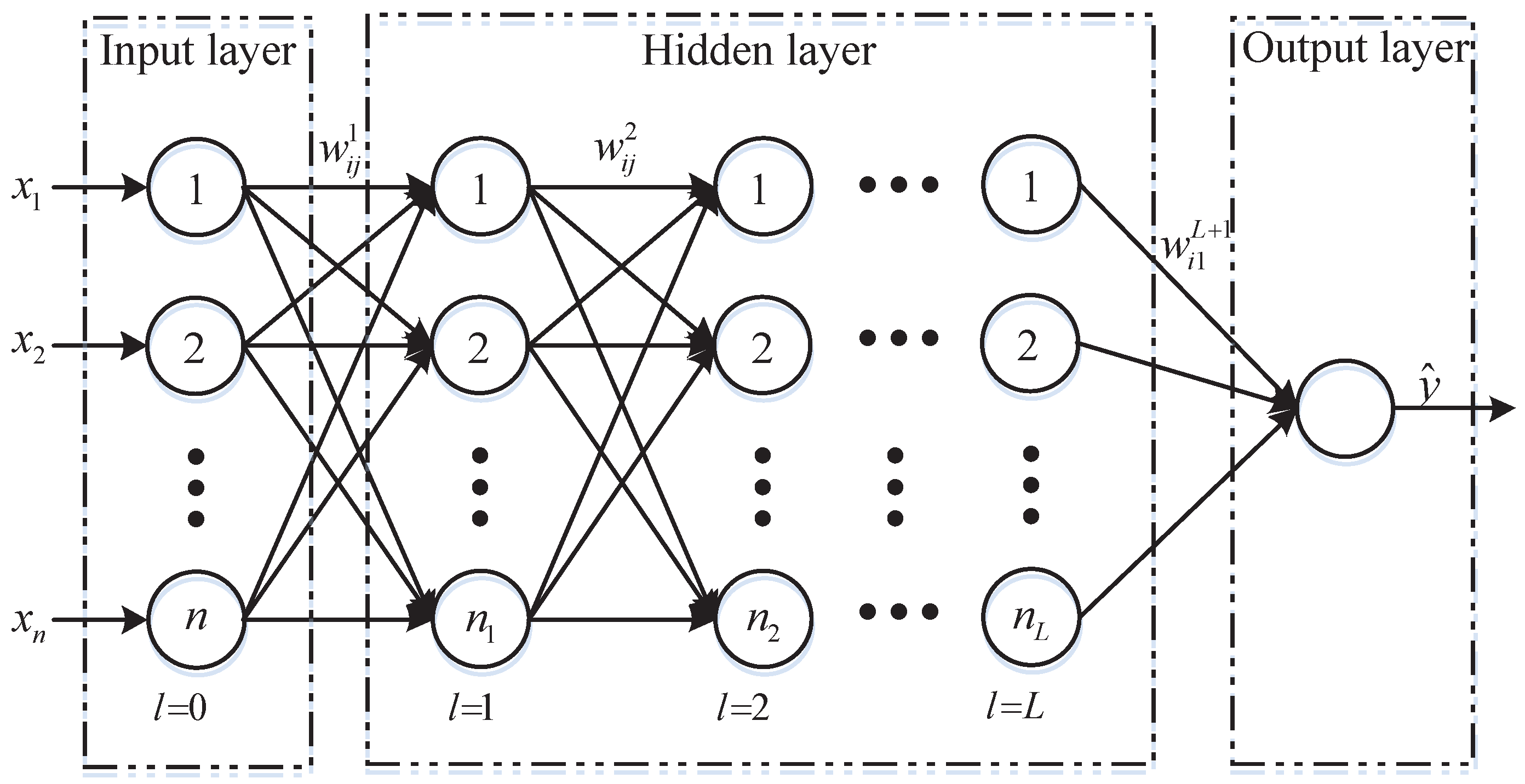
The structure of BPNN with L hidden layers is demonstrated in Figure 5. The BPNN as one popular kind of ANN adopts back propagation algorithm to obtain the optimal weighting parameters of the whole network [40,41,42].

As shown in Figure 5, the final output of the network can be expressed as [40,41,42]

$$\begin{array}{c}\hfill \widehat{y}=f(\sum _{s=1}^{n_L}{w}_{s1}^{L+1}\cdots f(\sum _{j=1}^{n_1}{w}_{jk}^{2}f(\sum _{i=1}^n{w}_{ij}^1{x}_i))),\end{array}$$

(22)

where $w_{ij}^k$ is the connection weight between the ith unit of kth layer and the jth unit of $(k+1)$th layer, and $f(·)$ is the logistic sigmoid function.

In order to obtain the optimal parameters of the BPNN, the Backward Propagation (BP) algorithm is adopted to minimize the following cost function for each training data point

$$\begin{array}{c}\hfill E(t,\mathit{w})={({\widehat{y}}^{(t)}-y^{(t)})}^2,\end{array}$$

(23)

where ${\widehat{y}}^{(t)}$ and $y^{(t)}$ are the predicted and actual values with respect to the input ${\mathit{x}}^{(t)}$.

The update rule for the weight $w_{ij}^k$ can be expressed as

$$\begin{array}{c}\hfill w_{ij}^k(t+1)=w_{ij}^k(t)-\eta \frac{\partial E(t,\mathit{w})}{\partial w_{ij}^k},\end{array}$$

(24)

where $\eta$ is the learning rate, and $\frac{\partial E(t,\mathit{w})}{\partial w_{ij}^k}$ is the gradient of the parameter $w_{ij}^k$, and can be calculated by the backward propagation of the errors.

The BP algorithm has two phases—forward propagation and weight update. In the forward propagation stage, when an input vector is input to the NN, it is propagated forward through the whole network until it reaches the output layer. Then, the error between the output of the network and the desired output is computed. In the weight update phase, the error is propagated from the output layer back through the whole network, until each neuron has an associated error value that can reflect its contribution to the original output. These error values are then used to calculate the gradients of the loss function that are fed to the update rules to renew the weights [40,41,42].

4.1.2. Generalized Radial Basis Function Neural Network

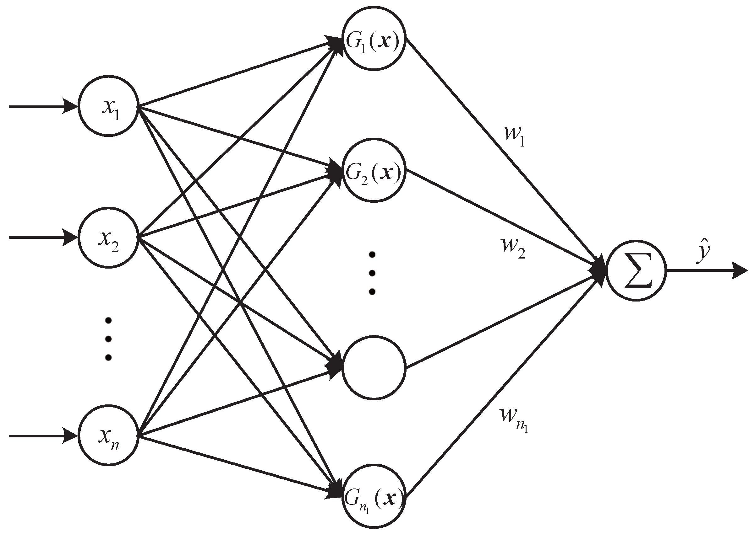
The radial basis function (RBF) NN is a feed-forward NN with only one hidden layer whose structure is demonstrated in Figure 6. The RBFNN has Gaussian functions as its hidden neurons. The GRBFNN is a modified RBFNN and adopts the generalized Gaussian functions as its hidden neurons [43,44].

The output of the GRBFNN can be expressed as [43,44]

$$\begin{array}{c}\hfill \widehat{y}=\sum _{j=1}^{n_1}{w}_j{G}_j(\mathit{x})=\sum _{j=1}^{n_1}{w}_{j}exp\left(-\frac{\parallel \mathit{x}-c_j{\parallel }^{{\tau }_j}}{d_j^{{\tau }_j}}\right),\end{array}$$

(25)

where $n_1$ is the number of hidden neurons, ${\tau }_j$ is the shape parameter of the jth radial basis function in the hidden layer, and $c_j$ and $d_j$ are, respectively, the center and width of the jth radial basis function.

In order to determine the parameters $\mathit{\tau }$, $\mathit{c}$ and $\mathit{d}$ in the hidden layer and the connection weight $w_j$, the aforementioned BP algorithm can also be employed.

4.1.3. Extreme Learning Machine

The ELM is also a feed-forward neural network with only one hidden layer as demonstrated in Figure 6. However, the ELM and GRBFNN have different parameter learning algorithms and different activation functions in the hidden neurons.

In the ELM, the activation functions in the hidden neurons can be the hard-limiting activation function, the Gaussian activation function, the Sigmoidal function, the Sine function, etc. [36,37].

In addition, the learning algorithm for the ELM is listed below:

• Randomly assign input weights or the parameters in the hidden neurons.
• Calculate the hidden layer output matrix $\mathit{H}$, where

  $$\begin{array}{c}\hfill \mathit{H}={\left(\begin{array}{ccc}{G}_1({\mathit{x}}^{(1)})& \cdots & G_{n_1}({\mathit{x}}^{(1)})\\ ⋮& \ddots & ⋮\\ G_1({\mathit{x}}^{(N)})& \cdots & G_{n_1}({\mathit{x}}^{(N)})\end{array}\right)}_{N\times n_1}.\end{array}$$

  (26)
• Calculate the output weights $\mathit{w}={[w_1,w_2,\cdots ,w_{n_1}]}^{\mathtt{T}}={\mathit{H}}^{+}\mathit{Y}$, where $\mathit{Y}={[y^{(1)},y^{(2)},\cdots ,y^{(N)}]}^{\mathtt{T}}$ and ${\mathit{H}}^{+}$ is the Moore–Penrose generalized inverse of the matrix $\mathit{H}$.

This learning process is very fast and can lead to excellent modeling performance. Hence, the ELM has found lots of applications in different research fields.

4.1.4. Support Vector Regression

The SVR is a variant of SVM. It can yield improved generalization performance through minimizing the generalization error bound [45]. In addition, the kernel trick is adopted to realize the nonlinear transformation of input features.

The model of the SVR can be defined by the following function

$$\begin{array}{c}\hfill \widehat{y}=f(\mathit{x},\mathit{w})={\mathit{w}}^{\mathtt{T}}\phi (\mathit{x})+b,\end{array}$$

(27)

where $\mathit{w}=[w_1,\cdots ,w_n]$, $\phi (\mathit{x})$ is the nonlinear mapping function.

Using the training set $\aleph ={\{({\mathit{x}}^{(l)},y^{(l)})\}}_{l=1}^N$, we can determine the parameters $\mathit{w}$ and b, and then obtain the SVR model as

$$\begin{array}{c}\hfill \widehat{y}=f(\mathit{x})=\sum _{l=1}^N{{\mathbf{w}}^{*}}^{\mathtt{T}}\phi (\mathit{x})+b^{*},\end{array}$$

(28)

where

$$\begin{array}{c}\hfill \left\{\begin{array}{cc}\hfill {\mathbf{w}}^{*}& =\sum _{l=1}^N({\alpha }_l^{*}-{\alpha }_l)\phi ({\mathit{x}}^{(l)}),\hfill \\ \hfill b^{*}& =\frac{1}{y_l}-{{\mathbf{w}}^{*}}^{\mathtt{T}}\phi ({\mathit{x}}^{(l)}),\hfill \end{array}\right.\end{array}$$

(29)

in which ${\alpha }_l$ and ${\alpha }_l^{*}$ are the Langrange multipliers and can be determined by solving the following dual optimization problem [46]:

$$\begin{array}{c}\hfill \left\{\begin{array}{c}\underset{\alpha ,{\alpha }^{*}}{max}-\epsilon \sum _{l=1}^N({\alpha }_l^{*}+{\alpha }_l)+\sum _{l=1}^N({\alpha }_l^{*}-{\alpha }_l)y^{(l)}-\frac{1}{2}\sum _{l,t=1}^N({\alpha }_l^{*}-{\alpha }_l)({\alpha }_t^{*}-{\alpha }_t){\phi }^{\mathtt{T}}({\mathit{x}}^{(l)})\phi ({\mathit{x}}^{(t)}),\hfill \\ \sum _{l=1}^N{\alpha }_l^{*}=\sum _{l=1}^N{\alpha }_l,0<{\alpha }_l,{\alpha }_l^{*}<C,\hfill \end{array}\right.\end{array}$$

(30)

where C is the regularization parameter and $\epsilon$ is the error tolerance parameter.

4.2. Applied Data Sets and Experimental Setting

In this subsection, first of all, the building energy consumption data sets will be described. Next, three design factors that are utilized to determine the optimal structure of the MDBN will be shown. Finally, five indices will be given to evaluate the performances of the predictive models.

4.2.1. Applied Data Sets

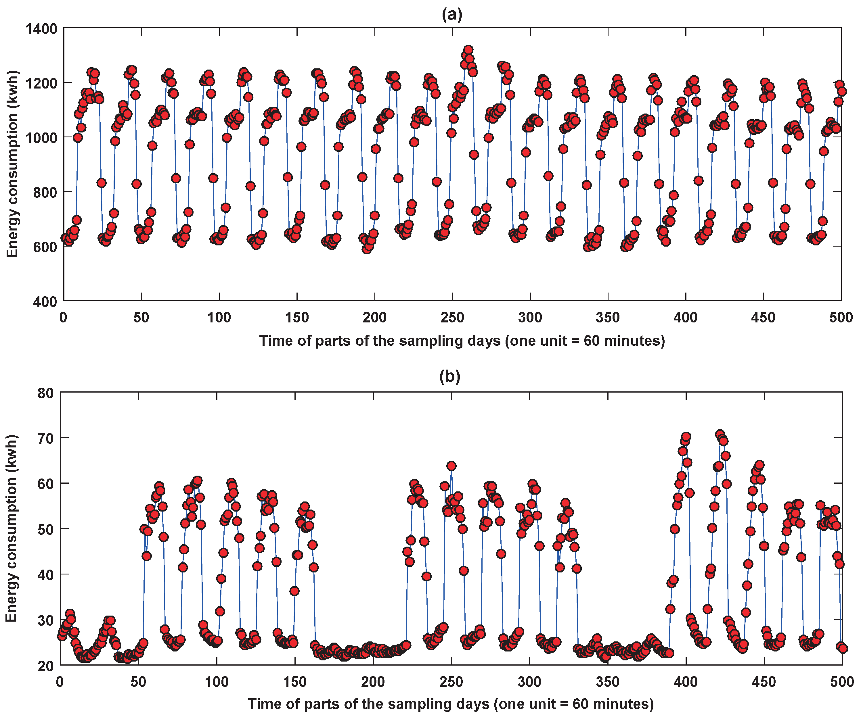
Two kinds of building energy consumption data sets were downloaded from [47]. The first data set includes 34,848 samples from 2 January 2010 to 30 December 2010. The data in this data set were collected every 15 min in one retail store in Fremont, CA, USA. We then aggregated them to generate the hourly energy consumption data. The second data set contains 22,344 samples from 4 April 2009 to 21 October 2011. The data in this set were collected every 60 min in one office building in Fremont, CA, USA. Parts of the samples of the two data sets are depicted in Figure 7.

4.2.2. Design Factors for MDBN

To determine the optimal structure of the MDBN for building energy consumption prediction, we will take three design factors, the number of hidden layers, hidden neurons and input variables, with their corresponding levels into account. The three design factors and their corresponding levels are presented in

Table 1. Design factors and their corresponding levels.

Design Factors	Level
	1	2	3
i	2 hidden layers	3 hidden layers	4 hidden layers
ii	50 hidden units	100 hidden units	150 hidden units
iii	4 input variables	5 input variables	6 input variables

and discussed in detail below.

• Design Factor i: the number of hidden layers k
  The number of hidden layers determines how many RBMs are stacked. In this study, we consider the number of hidden layers 2, 3 and 4 as Levels 1, 2 and 3, respectively.
• Design Factor ii: the number of uth hidden units $n_u$
  The number of hidden units is an important factor that greatly influences the performance of the MDBN model. Here, we assume that the numbers of neurons in all hidden layers are equal, i.e., $n_1=n_2=\cdots =n_k$. In this paper, we set the number of neurons 50, 100 and 150 as Levels 1, 2 and 3, respectively.
• Design Factor iii: the number of input variables r
  In this paper, we utilize r energy consumption data in the building energy consumption time series before time t to predict the value at time t. In other words, we utilize $\mathit{x}=[y(t-1),y(t-2),\dots ,y(t-r)]$ to predict the value of $y=y(t)$. Here, we consider the number of input variables 4, 5 and 6 as Levels 1, 2 and 3, respectively.

4.2.3. Comparison Setting

In this study, the performances of all the predictors constructed by utilizing the energy-consuming patterns are compared with those designed by the original data. To evaluate the performances of the models, we utilize the following two kinds of indices.

We first consider the mean absolute error (MAE), the root mean square error (RMSE), and the mean relative error (MRE), and calculate them as

$$\begin{array}{cc}\hfill MAE& =\frac{1}{K}\sum _{l=1}^K\left|{\widehat{y}}^{(l)}-y^{(l)}\right|,\hfill \end{array}$$

(31)

$$\begin{array}{cc}\hfill RMSE& =\sqrt{\frac{{\sum }_{l=1}^K{({\widehat{y}}^{(l)}-y^{(l)})}^2}{K}},\hfill \end{array}$$

(32)

$$\begin{array}{cc}\hfill MRE& =\frac{1}{K}\sum _{l=1}^K\frac{\left|{\widehat{y}}^{(l)}-y^{(l)}\right|}{y^{(l)}}\times 100\%,\hfill \end{array}$$

(33)

where K is the number of training or testing data pairs, and ${\widehat{y}}^{(l)},y^{(l)}$ are, respectively, the predicted value and actual value with respect to the input ${\mathit{x}}^{(l)}$.

The MAE, RMSE and MRE are common measures of forecasting errors in time series analysis. They serve to aggregate the magnitudes of the prediction errors into a single measure. The MAE is an average of the absolute errors between the predicted values and actual observed values. In addition, the RMSE represents the sample standard deviation of the differences between the predicted values and the actual observed values. As larger errors have a disproportionately large effect on MAE and RMSE, they are sensitive to outliers. The MRE, also known as the mean absolute percentage deviation, can remedy this drawback, and it expresses the prediction accuracy as a percentage through dividing the absolute errors by their corresponding actual values. For prediction applications, the smaller the values of MAE, RMSE and MRE are, the better the forecasting performance will be.

To better show the validity of the models, we also consider another two statistical indices, which are, respectively, the Pearson correlation coefficient, denoted as r, and the coefficient of determination, denoted as $R^2$. These two indices can be calculated as

$$\begin{array}{cc}\hfill r& =\frac{K({\sum }_{l=1}^K{\widehat{y}}^{(l)}·y^{(l)})-({\sum }_{l=1}^K{\widehat{y}}^{(l)})·({\sum }_{l=1}^K{y}^{(l)})}{\sqrt{(K{\sum }_{l=1}^K{({\widehat{y}}^{(l)})}^2-{({\sum }_{l=1}^K{\widehat{y}}^{(l)})}^2)·(K{\sum }_{l=1}^K{(y^{(l)})}^2-{({\sum }_{l=1}^K{y}^{(l)})}^2)}},\hfill \end{array}$$

(34)

$$\begin{array}{cc}\hfill R^2& =\frac{{\left[{\sum }_{l=1}^K({\widehat{y}}^{(l)}-{\widehat{y}}_{Ave})·(y^{(l)}-y_{Ave})\right]}^2}{{\sum }_{l=1}^K({\widehat{y}}^{(l)}-{\widehat{y}}_{Ave})·{\sum }_{l=1}^K(y^{(l)}-y_{Ave})},\hfill \end{array}$$

(35)

where K is also the number of training or testing data pairs, and ${\widehat{y}}_{Ave}$, $y_{Ave}$ are, respectively, the averages of the predicted and actual values.

The statistic r is a measure of the linear correlation between the actual values and the predicted values. It ranges from $-1$ to 1, where $-1$ means the total negative linear correlation, while 1 is total positive linear correlation. The statistic $R^2$ provides a measure of how well actual observed values are replicated by the predicted values. In other words, it is a measure of how good a predictor might be constructed from the observed training data [48]. The value of $R^2$ ranges from 0 to 1. In regression applications, the larger the values of r and $R^2$ are, the better the prediction performances will be.

4.3. Energy Consumption Prediction for the Retail Store

In this subsection, the energy-consuming pattern of the retail store will be extracted from the retail store data set firstly. Then, the configurations of the five prediction models for predicting the retail store energy consumption will be shown in detail. At last, the experimental results will be given.

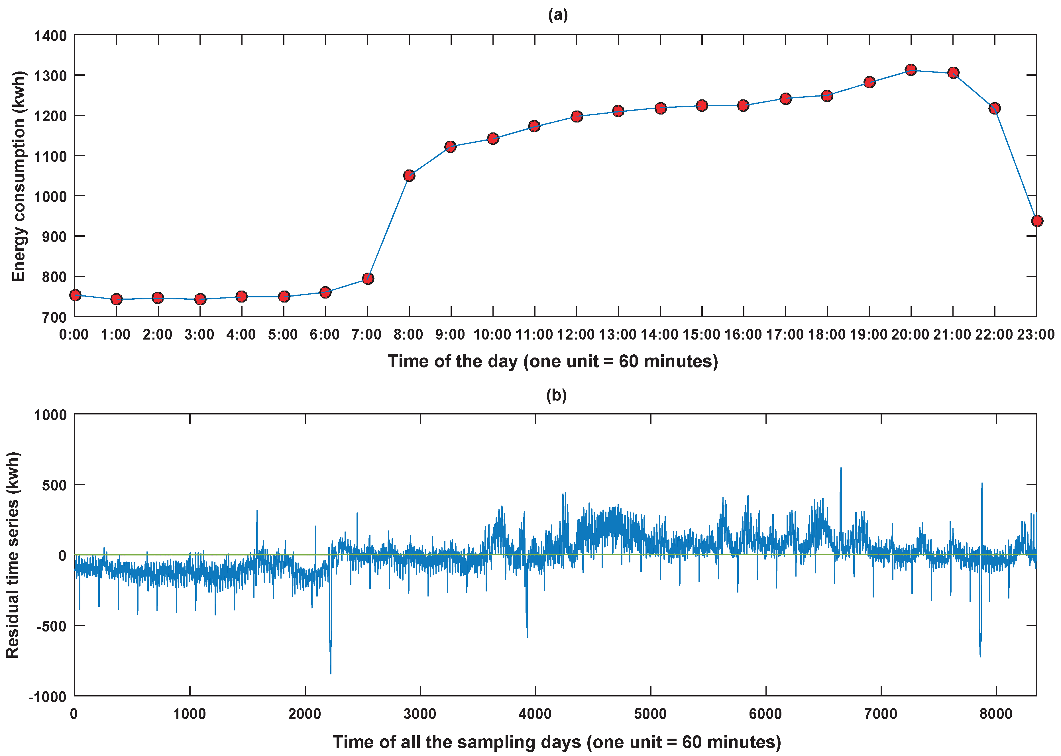
4.3.1. Energy-Consuming Pattern of the Retail Store

We utilize Equations (6) and (7) to obtain the daily-periodic energy-consuming pattern and the residual time series of the retail store.

Figure 8a shows the daily-periodic energy-consuming pattern. In addition, the residual time series of the retail store, which is used to optimize the MDBN is demonstrated in Figure 8b.

4.3.2. Configurations of the Prediction Models

As aforementioned, we will take three design factors, the number of hidden layers, hidden neurons and input variables, with their corresponding levels into account to determine the optimal structure of the MDBN model for building energy consumption prediction. Consequently, $3^3=27$ trials are ran. In addition, the experimental results are shown in

Table 2. Experimental results of the MDBN in 27 trails under the consideration of three design factors and their corresponding levels.

Trails	Factor			Residual Data			Trails	Factor			Residual Data
	i	ii	iii	MAE (kwh)	MRE (%)	RMSE (kwh)		i	ii	iii	MAE (kwh)	MRE (%)	RMSE (kwh)
1	1	1	1	49.21	5.26	80.79	15	2	2	3	49.65	5.31	80.03
2	1	1	2	48.74	5.18	80.03	16	2	3	1	50.18	5.36	82.13
3	1	1	3	48.73	5.19	78.06	17	2	3	2	48.43	5.11	78.24
4	1	2	1	49.12	5.24	81.20	18	2	3	3	48.33	5.12	77.96
5	1	2	2	48.25	5.16	79.39	19	3	1	1	47.71	5.03	76.83
6	1	2	3	49.16	5.24	79.36	20	3	1	2	48.37	5.11	77.63
7	1	3	1	49.42	5.28	81.85	21	3	1	3	48.13	5.11	77.60
8	1	3	2	49.33	5.25	81.40	22	3	2	1	48.72	5.18	79.16
9	1	3	3	48.65	5.18	78.69	23	3	2	2	49.66	5.28	79.84
10	2	1	1	48.73	5.20	79.65	24	3	2	3	49.08	5.22	78.03
11	2	1	2	49.61	5.29	81.24	25	3	3	1	51.07	5.50	83.35
12	2	1	3	47.95	5.08	77.96	26	3	3	2	48.81	5.18	79.22
13	2	2	1	48.83	5.17	79.93	27	3	3	3	48.33	5.09	77.50
14	2	2	2	49.97	5.33	81.33

. It is obvious that trail 19 can obtain the best performance. In other words, the optimal structure of the MDBN for retail store energy consumption prediction has four hidden layers, 150 hidden units and four input variables.

Furthermore, the parameter configurations of the other four comparative predictors for retail store energy consumption prediction are listed in detail as follows.

• For the BPNN, there were 110 neurons in the hidden layer that can realize the nonlinear transformation of features by the sigmoid function. Additionally, the algorithm was ran for 7000 iterations to achieve the learning objective.
• For the GRBFNN, the 6-fold cross-validation was adopted to determine the optimized spread of the radial basis function. Furthermore, the spread was chosen from 0.01 to 2 with the 0.1 step length.
• For the ELM, there were 100 neurons in the hidden layer, and the hardlim function was chosen as the activation function for converting the original features into another space.
• For the SVR, the penalty coefficient was set to be 80, and the radial basis function was chosen as the kernel function to realize the nonlinear transformation of input features.

4.3.3. Experimental Results

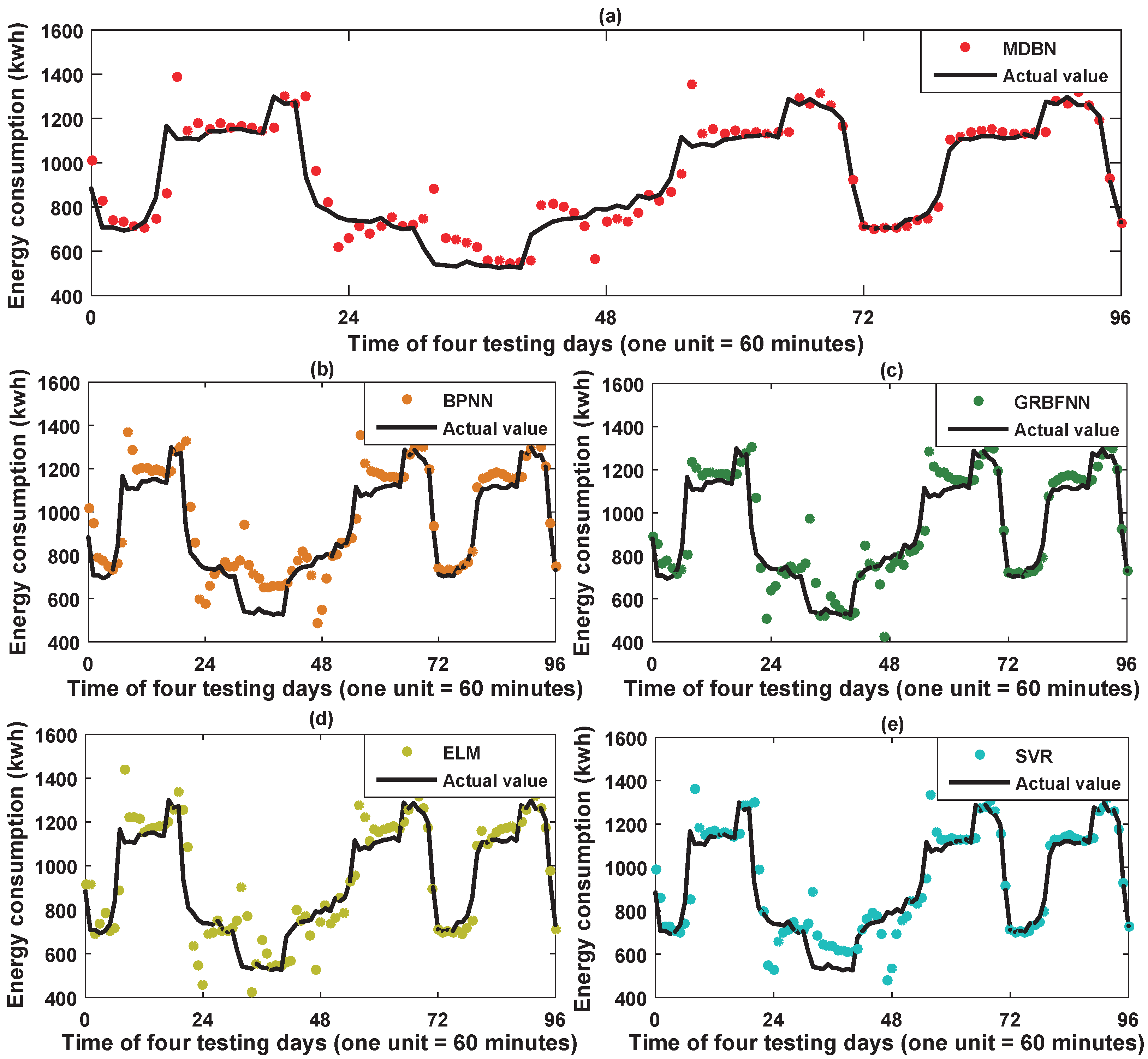
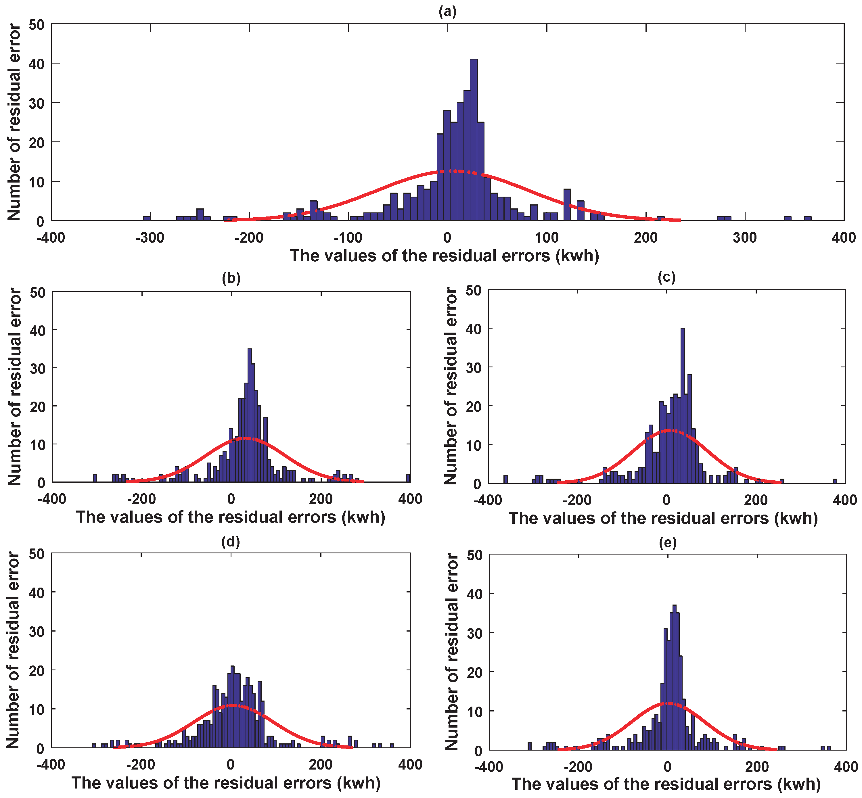
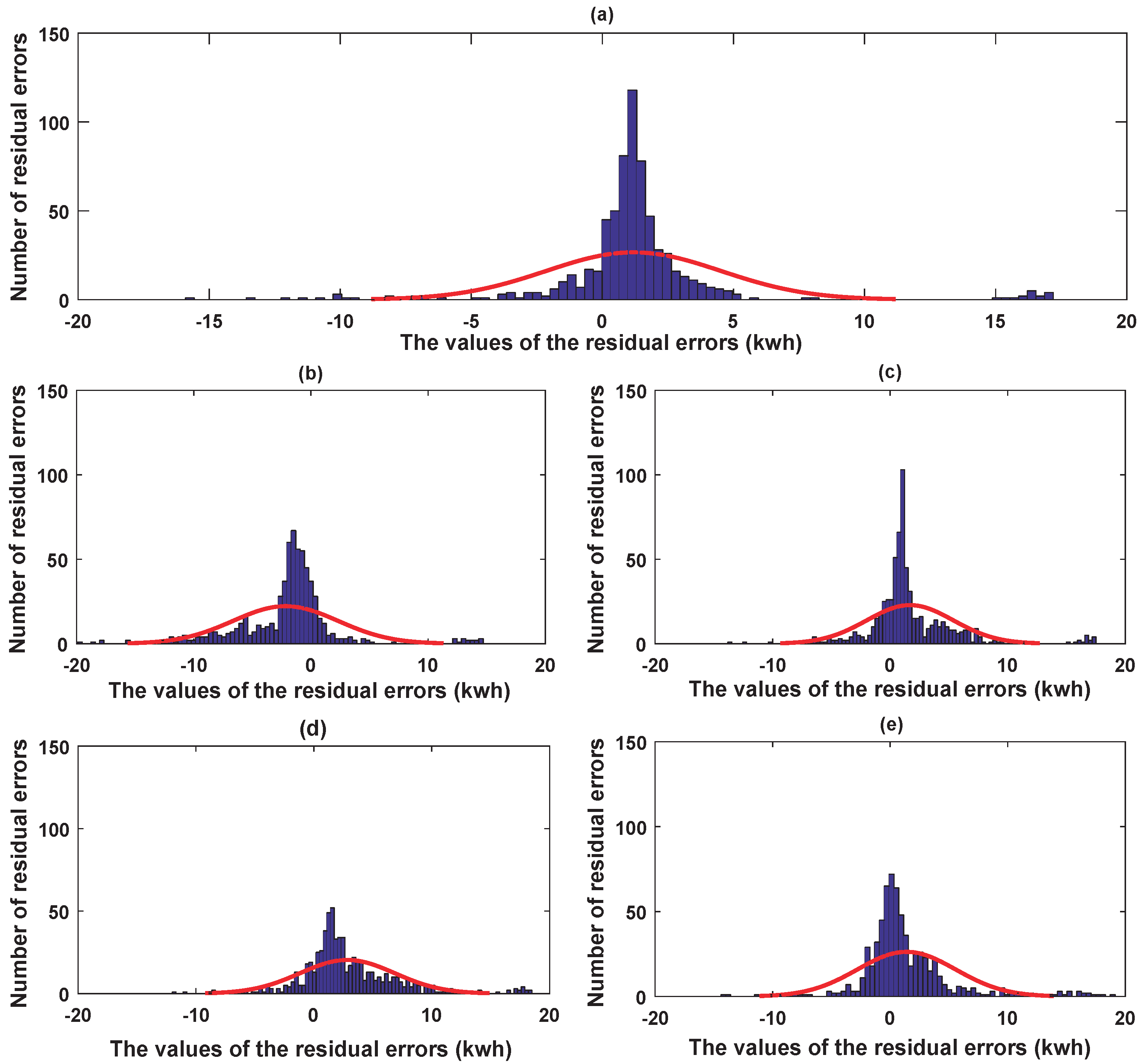
For the testing data of the retail store, parts of the prediction results of the five predictors constructed by utilizing the energy-consuming pattern are illustrated in Figure 9. Furthermore, for better visualization, the prediction error histograms of the five predictors are shown in Figure 10. It is obvious that the more the prediction errors float around zero, the better the forecasting performance of the predictor will be.

Then, to examine the superiority of the hybrid model for the retail store energy consumption prediction, the five prediction models are compared considering different data types (the original and residual data). The original data means that the predictors are learned using the original data series, while the residual data means that the predictors are constructed by both the energy-consuming pattern and the residual data series. Experimental results are demonstrated in detail in

Table 3. The performances of the five models for the retail store energy consumption prediction.

Methods	Data Type	MAE (kwh)	MRE (%)	RMSE (kwh)	r	${\mathit{R}}^2$
MDBN	Residual data	47.71	5.03	76.83	0.94	0.89
	Original data	54.38	5.59	86.43	0.93	0.86
BPNN	Residual data	65.69	7.24	93.38	0.92	0.85
	Original data	75.45	8.20	100.40	0.94	0.87
GRBFNN	Residual data	54.60	5.75	83.87	0.93	0.87
	Original data	52.51	5.62	87.54	0.93	0.86
ELM	Residual data	58.54	6.29	88.62	0.93	0.86
	Original data	78.86	8.34	113.02	0.89	0.79
SVR	Residual data	48.28	5.19	81.31	0.93	0.87
	Original data	52.19	5.42	89.93	0.92	0.85

.

4.4. Energy Consumption Prediction for the Office Building

In this subsection, first of all, the energy-consuming pattern of the office building will be extracted from the office building data set. Then, the configurations of the five prediction models for predicting the office building energy consumption will be shown in detail. Finally, the experimental results will be given.

4.4.1. Energy-Consuming Pattern of the Office Building

Being similar to the retail store experiment, we utilize Equations (8)–(14) to obtain the weekly-periodic energy-consuming pattern and the residual time series of the office building.

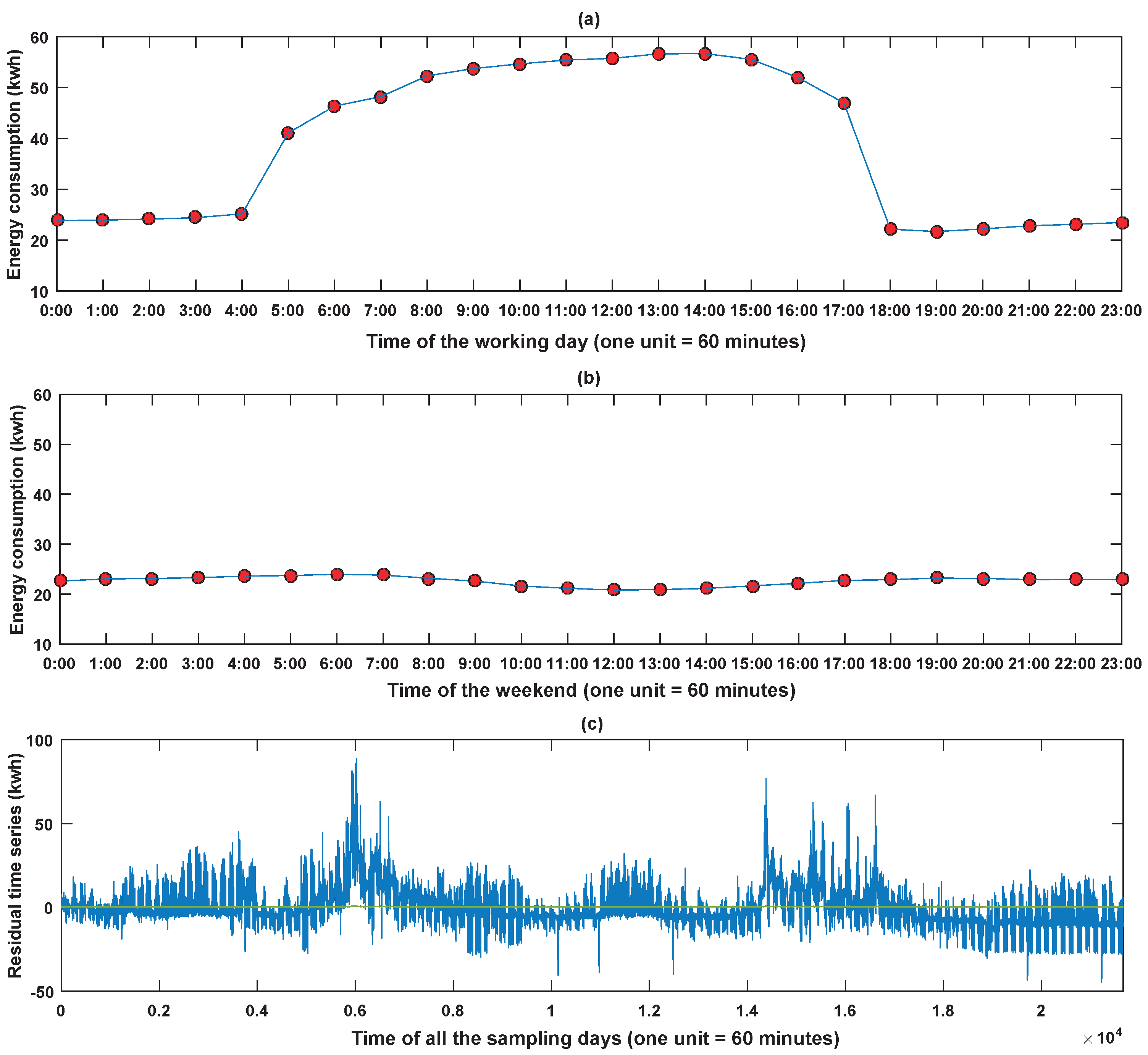
As mentioned previously, the weekly-periodic energy-consuming pattern should include two parts, which are the weekday pattern and the weekend pattern. The obtained weekday pattern is depicted in Figure 11a, while the weekend pattern is shown in Figure 11b. We can observe that the energy consumption in weekends is quite different from that in weekdays. After removing the energy-consuming pattern, the residual time series of the office building is demonstrated in Figure 11c. This residual time series is utilized to train the MDBN in the hybrid model.

4.4.2. Configurations of the Prediction Models

Similarly, we run $3^3=27$ trials to determine the optimal structure of the MDBN model for the office building energy consumption prediction. The experimental results are listed in

Table 4. Experimental results of the MDBN in 27 trails under the consideration of three design factors and their corresponding levels.

Trails	Factor			Residual Data			Trails	Factor			Residual Data
	i	ii	iii	MAE (kwh)	MRE (%)	RMSE (kwh)		i	ii	iii	MAE (kwh)	MRE (%)	RMSE (kwh)
1	1	1	1	2.30	12.67	3.69	15	2	2	3	2.35	12.99	3.69
2	1	1	2	2.22	12.29	3.61	16	2	3	1	2.25	12.49	3.65
3	1	1	3	2.32	12.74	3.67	17	2	3	2	2.30	12.78	3.68
4	1	2	1	2.23	11.97	3.63	18	2	3	3	2.36	13.10	3.71
5	1	2	2	2.35	12.81	3.71	19	3	1	1	2.21	12.19	3.65
6	1	2	3	2.40	13.10	3.71	20	3	1	2	2.23	12.29	3.66
7	1	3	1	2.17	11.93	3.58	21	3	1	3	2.27	12.54	3.67
8	1	3	2	2.29	12.70	3.67	22	3	2	1	2.17	12.06	3.60
9	1	3	3	2.27	12.55	3.63	23	3	2	2	2.26	12.51	3.65
10	2	1	1	2.26	12.53	3.65	24	3	2	3	2.23	12.25	3.67
11	2	1	2	2.31	12.83	3.68	25	3	3	1	2.14	11.91	3.60
12	2	1	3	2.36	13.10	3.70	26	3	3	2	2.32	12.64	3.73
13	2	2	1	2.09	11.62	3.54	27	3	3	3	2.21	12.30	3.64
14	2	2	2	2.31	12.84	3.68

. As shown in Table 4, the trail 13 obtains the best performance. Consequently, the optimal structure of the MDBN in the hybrid model for office building has three hidden layers, 100 hidden units in each layer and four input variables.

For the other four comparative predictors, their parameter configurations for the office building energy consumption prediction are listed as follows:

• For the BPNN, there were 200 neurons in the hidden layer. Furthermore, the sigmoid function was chosen to realize the nonlinear transformation of features. Additionally, we ran the BP algorithm 1000 times to obtain the final outputs.
• For the GRBFNN, the 5-fold cross-validation was utilized to determine the optimized spread of the radial basis function. Furthermore, the spread was chosen from 0.01 to 2 with a 0.1 step length.
• For the ELM, there were 150 neurons in the hidden layer, and the hardlim function was chosen as the activation function for converting the original features into another space.
• For the SVR, the penalty coefficient was set to be 10 and the sigmoid function was chosen as the kernel function to realize the nonlinear transformation of input features.

4.4.3. Experimental Results

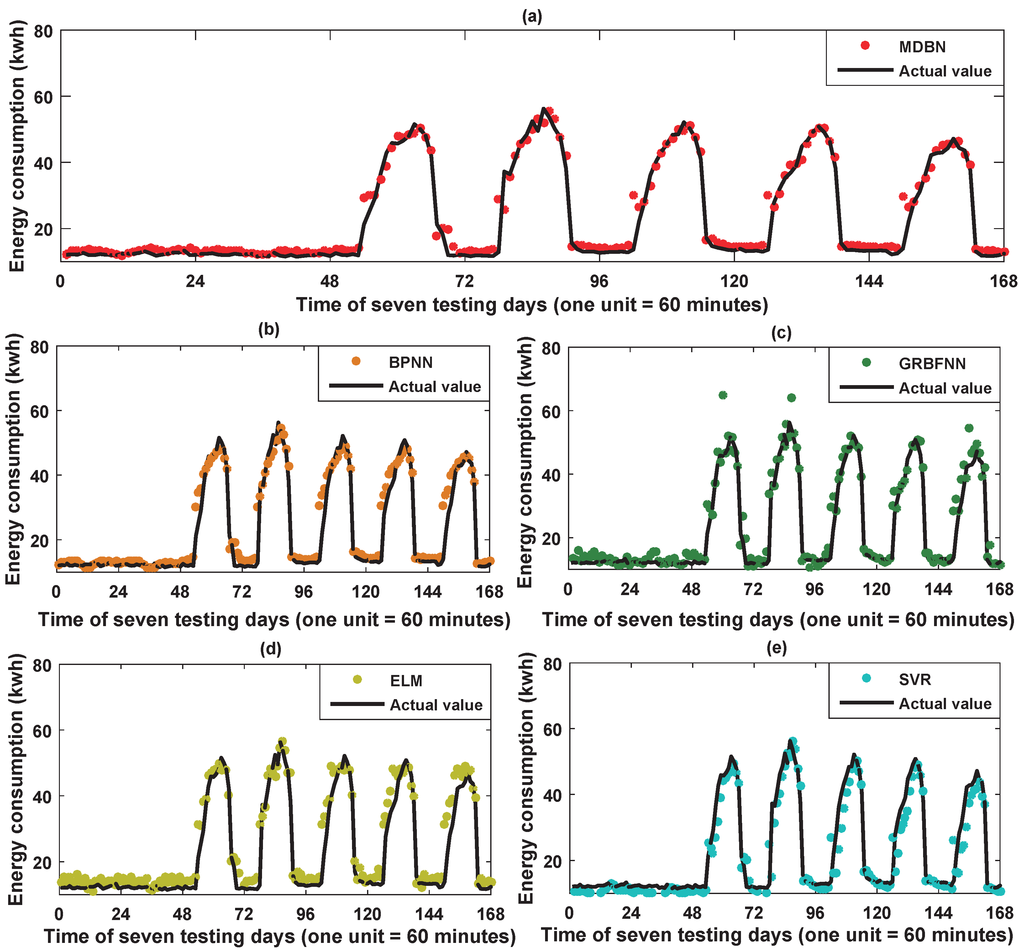
For the testing data of the office building, parts of the prediction results of the five predictors are illustrated in Figure 12. Again, for better visualization, the prediction error histograms of the five predictors are shown in Figure 13.

Then, in order to examine the superiority of the hybrid model for the office building energy consumption prediction, the five prediction models are compared under the consideration of different data types (the original and residual data). Experimental results are demonstrated in

Table 5. The performances of the five models with different data types for the office building energy consumption prediction.

Methods	Data Type	MAE (kwh)	MRE (%)	RMSE (kwh)	r	${\mathit{R}}^2$
MDBN	Residual data	2.09	11.62	3.54	0.97	0.93
	Original data	2.32	11.50	4.19	0.95	0.90
BPNN	Residual data	2.57	12.64	4.04	0.96	0.93
	Original data	3.85	23.21	4.75	0.95	0.91
GRBFNN	Residual data	2.54	12.62	4.39	0.95	0.91
	Original data	4.35	21.94	5.98	0.93	0.87
ELM	Residual data	3.50	17.18	4.92	0.96	0.92
	Original data	4.61	25.52	5.92	0.90	0.82
SVR	Residual data	3.23	14.89	4.98	0.94	0.88
	Original data	6.13	34.42	7.55	0.92	0.85

.

4.5. Comparisons and Discussions

As discussed previously, smaller values of the MAE, RMSE and MRE represent better prediction results while lager values of r and $R^2$ correspond to better performance. Considering all the values of such indices as shown in Table 3 and Table 5 (It is worth noting that the values of the indices in Table 3 are about the retail energy consumption while the values in Table 5 are about the office energy consumption. The retail building consumed much more energies than the office building. As a result, some values of the MAE, RMSE and MRE in Table 3 are larger than those in Table 5), the predictors constructed by utilizing the energy-consuming patterns perform better than those designed only by the original data. Taking the RMSE index for example, in the first experiment, the accuracies of the MDBN, BPNN, GRBFNN, ELM and SVR based hybrid models are promoted by 11.1%, 7.0%, 4.2%, 21.6% and 9.6%, respectively, while, in the second experiment, the accuracy improvements of such models are 15.6%, 14.8%, 26.5%, 16.9% and 34.0%, respectively. As a result, we can draw a conclusion that the periodicity knowledge is helpful to improve the accuracy for building energy consumption prediction.

From Figure 9 and Figure 12, we can see that the hybrid DBN model can not only predict the regular testing data well for both the retail store and the office building energy consumption from the global perspective, but also give the best prediction results for the noisy irregular data, e.g., the sampling points from 25 to 50 in Figure 9 in the retail store experiment. These irregular testing data can reflect the uncertainties in the energy consumption time series. In other words, the proposed hybrid DBN model has the most powerful ability to deal with the uncertain and/or the randomness in the historical building energy consumption data.

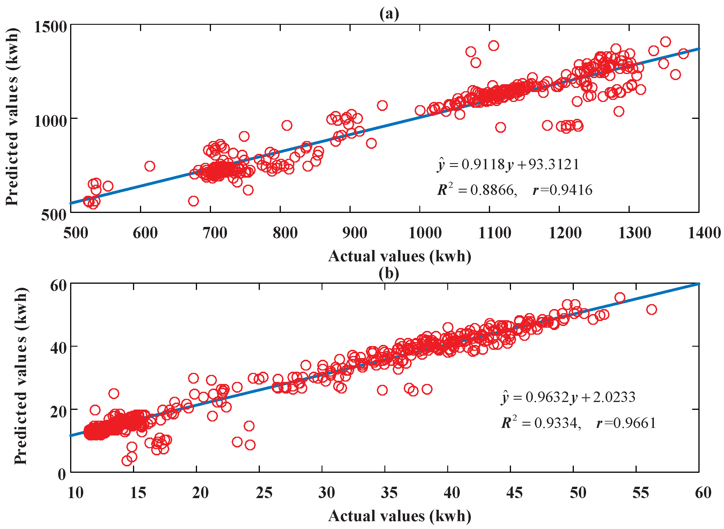
Figure 10 and Figure 13 demonstrated the prediction error histograms of the five models designed through using the periodicity knowledge in the two experiments. In the histograms, the horizontal direction depicts the exact values of the prediction errors, while the vertical direction indicates the number of the prediction errors in different partitioned intervals. The more the prediction errors float around zero, the better performance the predictors will achieve. From both figures, we can clearly observe that the proposed hybrid DBN model has more prediction errors floating near zero compared with the other four artificial intelligence techniques—that is to say, the approximation capability of the proposed hybrid DBN model is promising for the two experimented buildings. Furthermore, to further validate the accuracy of the MDBN based hybrid model, scatter plots of the actual and predicted values in the two experiments are demonstrated in Figure 14a,b, respectively. From Figure 14, we can observe that the predicted values from the hybrid DBN model can duplicate the actual values well.

Among all the predictors constructed by both the original and residual data, the proposed MDBN based hybrid model has the best prediction accuracy in the two experiments as shown in Table 3 and Table 5. This phenomenon indicates that the proposed deep learning method has the miraculous learning and prediction abilities in time series forecasting applications. This also verifies the powerful feature extraction ability of the deep learning algorithm and the effectiveness of the modified learning strategies.

One thing to be mentioned is that the numbers of the data used in this paper are not very big (about the ten thousand scale). Even though the hybrid MDBN model is not learned by big data in both experiments, it still shows us excellent performances. This is also consistent with some other application results where the DBNs were trained without a mass of data. For example, in [49,50], the DBNs were applied to the time series prediction and the wind power prediction, which also do not have a large quantity of data. In both applications, the experimental results demonstrated that the DBN approach performs best compared with the traditional techniques. All these applications verified the learning ability of the DBN models for not very large data applications.

5. Conclusions

As is well known, many kinds of time series data, e.g., the traffic flow time series and the electricity consumption time series, have the periodicity property. The hybrid model can be expected to yield better performance in the predictions of such time series. In the future, we will extend our approach to these applications. On the other aspect, our study only focuses on the data science that tries to utilize the data to realize the energy-consumption prediction without considering any scientific or practical information of energy related principles. Theoretically, the energy related principles are very helpful to improve the prediction performance. We are now exploring the strategies to construct the novel hybrid prediction models through combining the energy related principles and observed data to further improve the prediction accuracy.

In this paper, a hybrid model is presented to further improve the prediction accuracy for building energy consumption prediction. The proposed model combines the MDBN model with the periodicity knowledge to obtain the final prediction results. The theoretical contributions of this study consist of two aspects: (1) the periodicity knowledge was extracted and encoded into the prediction model. In addition, the prediction accuracy can be greatly improved through utilizing this kind of prior knowledge; (2) a novel learning algorithm that combines the contrastive divergence algorithm and the least squares method was proposed to optimize the parameters of the MDBN. This is the first time that the DBN is applied to the building energy consumption prediction. On the other hand, this study applied the proposed approach to the energy consumption prediction of two kinds of buildings. Experimental and comparison results verified the effectiveness and superiorities of the proposed hybrid model.

References