Bond Graph Simulation of Error Propagation in Position Estimation of a Hydraulic Cylinder Using Low Cost Accelerometers


Department of Fluid Mechanics, LABSON, Technical University of Catalonia, Colom 7, 08222 Terrassa, Spain
*
Author to whom correspondence should be addressed.
Energies 2018, 11(10), 2603; https://doi.org/10.3390/en11102603
Submission received: 2 September 2018
/
Revised: 22 September 2018
/
Accepted: 25 September 2018
/
Published: 29 September 2018
(This article belongs to the Special Issue Energy Efficiency and Controllability of Fluid Power Systems 2018)
Abstract
:The indirect calculation from acceleration of transversal displacement of the piston inside the body of a double effect linear hydraulic cylinder during its operating cycle is assessed. Currently an extensive effort exists in the improvement of the mechanical and electronic design of the highly sophisticated MEMS accelerometers. Nevertheless, the predictable presence of measurement errors in the current commercial accelerometers is the main origin of velocity and displacement measurement deviations during integration of the acceleration. A bond graph numerical simulation model of the electromechanical system has been developed in order to forecast the effect of several measurement errors in the use of low cost two axes accelerometers. The level of influence is assessed using quality indicators and visual signal evaluation, for both simulations and experimental results. The obtained displacements results are highly influenced by the diverse dynamic characteristics of each measuring axis. The small measuring errors of a simulated extremely high performance sensor generate only moderate effects in longitudinal displacement but deep deviations in the reconstruction of piston transversal movements. The bias error has been identified as the source of the higher deviations of displacement results; although, its consequences can be easily corrected.
1. Introduction
1.1. Research Overview
At present, acceleration measurements are obtained with considerable simplicity due to the small size, low cost and adaptability of the currently available acceleration sensors. In consequence, high interest exists in various fields of engineering to use these indirect measures to obtain velocity and displacement values, which would be expensive to obtain by direct measurement means. Furthermore, this type of measure would be very useful in situations where fixed points of reference are difficult to establish or unavailable. It would be the case of measurement systems like LASERs or linear variation differential transformers (LVDTs).
The velocity and the position are easily calculated from the acceleration by means of successive integrations, that is:
where v(t) is the velocity, a(t) is the acceleration and x(t) displacement at time t, so, assuming that both initial displacement and velocity are known, the position and velocity of an object would be obtained at any time from the measurement of the acceleration.
This strategy of indirect measurement of displacement has been exploited in several fields of engineering. For example, Moschas et al. [1] studied the use of accelerometers in monitoring the displacement of a high-rise bridge. Thus, an algorithm was developed to obtain the initial conditions of position and velocity. In case both velocity and position aren’t zero at the time of integration it’s concluded that a large displacement measuring error will be generated.
On the other hand, accelerometers have been widely used to reconstruct the position and velocity of displacement of certain structures during earthquakes. Even in short periods of time, the obtained measurements show a drift of up to one meter in comparison with direct measurements of displacement by Global Positioning System (GPS) [1]. This drift is the result of the measurement device error propagation and the sampling time instability, among others, during the double integration process. It should be noted that the study determines that the measurement error of the acceleration is magnified at the bottom and end of the sensor measurement scale.
The estimation of velocity and position is also necessary for the proportional-integral-derivative (PID) control of mechanical devices [2]. The existence of noise in both low and high frequencies would cause a drift in the velocity and position reconstruction process. In this particular case, a spectral noise subtraction method is developed from the signal of the resting periods.
As can be seen, the literature in general shows the existence of multiple error sources. Consequently, the presented Equations (1) and (2) don’t allow an accurate calculation of real velocity and displacement from acceleration. Stiros [3] demonstrated, by applying error propagation theory, that the velocity measurement error is a function of the measurement errors of the accelerometer and the duration of the signal; moreover, the displacement error is a function of the square of the duration of the analyzed signal. In particular for acceleration measurements, the main sources of error could be summarized as:
- Non-linearity
- Noise
- Bias: like the two previous measurement errors, t is a deviation from the ideal linearity, common in measurement equipment.
- Signal saturation, which could happen both in the sensor itself and the signal recorder.
- Inadequate bandwidth. Like the signal saturation, it’s a typical error associated with inappropriate selection of the measurement equipment range. Usually, it’s due to the a priori ignorance of the shape of the vibration signal to be measured, which is defined by the frequencies and amplitudes of the involved harmonic signals.
- Cross-axis sensitivity, where the signal measured on one axis affects the measurement of the other axis [4]. Be noticed that it also exist in uniaxial accelerometers, where any transversal acceleration affects the output signal of the main measurement axis.
- Integration method. The usual numerical integration methods, such as the Trapeze or Simpson rules, calculate averages of the registered discrete signals. Thus, they are performing a filtering that minimizes the maximums and maximizes the minimums [5].
- Aliasing: typical during the sampling of continuous signals, it’s reduced by increasing the sampling time [6].
- Analog-to-digital conversion [7].
- Unstable sampling frequency.
- Temperature drifts: to be taken into account particularly in long periods of operation.
- Lack of knowledge of the initial conditions: being a significant issue in some applications as inertial navigation, it’s ruled out when starting from a resting state.
In our previous work, the 3D movement of a piston inside a hydraulic cylinder during cushioning were assessed thanks to an Eddy current displacement sensor [8]. Unfortunately, these sensors are costly and have a limited measurement range and difficult installation. The objective of this paper is to evaluate the feasibility of an alternative measurement system. Specifically, the reconstruction of piston displacement in this particular mechanical system is performed by means of double integration of the measured acceleration. In consequence, the propagation of the errors during the double integration of acceleration has been modeled in a multidomain bond graph numerical simulation model. Finally, the modeling results have been correlated with experimental measurements obtained with a low cost commercial accelerometer.
This paper is organized as follows: Section 1 presents the state of the art and the introduction of the carried out work in this paper. Section 2 details the developed simulation model and the main simulation results obtained. Section 3 describes the main results of the experimental investigation, depending on the measurement axis, and a correlation with the previous simulation results is performed. Finally, in Section 4, conclusions about the feasibility of the indirect measurement of velocity and displacement in the studied application are presented.
1.2. Accelerometers Fundamentals
Given the essential dynamic nature of the acceleration measurement, multiple measurement errors have their origin in the dynamic characteristics of the measurement devices. In other words, the dynamic response of the sensor will result in a certain distortion in the characteristics of phase and amplitude of the obtained measurements field.
Nowadays, thanks to thin-film micromachining technologies, many of the commercial accelerometers are microelectromechanical systems (MEMS) integrated with the necessary control electronics. Usually their integrated circuits are complementary metal-oxide-semiconductor (CMOS)-type [9]. Most accelerometers operate by detecting the force exerted on a mass by an elastic imitation. It means that it’s possible to obtain the magnitude of the acceleration by the displacement x of the mass. Commonly, MEMS accelerometers are based on a capacitive measurement system as a mass-sensitive element. The relative distance of the plates of a differential capacitor, under a reference voltage VR, is affected in response to the acceleration as detailed in Figure 1.
The differential equation of mass displacement x as a function of the external force Fext is obtained from Newton’s law:
where b is the damping coefficient and k is the elastic constant of the spring. As will be exposed later, is considered that when x ≈ 0, Felect ≈ 0. Thus this system can be modeled as a second order transfer function, as follows:
being the canonical equation describing a second-order transfer function as:
So:
where the gain A, natural frequency of the system ωn and damping coefficient ξ are defined as:
In practice, an accelerometer is a capacitive electromechanical system that measures the displacement of the mass as a result of the acceleration experienced and transforms it into an electrical signal. In general, an electronic demodulator is used for this purpose, which typically contains a signal amplifier, an inverter and a low pass filter. Thus, an ideal demodulator can be characterized by a displacement-to-voltage signal linear conversion coefficient Kv.
In fact, these capacitive measurement systems, commonly known as open loop, have several non-linearity sources. Their effect is more important for large displacements of the mass; this happens because the damping coefficient and the electrostatic force change with respect to the third and second power of the displacement, respectively. Although the demodulator design is able to limit this effect to a certain extent, a great limitation on its frequency response, measurement range and bandwidth is generated [10]. This problem is usually solved by implementing a closed-loop control (i.e., PID, as shown in Figure 2); the voltage on the differential capacitance is controlled to generate an electrostatic force contrary to the movement in order to constrain the displacement of the mass. This control can be carried out analogically or, more commonly, digitally [11].
Inevitably, a certain degree of noise exists in the measurement of the accelerometer. The minuscule mass of the sensor creates a problem during the design of high sensitivity accelerometers. The small mass dynamics are affected by the agitation of the molecules of air at the molecular level that exists around it; it’s known as Brownian movement. This noise can be reduced by increasing the mass (option very limited by the manufacturing processes of the MEMS) or by reducing the damping factor, for instance by making the vacuum. Besides, there are other significant noise sources as consequence of the thermal noise in the capacitors of the amplification circuit, the residual movement of the mass or the signal processing in the digital control loop, due to the presence of a dead band of measurement. An accurate design and dimensioning of the electronic circuit as well as the use of signal filters minimize these sources of error [9].
The large number of academic works in this field indicates a great interest in the development of acceleration measurement systems with the best operational behavior. Therefore, the influence of the dimensional and constructive parameters of the capacitance and mass-spring set of the accelerometer [13,14] is studied, as well as the design and sizing of the electronic circuit and the control and modulation strategy of the closed loop control [15,16,17,18,19,20]. In all these cases, the main goal is the reduction of the different error sources that have been listed above (noise, non-linearity, frequency response, thermal drift, bias, cross-axis sensitivity, etc.).
Multiple correction methods have been developed in order to obtain accurate velocity and acceleration curves. An usual strategy for noise suppression is the use of some filters incorporated in the transfer function for the reconstruction of displacement from the acceleration in the frequency domain [21,22,23,24]. Thenozhi [2] proposed a method for the cancellation of decentering (Bias) by adjusting the baseline of the acceleration data. Boore [7] proposed a method of suppression of Analog to Digital Conversion (ADC) error by dithering technique (adding a small random noise signal). Zhu [23] combined the direct measurement of an encoder for position estimation with the use of an accelerometer. So, the author establishes an adaptive mechanism for estimating the gain of the accelerometer during the velocity calculation.
In spite of the extensive bibliography existing in this field, a universal error suppression method apparently doesn’t exist. The applicability of a correction method would depend on the characteristics of the studied system as well as the measuring equipment errors. The case of study affects in its amplitude, spatial axes and frequency modes of the registered movements, the initial conditions and the presence or absence of final displacement. The measurement chain affects in the generated noise, the measurement errors (non-linearity, hysteresis, bias, etc.) or the interaction between measurement axes (cross-axis sensitivity).
Recently, Arias-Lara and De la Colina [25] compared different correction methods, considered by the authors of universal application, under conditions of use related with civil engineering. Each studied method is a specific combination of baseline correction, low/high pass filters and forcing the displacement to zero at the end of the data sample; they are performed in a variable number of steps, with or without iterative calculations. The study offers a guide to select an applicable method depending on the functional conditions, such as the magnitude of the displacement or final displacement existence. Besides, it’s concluded that the excitation frequency doesn’t affect significantly the results.
2. Bond Graph Simulation
2.1. Simulation Model
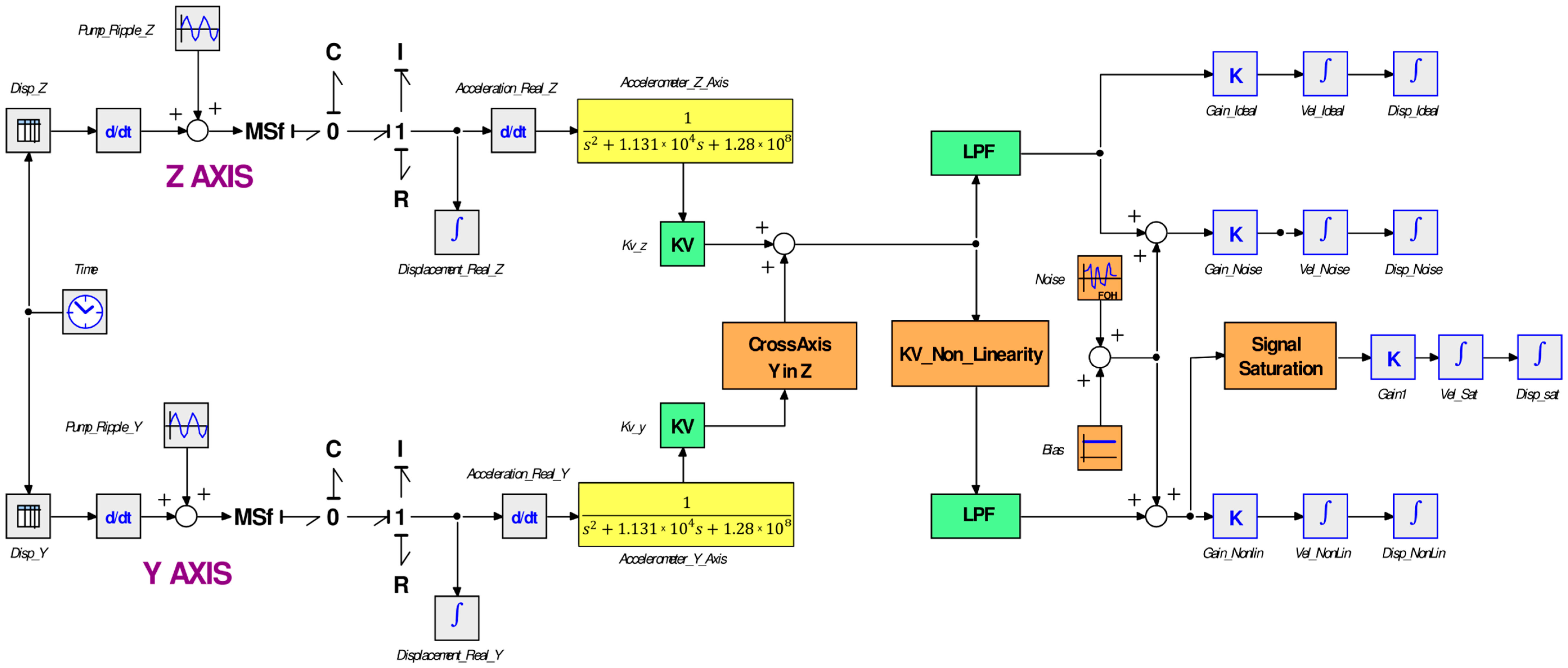
In order to simulate the behavior of a multiaxial accelerometer a bond graph model has been constructed as shown in Figure 3 and Figure 4. With the aim of simplicity, only Z and Y axis are considered, being X axis measurements neglected. The model starts from two displacement sources (Disp_Z and Disp_Y) constructed from previous experimental direct measurements, as shown in Figure 5. The displacements are corresponding with typical piston movements registered in a double effect linear hydraulic cylinder during an operating cycle; the Z axis displacement is related with the extension and retraction way of the cylinder and the Y axis displacement is the transversal movement of the piston inside the cylinder barrel. It should be noted that, the nature of both displacements are very different, where Y axis displacement is several orders of magnitude lower that Z axis displacement. Further description of the operational cycle of the studied hydraulic cylinder and its displacements can be found in our previous experimental work [8]. The generated irregularities in the displacement by the gear pump (Pump_Ripple), as a consequence of the transmitted vibrations and pressure pulses over the piston, are simulated adding a sinusoidal signal into the main displacement value. After deriving the displacement for obtaining the velocity, this complex signal is finally converted into a modular flow source (MSf) in the bond graph model.
The piston affected by the velocity sources (separated in the two independent axes) is represented as a Mass-Spring-Resistance (C, I and R) group experimenting a resulting displacement and acceleration (Real). Attached to the piston mass exists a dual-axis accelerometer represented by a second order transfer function as described in Equation (6).
The considered parameters for the accelerometer model are described in the Table 1. They are based in a low cost commercial MEMS accelerometer as the model ADXL335 by Analog Devices® (Norwood, MA, USA), used later in the experimental work. This accelerometer simulation model shows a perfect linearity and a frequency response, as presented in Figure 6, with a maximum error of 2% Full Scale Output (FSO) at 550 Hz.
As described in Section 1, the outlet signal of the mechanical model is processed through an electronical circuit; it’s simplified modeled as a displacement-to-voltage amplification linear factor (Kv) and a Low Pass Filter (LPF) with a cutting frequency of 550 Hz.
As described before, this measurement system and its electronical circuit have an expected inherent number of error sources that produces an imperfect measurement of the acceleration. In this model has been considered the simulation of five usual errors sources, as:
- Cross-axis sensitivity, in this case represented by an additive percentage of the measured signal in one axis over the other axis.
- Noise, represented by an additive random signal of limited amplitude, commonly known as white noise.
- Bias, represented as an additive fixed value to the reading.
- Signal saturation, where the maximum recording value is limited to the full scale range of the accelerometer.
- Nonlinearity, maximum deviation with respect to the ideal linearity referred to the output, defined in percentage on the full scale. It’s represented by a deviation of the ideal linearity using a quadratic equation.
Thanks to the possibilities of the simulation model, the realistic measurements (Real) are able to be compared with a theoretical ideal linearity (Ideal). Starting from the acceleration, as the input quantity X, the sensor has a Y output in the way of an electrical signal; applying the gain it’s converted into a perfect measure of the acceleration. The representations of ideal linear, biased and non-linearity measurements are showed in Figure 7.
Thus, a gain (K), obtained from a proper calibration, is applied to the resulting lecture in order to obtain the acceleration. Finally, the velocity and displacements are obtained from single and double integration, as described in Equations (1) and (2). The simulation using the bond graph technique is carried out using the simulation software 20-sim © version 4.2.7 developed by the company Controllab Products B.V. (Enschede, the Netherlands). The model implemented in the 20-sim program uses the backward differentiation formula (BDF) calculation method with a step size of 2 × 10⁻⁶ and an absolute and relative integration error of 10−5. The BDF method is a numerical method for the integration of ordinary differential equations, an implicit multi-step method of variable order. More specifically, multistep methods approximate the derivative of a given function at a given time using information from a previous computation, increasing the accuracy of the result with each iteration. In turn, the BDF method is especially useful in the resolution of stiff differential equations. In particular, the 20-sim program uses a fifth-order method, which means that up to 5 iterations are required for the resolution of each step. This method is especially suitable for solving Bond Graph models with derivative causalities and/or algebraic loops.
2.2. Quality Indicators
The presented simulation model above allows a comparison between velocity and displacement drifted signals calculated from the acceleration and measured real values. Consequently, it’s necessary to implement objective quality indicators that evaluate the deviation of the results with respect to the real signal. First of all, the cross correlation coefficient (CCC) and the root mean square error (RMSE) will be used [25]. Additionally, a final error (FE) is defined, as the deviation of the final value of the measured signal with respect to the maximum measured value.
The cross correlation coefficient (CCC) evaluates the similarity of two signals and is calculated as:
where:
, CCC [x] defined for the displacement measurement x
Equivalently the CCC [v] can be defined for the velocity measurement:
in this case all the variables defined for the velocity. The CCC coefficient takes the value 1 when there is a perfect match between the calculated and the real measured curves and 0 when doesn’t exist correlation between both data series.
Root mean square error (RMSE) is calculated, also defined for displacement RMSE [x] and velocity RMSE [v], by:
Finally, it’s necessary to evaluate the deviation from the final value of the calculated velocity and displacement curves, being zero in the real operating cycle. Thus, the final error (FE) is defined, in a percentage (%) with respect to the maximum measured value , as:
In summary, CCC indicator is related with the accuracy of the shape, RSME with the accuracy of the values and FE with the deviation in slope between the compared curves. It should be noted that these indicators would be useful to numerically compare two signals, where a high CCC value and low FE and RSME would be desired. Although, a visual comparison of the studied curves should always be eventually took into account. It should be focused on the evaluation of the subjective shape of the obtained correlation and possible deviations.
2.3. Z Axis Simulation Analysis
The quality indicators of the simulations in the Z axis velocity and displacement reconstruction by double integration of the acceleration are shown in Table 2. The calculated signals, each including a single error source, are shown in Figure 8, Figure 9, Figure 10, Figure 11 and Figure 12.
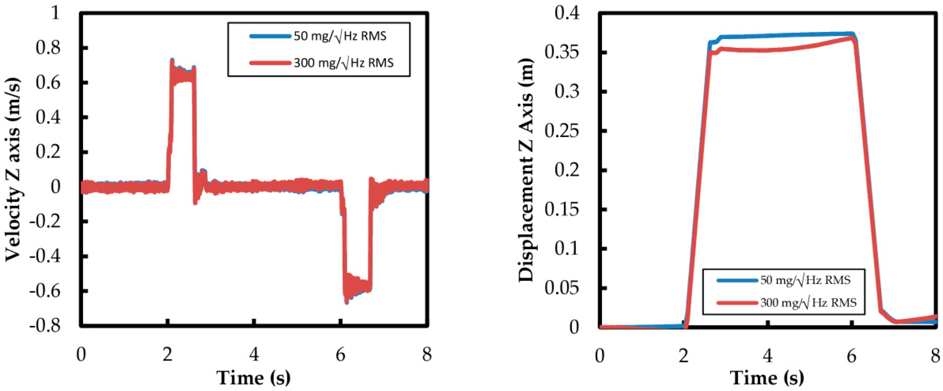
The results show two families of errors depending on the level of influence on the quality of results. First, the noise, the non-linearity and the cross-axis sensitivity show a negligible effect over the reconstruction of velocity and a very limited effect over the displacement. Only high levels of these errors are able to generate visible distortions in the reconstructed signals, creating a light twisting in the signals without a clear tendency of change.
On the other hand, the presence of any small level of bias in the acceleration signal produces a clear effect on the reconstruction of the velocity and intense influence on the displacement. The existence of bias produces a general slope and a light bending in the velocity and displacement, a quick shift of the results to unreal high levels. The quality indicators show that the drift in displacement is about an order of magnitude higher than velocity deviation; the error produces a larger effect during double integration of the acceleration in comparison with single integration, as has been already reported in the literature.
Finally, the saturation of the acceleration signal has been analyzed. Thus, the maximum signal of acceleration has been restricted to a certain value, where the full scale of the accelerometer is not enough for caption the real accelerations produced in the studied systems. This situation is expected to happen during the measurement of unknown operation conditions, where the level of acceleration to be measured is uncertain. In this case, there is a clear distortion in the velocity values which generates a clear displacement shift, mostly from the start of the movement of the system. The more characteristic effect observed in the velocity signal is the shift from the zero velocity level in the resting periods. This phenomena is evidently generated by the limited acceleration measurements during the velocity change phases of the hydraulic cylinder operating cycle. Mention that signal saturation produces limited distortion in velocity and displacement in comparison with the effect of the bias. It can be noted by lower EF [x,v] indicators.
In summary, the bias has been identified as the error more affecting reconstruction of the velocity and displacement in the Z axis of movement of the cylinder. At a lower level of influence, the signal saturation shows a notable effect during the data processing. Finally, the noise, the non-linearity and the cross-axis sensitivity have low level of influence in the results when restricted to expected values of error.
2.4. Y Axis Simulation Analysis
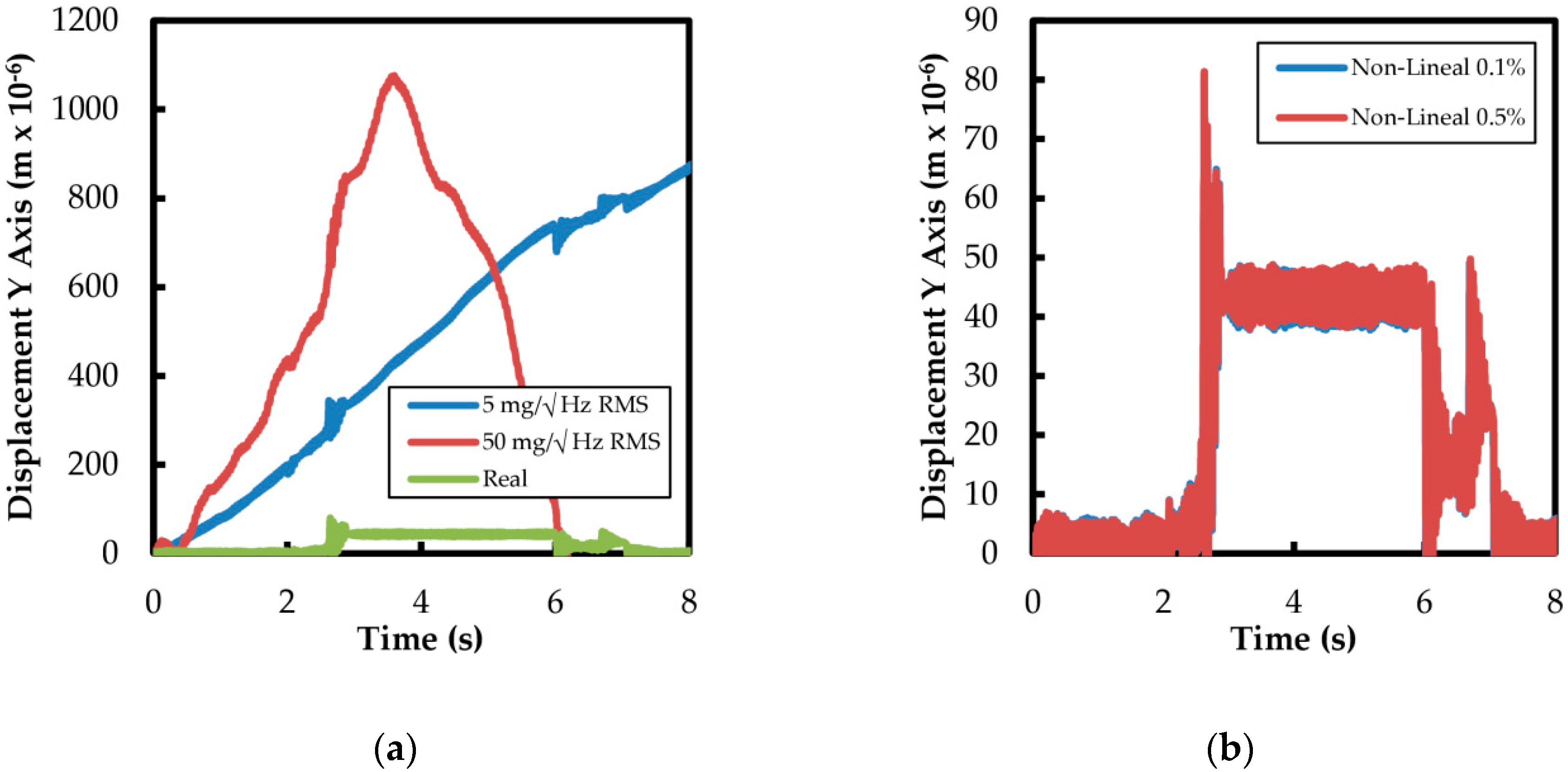
In comparison with the analysis of the Z axis, the Y axis simulation shows a clearly different behavior in relation with the influence of the errors, due to the different nature of the measured phenomena. First of all, the non-linearity has been identified as a negligible source of error, without relevant effect in the displacement measurement. On the other hand, the level of noise is a significant source of error in the reconstruction of the displacement; only very small levels of noise generate an extensive modification of the results, obtaining unreal values. The bias, as observed in the Z axis analysis, also generates an important slope in the curves. Both noise and bias errors produce a displacement curve several orders of magnitude away from the expected results, both in shape as in value. All these high deviations from real displacement of the calculated curves are summarized in the quality indicators for Y axis displacement showed in Table 3.
Finally, the cross-axis sensitivity, which had a negligible effect in Z axis, represents a significant source of error in the Y axis displacement reconstruction. In this case, even a very low amount of cross-axis sensitivity causes distortion in the results. So, the unreal resulting curve of Y axis displacement acquires the same shape of the Z axis but with some orders of magnitude less value. It’s clearly due to the low magnitude of the acceleration measured in Y axis in relation with the Z axis. Be noticed that the important deviations easily observed in the curves are not traduced in a very bad quality indicators. This singularity indicates the importance of the visual evaluation of the curves in order to validate the obtained results. In consequence, the quality indicators are mainly reliable in the comparison of different levels of similar error sources.
In summary, the results of the simulation of the reconstruction of the piston displacement in the Y axis show that this measurement is highly affected by the presence of errors. Thus, even simulating a hypothetical high quality acceleration sensor with extremely low level of errors (as showed with the blue line in Figure 13 and Figure 14), the experiment would result in false displacement values.
3. Experimental Results
The experimental assembly described in our previous work [8] has been updated by installing a triaxial accelerometer inside the piston. This sensor is able to monitor the accelerations generated by the extension and retraction movement (Z axis) and transversal displacements of the piston inside the cylinder body (X and Y axes), as described in Figure 15. Therefore, direct displacement and velocity readings (Measured) can be compared with the results obtained through the integration of the acceleration records (Calculated), as has been done in the simulation model. Integration of experimental data is performed by means of the trapezium rule; this method generates an estimated RSME [x] = 0.002 in the Z axis displacement calculation.
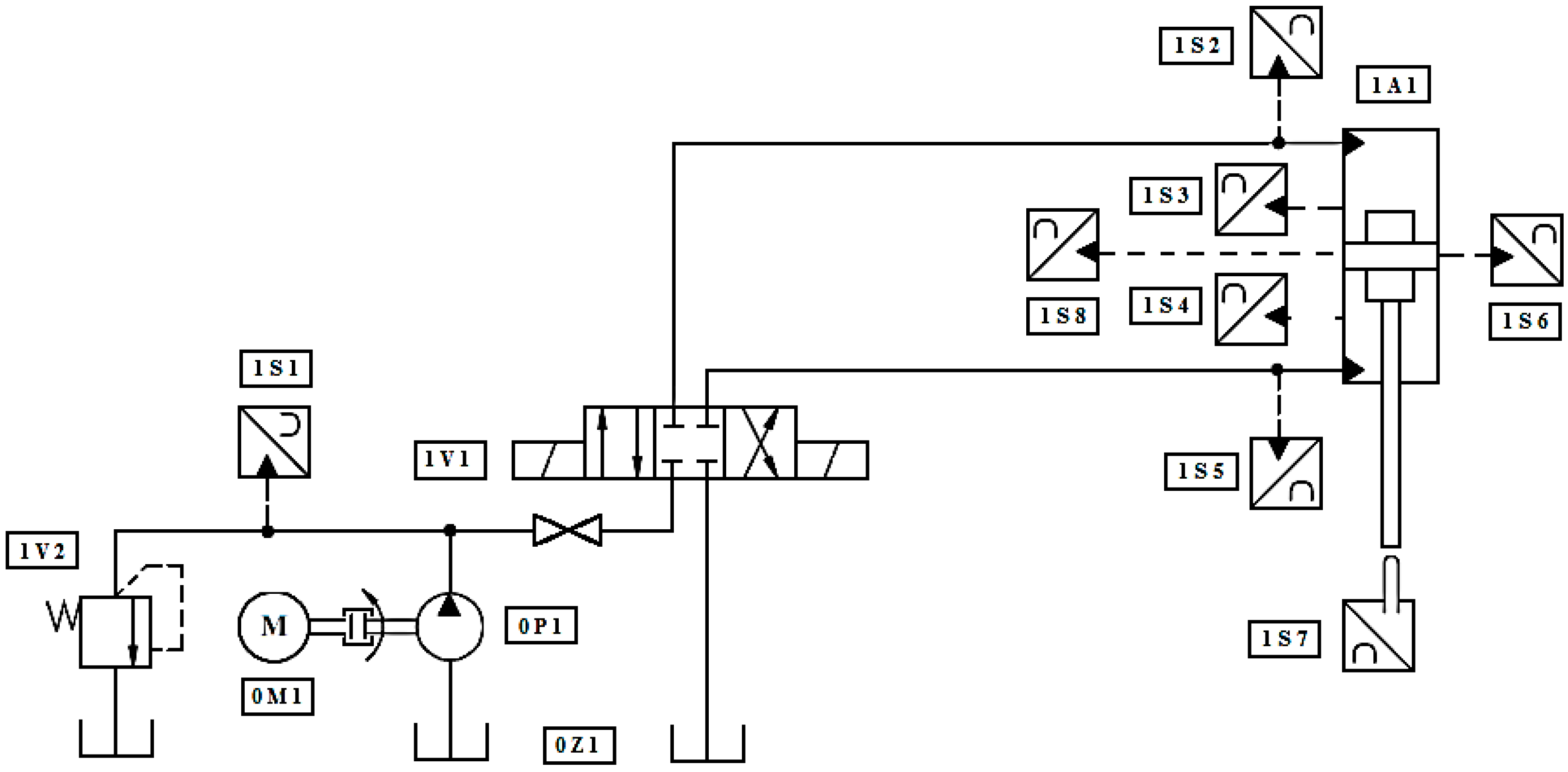
In summary, the experimental setup monitors a double effect hydraulic cylinder during its extension-retraction cycle. The Z axis, extension displacement of the cylinder, and Y axis displacements, axial piston displacement inside the cylinder barrel, are obtained by direct measure and indirect acceleration measure. The hydraulic circuit schema and the main components of the experimental set-up are described in Figure 16 and listed in Table 4. All the experiments have been performed with a hydraulic fluid temperature of 40 °C, inside the operating temperature range of the utilized sensors. The accelerometer used is a commercial model ADXL335 MEMS accelerometer by Analog Devices (Norwood, MA, USA), being its functional characteristics described in Table 1.
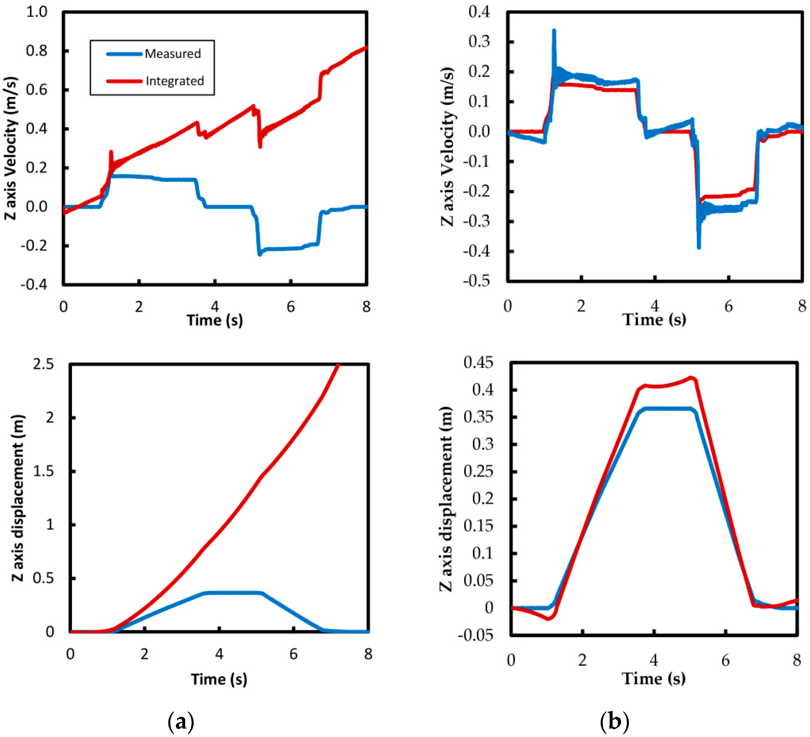
Figure 17 presents a comparison between the measured and calculated velocity and displacement, obtained during an experiment at 100 Bar pressure supply and a flow of 30 L/min. Right hand (a) is presented the raw data obtained, appearing a behavior mainly affected by bias error as already predicted by the model in Figure 10. The use of a simple correction method confirms the presence of this bias error; the subtraction of a 0.1% FS of bias in the acceleration data produces a big improvement in the results, as presented in Figure 17b. As can be noticed, the resulting corrected curves are already affected by other minor error sources, presumably a combination of non-linearity and cross-axis sensitivity. The corresponding quality indicators are showed in Table 5. It’s assumed that the noise is not a significant error source after any filtering of the acceleration records doesn’t improve after the double integration.
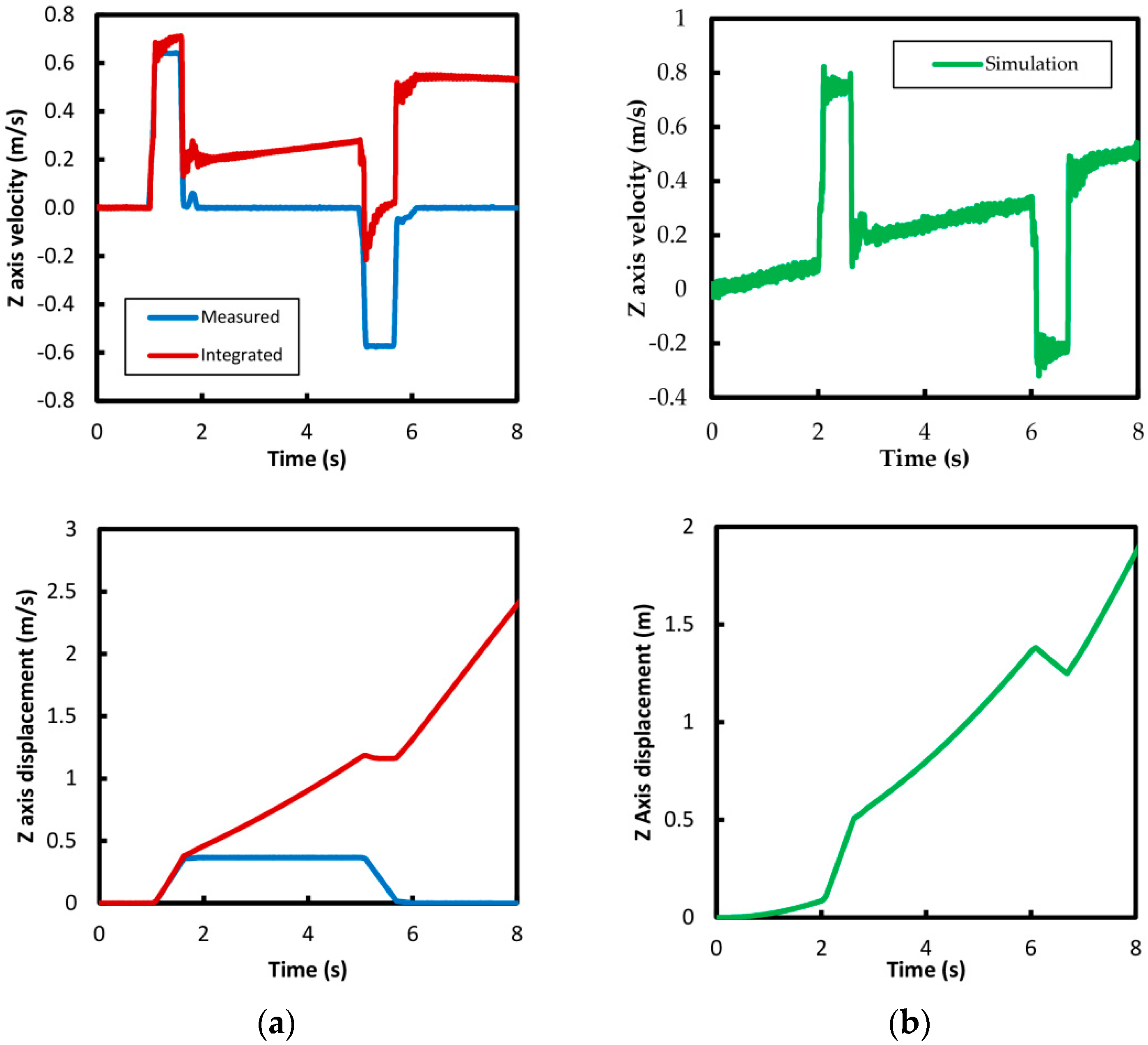
The same measurements are repeated for other experiment using 150 bar pressure supply and a maximum flow of 90 L/min. In this case, more severe functional conditions turn into a calculated behavior with big similarities with the observed for signal saturation, as exposed in Figure 11. More precisely, a certain degree of bias in the measured acceleration is also considered considering the previous results. As can be seen in the Figure 18, a modeled signal including 0.15% bias and signal saturation reveals similarities with the experimental results. Even so, there are several differences; first, the observed variable velocity slope, probably caused by the simplifications of the simulation mechanical model; second, the resulting acceleration response, that would minimize the effect of the saturation. Both modeled and experimental acceleration responses are depicted in Figure 19. Experimental records show concrete high power signals at high frequencies and good match with modeled medium and low frequencies records. Besides, possible crossed affectations between simultaneous measurement errors would be also a potential cause of the observed deviations, not considered in the presented study.
Evidently, the application of correction methods is not practical due to the saturation of the sensor and the resultant loss of information in the acceleration measurement. Hence, it’s recommended the selection of a suitable measurement sensor range or the restriction of the functional range of the measured system.
In case of Y axis measurement, the experimental results present a significant drift due to an important cross-axis sensitivity affectation. They are displayed in Figure 20 in comparison with Z axis records. In this case the displacement curve acquires the shape of the Z axis records but with several orders of magnitude less value. This undesirable behavior has already been predicted by the simulation results, as described in Figure 14b.
4. Conclusions
The development of a bond graph model for the simulation of a multi-axis low cost accelerometer has been successful in the forecast of the accuracy of velocity and displacement reconstruction from imperfect acceleration measurements, as has been corroborated from experimental results. Thus, the knowledge of the influence of the main error sources allows a suitable assessment of the measuring devices and eventual suppression methods during the signal manipulations.
More precisely, a significant difference in measurement reliability has been observed between the extension/retraction and transversal piston displacements inside the hydraulic cylinder body. The main cause is the distinct nature of the acceleration signals obtained of the two different movements. In consequence, the proposed simulation model of indirect displacement reconstruction can be useful in other interested engineering applications. It could be the case of similar electromechanical systems as displacement controllers of proportional valves spools. It would be an advantage during measuring strategy and sensor selection, results forecast and evaluation of data processing requirements.
The bias is the main distortion source detected in the calculation of the extension/retraction velocity and displacement, which has, fortunately, an easy suppression method. On the other hand, caution has to be taken in selection of the measurement range. A compromise is required between the best possible accuracy, associated with the tightest measuring range, and the avoidance of signal saturation during more extreme operating conditions measurement. Unpredictably, other error sources as noise and non-linearity, even considering an important level of error, have moderate effects in the observed performance of the studied system.
In contrast, the transversal displacements and velocities numerical results show important issues as a consequence of the acceleration measurement errors. Even simulating a hypothetical extremely high performance sensor the measurement of transversal displacements shows very high deviations to unreal values. Besides, the measurement strong affectation by several errors makes very difficult to get reliable results using correction algorithm.
Being the main objective of the acceleration measurement to obtain a simply procedure for measure the transversal displacements of the piston, the proposed model allows a reliable evaluation of different levels of accuracy in the acceleration measurement. From the results described above, the evaluated strategy for the required application isn’t suitable with the current low cost devices.
Author Contributions
The investigation was leaded and supervised by E.C. and J.F. Experimental works, data processing and illustrations were completed by A.A. and J.F. The manuscript was finalized by A.A., E.C. and J.F.
Funding
This research received no external funding.
Acknowledgments
We thank Pedro Roquet and Juan Jose Pérez from Roquet Group, S.A. who provided important hydraulic devices used in the research.
Conflicts of Interest
The authors declare no conflict of interest.
References
- Moschas, F.; Stiros, S. Measurement of the dynamic displacements and of the modal frequencies of a short-span pedestrian bridge using GPS and an accelerometer. Eng. Struct. 2011, 33, 10–17. [Google Scholar] [CrossRef]
- Thenozhi, S.; Yu, W.; Garrido, R. A novel numerical integrator for velocity and position estimation. Trans. Inst. Meas. Control 2013, 35, 824–833. [Google Scholar] [CrossRef]
- Stiros, S.C. Errors in velocities and displacements deduced from accelerographs: An approach based on the theory of error propagation. Soil Dyn. Earthq. Eng. 2008, 28, 415–420. [Google Scholar] [CrossRef]
- Wong, H.L.; Trifunac, M.D. Effects of cross-axis sensitivity and misalignment on the response of mechanical-optical accelerographs. Bull. Seism. Soc. Am. 1977, 67, 929–956. [Google Scholar]
- Thong, Y.K.; Woolfson, M.S.; Crowe, J.A.; Hayes-Gill, B.R.; Jones, D.A. Numerical double integration of acceleration measurements in noise. Meas. J. Int. Meas. Confed. 2004, 36, 73–92. [Google Scholar] [CrossRef]
- Edwards, T.S. Effects of aliasing on numerical integration. Mech. Syst. Signal Process. 2007, 21, 165–176. [Google Scholar] [CrossRef]
- Boore, D.M. Analog-to-digital conversion as a source of drifts in displacements derived from digital recordings of ground acceleration. Bull. Seismol. Soc. Am. 2003, 93, 2017–2024. [Google Scholar] [CrossRef]
- Algar, A.; Codina, E.; Freire, J. Experimental Study of 3D Movement in Cushioning of Hydraulic Cylinder. Energies 2017, 10, 746. [Google Scholar] [CrossRef]
- Boser, B.E.; Howe, R.T. Surface Micromachined Accelerometers. IEEE J. Solid-State Circuits 1996, 31, 366–375. [Google Scholar] [CrossRef]
- Grigorie, T.L. The Matlab/Simulink Modeling and Numerical Simulation of an Analogue Capacitive Micro-Accelerometer. Part 1: Open loop. In Proceedings of the MEMSTECH’2008, Polyana, Ukraine, 21–24 May 2008; pp. 105–114. [Google Scholar]
- Grigorie, T.L. The Matlab/Simulink Modeling and Numerical Simulation of an Analogue Capacitive Micro-Accelerometer. Part 2: Closed loop. In Proceedings of the MEMSTECH’2008, Polyana, Ukraine, 21–24 May 2008; pp. 115–121. [Google Scholar]
- Song, Z.; Sun, T.; Wu, J.; Che, L. System-level simulation and implementation for a high Q capacitive accelerometer with PD feedback compensation. Microsyst. Technol. 2015, 21, 2233–2240. [Google Scholar] [CrossRef]
- He, J.; Zhou, W.; Yu, H.; He, X.; Peng, P. Structural Designing of a MEMS Capacitive Accelerometer for Low Temperature Coefficient and High Linearity. Sensors 2018, 18, 643. [Google Scholar] [CrossRef] [PubMed]
- He, J.; Xie, J.; He, X.; Du, L.; Zhou, W. Sensors and Actuators A: Physical Analytical study and compensation for temperature drifts of a bulk silicon MEMS capacitive accelerometer. Sens. Actuators A Phys. 2016, 239, 174–184. [Google Scholar] [CrossRef]
- Caixin, W.; Jingxin, D.; Yunfeng, L.; Changde, Z. Nonlinearity of a Closed-Loop Micro-accelerometer. In Proceedings of the 16th IEEE International Conference on Control Applications Part of IEEE Multi-conference on Systems and Control, Singapore, 1–3 October 2007; pp. 1260–1265. [Google Scholar]
- Meng, Z.; Jing, H.; Tingting, Z.; Lichen, H.; Yacong, Z.; Wengao, L.; Zhongjian, C. Research on Nonlinearity of Closed-Loop Capacitive Accelerometer Resulting from Time- Division Force Feedback. In Proceedings of the 2012 IEEE International Conference on Electron Devices and Solid State Circuit (EDSSC), Bangkok, Thailand, 3–5 December 2012. [Google Scholar]
- Jingqing, H.; Meng, Z.; Tingting, Z.; Lichen, H.; Feng, W.; Yacong, Z.; Wengao, L.; Zhongjian, C. Linear Analysis of Closed Loop Capacitive Accelerometer Due to Distance Mismatch between Plates. In Proceedings of the 2012 IEEE International Conference on Electron Devices and Solid State Circuit (EDSSC), Bangkok, Thailand, 3–5 December 2012. [Google Scholar]
- Choi, J.; Lee, J.; Han, S.; Kim, S.; Hong, S.; Choi, J. A Readout Circuit with Novel Zero-g Offset Calibration for Tri-axes Capacitive MEMS Accelerometer. In Proceedings of the IEEE International Symposium on Circuits and Systems (ISCAS), Lisbon, Portugal, 24–27 May 2015; pp. 1062–1065. [Google Scholar]
- Wang, X.; Zhao, J.; Zhao, Y.; Xia, G.M.; Qiu, A.P.; Su, Y.; Xu, Y.P. A 0.4 µg Bias Instability and 1.2 µg/√Hz Noise Floor MEMS Silicon Oscillating Accelerometer with CMOS Readout Circuit. IEEE J. Solid-State Circuit 2017, 52, 472–482. [Google Scholar] [CrossRef]
- Yin, T.; Ye, Z.; Huang, G.; Wu, H.; Yang, H. A closed-loop interface for capacitive micro-accelerometers with pulse-width-modulation force feedback. Analog Integr. Circuits Signal Process. 2018, 94, 195–204. [Google Scholar] [CrossRef]
- Hong, Y.H.; Kim, H.K.; Lee, H.S. Reconstruction of dynamic displacement and velocity from measured accelerations using the variational statement of an inverse problem. J. Sound Vib. 2010, 329, 4980–5003. [Google Scholar] [CrossRef]
- Hong, Y.H.; Lee, S.G.; Lee, H.S. Design of the FEM-FIR filter for displacement reconstruction using accelerations and displacements measured at different sampling rates. Mech. Syst. Signal Process. 2013, 38, 460–481. [Google Scholar] [CrossRef]
- Zhu, W.H.; Lamarche, T. Velocity estimation by using position and acceleration sensors. IEEE Trans. Ind. Electron. 2007, 54, 2706–2715. [Google Scholar]
- Kim, J.; Kim, K.; Sohn, H. Autonomous dynamic displacement estimation from data fusion of acceleration and intermittent displacement measurements. Mech. Syst. Signal Process. 2014, 42, 194–205. [Google Scholar] [CrossRef]
- Arias-lara, D.; De-la-colina, J. Assessment of methodologies to estimate displacements from measured acceleration records. Measurement 2018, 114, 261–273. [Google Scholar] [CrossRef]
Figure 1.
Capacitive accelerometer operational schema.

Figure 2.
Block diagram of a proportional-integral-derivative (PID) closed loop control of an accelerometer (based on [12]). KF: Voltage-to-Force linear factor; KV: displacement-to-voltage amplification linear factor; LPF: Low Pass Filter.
Figure 2.
Block diagram of a proportional-integral-derivative (PID) closed loop control of an accelerometer (based on [12]). KF: Voltage-to-Force linear factor; KV: displacement-to-voltage amplification linear factor; LPF: Low Pass Filter.

Figure 3.
Bond graph model for Z axis displacement. modular flow source.

Figure 4.
Bond graph model for Y axis displacement.

Figure 5.
Displacement and velocity sources; (a) Z axis; (b) Y axis.

Figure 6.
Frequency response of the accelerometer model; (a) Bode diagram; (b) Step response.

Figure 7.
Ideal linearity, Bias and non-linearity sensor representation.

Figure 8.
Calculated velocity and displacement for Z axis; Noise error evaluation.

Figure 9.
Calculated velocity and displacement for Z axis; Non-linearity error evaluation.

Figure 10.
Calculated velocity and displacement for Z axis; Cross-axis sensitivity error evaluation.
Figure 10.
Calculated velocity and displacement for Z axis; Cross-axis sensitivity error evaluation.

Figure 11.
Calculated velocity and displacement for Z axis; Bias error evaluation.

Figure 12.
Calculated velocity and displacement for Z axis; Signal saturation error evaluation.

Figure 13.
Calculated displacement for Y axis; (a) noise and (b) non-linearity error evaluation.

Figure 14.
Calculated displacement for Y axis; (a) bias and (b) cross-axis sensitivity error evaluation.
Figure 14.
Calculated displacement for Y axis; (a) bias and (b) cross-axis sensitivity error evaluation.

Figure 15.
Hydraulic cylinder and accelerometer assembly schema.

Figure 16.
Hydraulic circuit and instrumentation schema.

Figure 17.
Experimental and calculated results of velocity and displacement in Z axis; (a) raw calculated results; (b) bias corrected calculated results.
Figure 17.
Experimental and calculated results of velocity and displacement in Z axis; (a) raw calculated results; (b) bias corrected calculated results.

Figure 18.
Experimental and calculated results of velocity and displacement in Z axis; (a) experimental results; (b) simulation results.
Figure 18.
Experimental and calculated results of velocity and displacement in Z axis; (a) experimental results; (b) simulation results.

Figure 19.
Z axis acceleration records and power spectrum; (a) simulation model; (b) experimental records.
Figure 19.
Z axis acceleration records and power spectrum; (a) simulation model; (b) experimental records.

Figure 20.
Calculated results of displacement in Y and Z axes; Cross-axis sensitivity affectation observed.
Figure 20.
Calculated results of displacement in Y and Z axes; Cross-axis sensitivity affectation observed.


Table 1.
Considered parameters of accelerometer model.
| Parameter | Value |
|---|---|
| Damping Coefficient 1 | 0.5 |
| Natural Frequency | 5500 Hz |
| Range | ±3 g |
| Bandwith | 550 Hz |
| Mass 1 | 2 μKg |
| Noise Density | 300 μg/√Hz RMS 2 |
| Cross-Axis Sensitivity | 1% |
| Nonlinearity | 0.3% |
1 Estimated value; 2 Root Mean Square.
Table 2.
Quality indicators in the Z axis signal calculations by error; velocity [v] and displacement [x].
Table 2.
Quality indicators in the Z axis signal calculations by error; velocity [v] and displacement [x].
| Error | CCC [v] (Adim) | RSME [v] (m2/s2) | FE [v] (%) | CCC [x] (Adim) | RSME [x] (m2) | FE [x] (%) |
|---|---|---|---|---|---|---|
| 50 mg/√Hz RMS | 1.00 | 0.01 | 1% | 1.00 | 0.01 | 2% |
| 300 mg/√Hz RMS | 1.00 | 0.01 | 1% | 1.00 | 0.01 | 7% |
| Bias 0.01% | 1.00 | 0.03 | 5% | 0.89 | 0.13 | 73% |
| Bias 0.1% | 0.93 | 0.16 | 36% | 0.23 | 0.54 | 331% |
| Bias 0.2% | 0.75 | 0.31 | 74% | −0.02 | 1.05 | 651% |
| Non-Lineal 0.5% | 1.00 | 0.01 | 1% | 1.00 | 0.01 | 4% |
| Non-Lineal 1% | 1.00 | 0.01 | 1% | 1.00 | 0.00 | 1% |
| Non-Lineal 2% | 1.00 | 0.01 | 0% | 1.00 | 0.02 | 6% |
| Cross-axis 1% | 1.00 | 0.01 | 0% | 1.00 | 0.01 | 2% |
| Cross-axis 2% | 1.00 | 0.02 | 2% | 1.00 | 0.01 | 1% |
| Saturation @3 g | 0.98 | 0.05 | 12% | 0.93 | 0.08 | 69% |
| Saturation @2.5 g | 0.94 | 0.11 | 26% | 0.50 | 0.27 | 194% |
Table 3.
Quality indicators in the signal reconstruction of displacement [x] in Y axis.
| Error | CCC [x] (Adim) | RSME [x] ×1000 (m2) | FE [x] (%) |
|---|---|---|---|
| 50 mg/√Hz RMS | 0.72 | 0.49 | 321% |
| 5 mg/√Hz RMS | 0.16 | 0.57 | 1147% |
| Bias 0.01% | −0.14 | 107.75 | 302,247% |
| Bias 0.001% | −0.14 | 10.81 | 30,348% |
| Non-Lineal 0.5% | 0.96 | 0.01 | 5% |
| Non-Lineal 0.1% | 0.95 | 0.01 | 2% |
| Cross-axis 1% | 0.89 | 2.40 | 4% |
| Cross-axis 0.01% | 0.90 | 0.24 | 5% |
Table 4.
Identification of the experimental set-up components.
| Description | Component |
|---|---|
| Variable flow piston pump | P1 |
| Electric motor | M1 |
| Reservoir | Z1 |
| Directional valve | V1 |
| Pressure relief valve | V2 |
| Hydraulic cylinder | A1 |
| Pressure Transmitter—Range 0 to 250 bar ± 1% FSO | S1 to S5 |
| Eddy-current Displacement transducer—Range 0 to 0.5 mm ± 0.02% FSO | S6 |
| Displacement transducer—Range 0 to 950 mm ± 0.02% FSO | S7 |
| Accelerometer—Range ±3 g ± 0.3% FSO | S8 |
Table 5.
Quality indicators in the Z axis signal calculations; Velocity [v] and displacement [x].
| Error | CCC [v] (Adim) | RSME [v] (m2/s2) | FE [v] (%) | CCC [x] (Adim) | RSME [x] (m2) | FE [x] (%) |
|---|---|---|---|---|---|---|
| Raw calculated | −0.22 | 0.29 | 493% | 0.30 | 0.07 | 1086% |
| Bias corrected | 0.99 | 9 × 10⁻⁴ | 7% | 0.99 | 6 × 10⁻⁴ | 6% |
© 2018 by the authors. Licensee MDPI, Basel, Switzerland. This article is an open access article distributed under the terms and conditions of the Creative Commons Attribution (CC BY) license (http://creativecommons.org/licenses/by/4.0/).
Share and Cite
MDPI and ACS Style
Algar, A.; Codina, E.; Freire, J. Bond Graph Simulation of Error Propagation in Position Estimation of a Hydraulic Cylinder Using Low Cost Accelerometers. Energies 2018, 11, 2603. https://doi.org/10.3390/en11102603
AMA Style
Algar A, Codina E, Freire J. Bond Graph Simulation of Error Propagation in Position Estimation of a Hydraulic Cylinder Using Low Cost Accelerometers. Energies. 2018; 11(10):2603. https://doi.org/10.3390/en11102603
Chicago/Turabian StyleAlgar, Antonio, Esteban Codina, and Javier Freire. 2018. "Bond Graph Simulation of Error Propagation in Position Estimation of a Hydraulic Cylinder Using Low Cost Accelerometers" Energies 11, no. 10: 2603. https://doi.org/10.3390/en11102603
Note that from the first issue of 2016, this journal uses article numbers instead of page numbers. See further details here.