A Novel Integrated Method to Diagnose Faults in Power Transformers

Abstract

In a smart grid, many transformers are equipped for both power transmission and conversion. Because a stable operation of transformers is essential to maintain grid security, studying the fault diagnosis method of transformers can improve both fault detection and fault prevention. In this paper, a data-driven method, which uses a combination of Principal Component Analysis (PCA), Particle Swarm Optimization (PSO), and Support Vector Machines (SVM) to enable a better fault diagnosis of transformers, is proposed and investigated. PCA is used to reduce the dimension of transformer fault state data, and an improved PSO algorithm is used to obtain the optimal parameters for the SVM model. SVM, which is optimized using PSO, is used for the transformer-fault diagnosis. The diagnostic-results of the actual transformers confirm that the new method is effective. We also verified the importance of data richness with respect to the accuracy of the transformer-fault diagnosis.

1. Introduction

Several advanced technologies can be used to monitor power-equipment, and the large amount of status data of used equipment helps make the power grid “smarter”. Power transformers are expensive and important components of the smart grid, and hub devices for power transformation and transmission [1,2,3,4]. Because various faults, such as discharge and overheating, can occur during the operation of transformers, many characteristics corresponding to the faults can be affected like dissolved gases (H₂, CH₄, C₂H₆, C₂H₄, C₂H₂, CO, etc.), organic compounds (methanol, ethanol and 2-furfural), as well as the current and power of the transformers [5]. The dissolved gas analysis (DGA) is a common tool for monitoring and identifying transformer’s faults. IEEE C57.104. and IEC 60599 provide different methods such as key gases, Doernenburg Ratio, Rogers, three basic gas ratio, Duval triangle, and so on. However, due to the complexity of the working environment and the process structure of the transformers, these methods are not enough to make a right judgement and cannot judge fault fuzzy boundary. According to [6], their accuracy rates are about in 60%, which means the ratio methods cannot account for the diagnostic criteria completely [7]. In addition, the concentrations of cellulose chemical markers in oil, such as methanol, ethanol and 2-furfural, are used as a determination mark for diagnosing transformer insulation failure, which still present many challenges for an accurate interpretation in real transformers [8].

To improve the accuracy of fault diagnosis, artificial intelligence and machine learning algorithm were added to the field of transformer-fault diagnosis (TFD), including fuzzy sets [9], artificial neural networks (ANN) [10], artificial immune networks [11], probabilistic neural networks [12], rough sets [13], and support vector machines (SVM) [14]. These algorithms provide ways to develop new TFD technologies. However, these algorithms have some disadvantages. For example, it is difficult to determine the selection of parameters of fuzzy sets, artificial immune networks and probabilistic neural networks, ANNs are easier to fall into local minimum, and the fault-tolerant ability and generalization ability of rough set are weak.

SVM is usually used as a classification tool. From early 2-category techniques, multi-class SVM have been developed and are more suitable for TFD. The accuracy of multi-class SVM is determined by the parameters of its kernel function and penalty factor. In order to improve the efficiency of SVM in processing large amounts of input fault data, principal component analysis (PCA) will be used. Moreover, to reduce the influence of human experience and subjective judgment on these parameters, a new Particle Swarm Optimization (PSO) is borrowed to search the optimized parameters. This way, the most suitable SVM parameters within the effective input data reflecting the transformer’s fault will be found. SVM integrated with PCA and PSO can improves the speed and accuracy of TFD considerably. This paper is organized as follows. Section 2 introduces the complete TFD procedure implemented by improved SVM; In Section 3, we compare the accuracy of transformer-fault diagnosis using different methods. We then verify the effectiveness of the proposed method, and analyze the effect of data richness on the accuracy of the fault diagnosis. Section 4 summarizes all results.

2. TFD Model Based on SVM Integrated with PCA and PSO

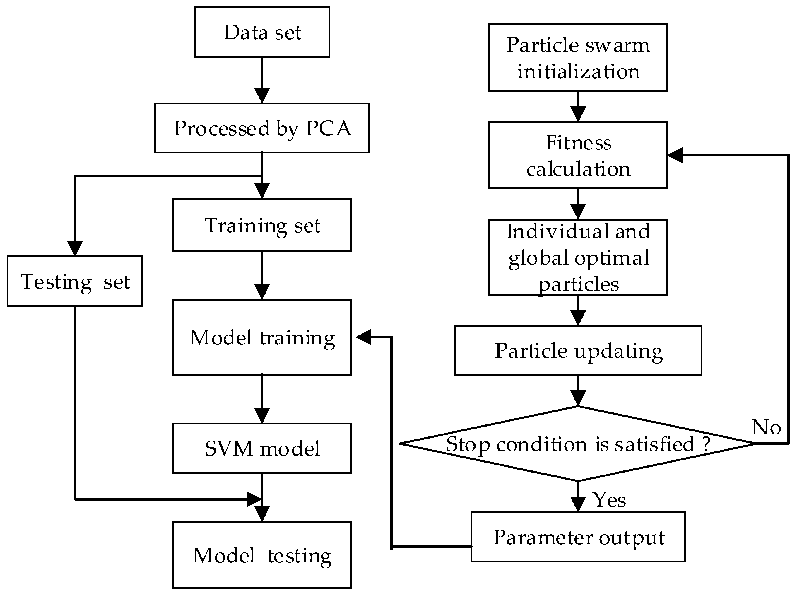
TFD model based on SVM integrated with PCA and PSO is shown in Figure 1. It includes two main parts. One is that a set of transformer fault data (Data set) such as the densities of the dissolved gases is preprocessed by PCA. The other is that the parameters of SVM model are searched and optimized by PSO.

2.1. Data Set Preprocessed by PCA

TFD is a complicated task. In order to improve the operating efficiency of the SVM when there are many transformer fault data, the data needs to be pre-processed before they are used to train the SVM model. PCA aims to reduce the dimensions of fault data and replaces them with fewer uncorrelated and unoverlapped data (called principal components). The number of principal components is selected by variance contribution rate indicating how much information is included.

Suppose the data set X has n groups and each group has p fault data and they construct an original data observation matrix:

$$X_{n\times p}=\left(\begin{array}{cccc}{x}_{11}& x_{12}& \cdots & x_{1p}\\ x_{21}& x_{22}& \cdots & x_{2p}\\ ⋮& ⋮& \ddots & ⋮\\ x_{n1}& x_{n2}& \cdots & x_{np}\end{array}\right)$$

(1)

To solve the principal components, it needs to find $i(i\le p)$ linear functions: $y_{ji}=A_i^T{X}_j$, where $j=1,\cdots ,n$, $X_j={(x_{j1},x_{j2},\cdots ,x_{jp})}^T$, and $A_i={(a_{1i},a_{2i},\cdots ,a_{pi})}^T$ is unknown. The amount of information of x is proportional to its variance. Letting $Y_{ji}={(y_{1i},y_{2i},\cdots ,y_{ni})}^T$ and to avoid $\mathrm{var}(Y_{ji})\to \infty$, ${\Vert A_i\Vert }^2=1$ Therefore, to obtain the maximum variance, the following equations of conditional extremes are formed:

$$\{\begin{array}{c}\max \mathrm{var}(Y_{ji})=\max A_i^T\sum A_i\\ A_i^T{A}_i=1\end{array}$$

(2)

where $\sum$ represents the covariance matrix.

Here Lagrange multiplier method is used to solve (2). The Lagrangian objective function is expressed as:

$$Q(A_i)=A_i^T\sum A_i-{\lambda }_j(A_i^T\sum A_i-1)$$

(3)

where the Lagrange multiplier ${\lambda }_j$ is the characteristic root of $\sum$ and $A_i$ is the corresponding eigenvector. Because $A_i\ne 0$ and $A_i^T\sum A_i=\mathrm{var}(A_i^T{X}_j)>0$, $\sum$ is positive definite and all characteristic roots are positive. Assuming that:

$${\lambda }_{`j}{}_1\ge {\lambda }_{`j}{}_2\ge \cdots \ge {\lambda }_{`jp}\ge 0$$

(4)

In the practical applications, only $p^{\prime }$ principal components will be selected, which satisfies ${\displaystyle \sum _{k=1}^{p^{\prime }}{\lambda }_{jk}}/{\displaystyle \sum _{i=1}^p{\lambda }_{ji}}\ge 0.85$. The k-th principal component for the j-th group is $y_{jk}=A_k^T{X}_j$. All the principal components form a vecor $Y_j={(y_{j1},y_{j2},\cdots ,y_{j{p}^{\prime }})}^T$.

2.2. Support Vector Machine

Suppose the j-th group of principal component $Y_j$ reflects the fault type $z_j$. We divide n groups of fault data into two sets. One set is the training set including l groups and the other set is the testing set including (n-l) groups. The training set is used to solve the parameters of SVM.

TFD is usually a multi-class problem to classify the categories in d ($d\ge 2$). The one-versus-one (OVO) method is adopted to extend 2-category SVM to multi-class SVM in this paper. This means it need to build SVM classifiers for any two different fault types $F_1$ and $F_2$ ($F_1,F_2\in \left\{z_j\right\}$), and there are a total of $d(d-1)/2$ classifiers. Assume a hyperplane function ${\omega }^T\phi (Y)+b=0$ can accurately separate $F_1$ and $F_2$ whose category labels are marked in −1 and 1. Here $\omega$ is the normal vector of the hyperplane, $b$ is the offset, and $\phi (\mathit{y})$ is nonlinear transformation function. For the optimal classification hyperplane, the following conditions should be satisfied:

$$\{\begin{array}{l}{\omega }^T\phi (Y_j)+b\ge 1,H_j=1\\ {\omega }^T\phi (Y_j)+b\le -1,H_j=-1\end{array}$$

(5)

and $H_j\in \left\{F_1,F_2\right\}$ is the classification of $Y_j$. In this case, $Y_j$ is mapped into a high-dimensional space.

The maximum margin between the plane and the nearest data is $1/\Vert \omega \Vert$. The greater it is, the better the classification confidence is. To increase the misclassification tolerance of SVM, a non-negative variable $e_j$ is introduced. Then the problem can be described as:

$$\{\begin{array}{l}\min \left(\frac{1}{2}{\Vert \omega \Vert }^2+C{\displaystyle \sum _{j=1}^l{e}_j}\right)\\ H_j\left({\omega }^T\phi \left(Y_j\right)+b\right)\ge 1-e_j\\ e_j\ge 0\end{array}$$

(6)

where $C$ is a constant named penalty factor and controls the punishment degree for misclassified data. Lagrange multiplier method is also used to solve (6). The corresponding Lagrangian function is:

$$L\left(\omega ,\sigma ,e_j,{\alpha }_j,{\beta }_j\right)=\frac{1}{2}{\Vert \omega \Vert }^2+C{\displaystyle \sum _{j=1}^l{e}_j}-{\displaystyle \sum _{j=1}^l{\alpha }_j\left[H_j\left({\omega }^T\phi \left(Y_j\right)+b\right)-1+e_j\right]}-{\displaystyle \sum _{j=1}^l{\beta }_j{e}_j}$$

(7)

where ${\alpha }_j>0$ and ${\beta }_j>0$ are the Lagrangian multipliers. After ${\alpha }_j(j=1,\cdots ,l)$, $\omega$ and b are solved, the final SVM classification function is:

$$f(Y_r^{\prime })=\mathrm{sgn}({\displaystyle \sum _{j=1}^l{\alpha }_j}{H}_{j}K(Y_r^{\prime },Y_j)+b)$$

(8)

where $Y_r^{\prime }$ ($r=l+1,\cdots ,n$) is the r-th group data in testing set, $K(Y_r^{\prime },Y_j)=\phi (Y_r^{\prime })\cdot \phi (Y_j)$ is the kernel function and we choose Gaussian radial basis function:

$$K(Y_r^{\prime },Y_j)=\exp \left(-\frac{{\Vert Y_r^{\prime }-Y_j\Vert }^2}{{\sigma }^2}\right)$$

(9)

where $\sigma$ is the parameter of kernel function.

2.3. Parameter Optimization in SVM Using Improved PSO

As mentioned before, when using SVM for fault diagnosis, we first need to determine the parameter $\sigma$ in kernel function (9) and penalty factor $C$ in (6). $\sigma$ affects the optimal classification performance and generalization ability of the SVM. $C$ is required to balance the learning machine’s complexity and empirical risk when determining the minimization of the objective function. Therefore, $\sigma$ and $C$ should be optimized. We use an improved PSO algorithm for optimization.

Assuming that in a 2-dimensional search space, there is a swarm including S particles, $q_s=\left(q_{s1},q_{s2}\right)(s=1,\cdots ,S)$. Each particle represents a potential solution and corresponds to a point in the 2-dimensional search space. Its velocity is $v_s={(v_{s1},v_{s2})}^T$ and optimal position is $P_s={\left(P_{s1},P_{s2}\right)}^T$. The optimal position within the S-particle population represents the global extremum, and it is set to $P_g={\left(P_{g1},P_{g2}\right)}^T$. The position-updating method for the particle’s velocity is expressed as:

$$v_{sd}\left(t+1\right)=wv\left(t\right)\cdot v_{sd}\left(t\right)+c_1\left(t\right)r_1\left(t\right)\left(P_{sd}\left(t\right)-q_{sd}\left(t\right)\right)+c_2\left(t\right)r_2\left(t\right)\left(P_{gd}\left(t\right)-q_{sd}\left(t\right)\right),d=1,2$$

(10)

$$q_{sd}\left(t+1\right)=q_{sd}\left(t\right)+v_{sd}\left(t+1\right)$$

(11)

where $c_1\left(t\right)$ and $c_2\left(t\right)$ are acceleration constants, $r_1(t)$ and $r_2(t)$ obey the (0,1)-uniform distribution, $w_{}v(t)$ is the speed update inertia weight representing the effect of the previous generation’s particles on the next generation particles’ velocity during the particle updating process.

Generally, the algorithm has relatively strong global optimization capability when $w_{}v(t)$ is large, and a relatively strong local optimization capability when $w_{}v(t)$ is small. However, the linear weight-adjustment method is single, and thus limits the optimization of the search ability. Aiming to change to single adjustment mode and better adapt to the complex environment, we present a new scheme for the stochastic inertia weight:

$$\{\begin{array}{l}wv(t)={\alpha }_1+\mathsf{\epsilon }/2.0,k\ge 0.05\\ wv(t)={\alpha }_2+\mathsf{\epsilon }/2.0,k<0.05\end{array}$$

(12)

$$k=\frac{\mathrm{fit}\left(t\right)-\mathrm{fit}\left(t\text{-}10\right)}{\mathrm{fit}\left(t\text{-}10\right)}$$

(13)

where $\mathrm{fit}\left(t\right)$ represents the optimal fitness value of the t-th generation and $\mathrm{fit}\left(t\text{-}10\right)$ is the optimal fitness value of the (t-10)-th generation, ${\alpha }_1$ and ${\alpha }_2$ are set to 0.5 and 0.4, respectively, reflecting the search ability in different situations, and $\mathsf{\epsilon }$ is a random value between 0 and 1. The acceleration constants $c_1\left(t\right)$ and $c_2$ are modified in:

$$\{\begin{array}{l}{c}_1(t)=c_1{}_1+(c_{12}-c_1{}_1)\frac{t}{T}\\ c_2(t)=c_{21}+(c_{22}-c_{21})\frac{t}{T}\end{array}$$

(14)

where $c_1(t)$ decreases linearly from the initial value $c_{11}$ to the final value $c_{12}$, while $c_2\mathrm{(}t\mathrm{)}$ increases linearly from $c_{21}$ to $c_{22}$.

3. Verification and Discussion

Based on the above mentioned SVM-diagnosis model, optimized using PSO, a code is made in MATLAB in which SVM algorithm is implemented directly by MATLAB toolkit [15]. Some real TFD examples are analyzed.

3.1. TFD Example 1

We analyze the dissolved-gas data for the existing 157 groups of transformers under normal and other fault conditions. The dissolved-gas data were detected from 6 types of real transformer faults: low-energy discharge fault (LE-D), high-energy discharge fault (HE-D), high temperature overheat fault (HT), medium temperature overheating fault (MT), medium and low temperature overheating failure (ML-T), and low temperature overheating fault (LT). 112 groups of data were selected as training samples, and the remaining 45 groups were used for testing. The distribution of the various faults and normal state samples are shown in

Table 1. Statistics of samples for training and testing, corresponding to various types of real faults.

Fault Type	Training Sample	Test Sample	Total
Normal	17	7	24
LE-D	23	10	33
HE-D	20	8	28
HT	23	10	33
MT	7	2	9
ML-T	13	5	18
LT	9	3	12
Total	112	45	157

.

In this analysis, the particle swarm number is 20, the maximum iteration number is 200, and the search intervals for parameters C and σ are [0.01, 1000] and [0.01, 1000], respectively. Furthermore, C = 15.8823 and σ = 50.1658.

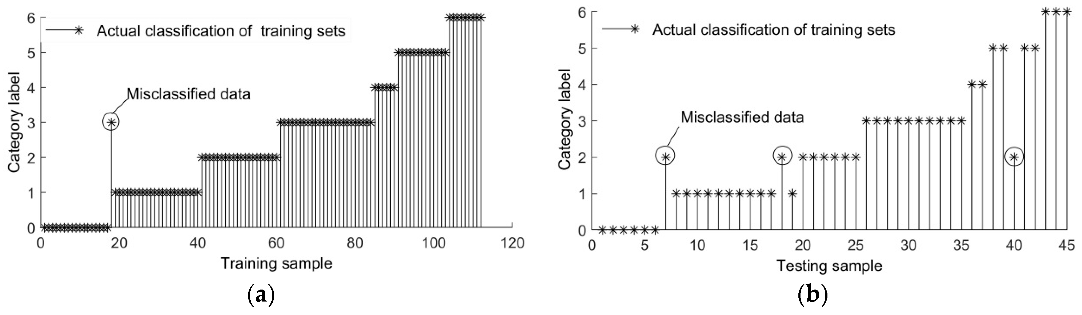
The fault diagnostic results of both the training set and the testing set are shown in Figure 2. Only one group of samples shows diagnosis errors among 112 groups of training samples (LE-D fault is diagnosed as HT fault), while 3 out of 45 samples yield diagnosis errors which are marked by circles. The accuracy reaches 93.33%. Diagnostic errors are either normal (diagnosed as HE-D), or LE-D fault (diagnosed as HE-D), or MT fault (diagnosed as HE-D). The results indicate that this method is relatively accurate and capable of realizing the aim of TFD.

We adopt the three-ratio method, Duval triangle method, back propagation neural network (BPNN), and SVM methods to diagnose the testing data set for comparison. The same set of data was used for all methods. During the test, BPNN selected a network structure with 13 hidden nodes.

Table 2. Accuracy rate for the different diagnostic methods of transformer.

Method	Three-Ratio	Duval Triangle	BPNN	SVM	This Paper
Accuracy rate	51.111%	42.222%	60.000%	75.556%	93.333%

shows the fault-diagnosis accuracy for different methods, when testing the same sample of transformer. The Duval triangle method shows the lowest accuracy. The three ratio method’s accuracy is better than The Duval triangle method, however, worse than other methods. Both of three-ratio and Duval triangle methods are obtained from typical accidents, and they will fail when dealing with some complicated faults. The accuracy of the neural-network algorithm (BPNN) is 60% and it will be improved if there are a lot of data. Compared with the BPNN and IEC methods, the SVM method shows a relatively good diagnosis. When the SVM parameters are optimized, the accuracy of the fault diagnosis improves substantially.

3.2. TFD Example 2

This section uses SVM optimized by PSO to analyze the fault and normal states from the 132 groups of data detected from real transformers. The data were from the oil-dissolved gas and SCADA. We also verified the impact of data richness on the results. The dissolved gases in the oil include C₂H₂, C₂H₄, C₂H₆, CH₄, CO, CO₂, H₂ and total hydrocarbon. The SCADA data include maximum current, minimum current, average current, maximum active power, minimum active power, average active power, maximum reactive power, minimum reactive power, and average reactive power. SVM optimized by PSO is used to diagnose the faults for three kinds of data: using only the dissolved gas data in oil, using only the SCADA data, and using all data. We used 112 groups as the training set and 20 groups as the testing set, and then judged the effect of data types on fault diagnosis.

In this experiment, the number for the particle swarm is 20, the maximum iteration number is 200, and the search interval of parameters $C$ and $\sigma$ are [0.01, 1000] and [0.01, 1000], respectively. The optimized parameter values and accuracy rate of different data types are shown in

Table 3. Fault-diagnostic results of transformer of different methods.

Types	Data	C	$\mathit{\sigma }$	Accuracy Rate
1	Dissolved gas data in oil only	5.023	0.709931	80%
2	SCADA data only	26.5631	7.3787	65%
3	Both above data	36.6918	0.074581	95%

.

For TFD results using only the dissolved gas in the oil, four out of 20 groups of normal data are misdiagnosed as fault state. However, the fault state is diagnosed correctly, and so the accuracy can reach 80% in general. The TFD results of using only SCADA data, as shown in Table 3, has many errors in the non-fault diagnosis. 13 out of 20 groups were correctly evaluated, and the accuracy is as high as 65%. For the TFD results using the dissolved gas in oil and the SCADA data as input data of SVM optimized by PSO, only 1 out of 20 groups of test data is erroneous (the non-fault condition is misdiagnosed as fault state). Hence, the accuracy of the fault diagnosis is 95%.

Comparing the diagnostic results for the above three data types, type 1 and type 2 can be used to diagnose most of the transformer states, but there errors are different, when diagnosing non-fault states. This is because each data type can reflect the fault states of the transformer to some extent, including part of the transformers’ state changes—but not completely. By combining these two kinds of data, more state information can be considered. The SVM optimized by PSO can learn the rich information from the data, thus improving the accuracy of the transformer-fault diagnosis.

4. Conclusions

A new fault-diagnosis technology for transformers, SVM optimized using PSO, was proposed in this paper, and it fully combines the advantages of the SVM and PSO. We used the dissolved-gas data in oil as the characteristic quantity and compared it with traditional methods as three-ratio, Duval triangle, and the artificial intelligence and machine learning algorithms as BPNN and SVM. The results showed that the proposed technology greatly improves the accuracy of the fault diagnosis. We also analyzed the effect of different data types of transformer on the TFD results. The data types included the dissolved-gas data in the transformer oil only, the SCADA data only, and both of them. The combination of the dissolved-gas data and SCADA data can improve the accuracy of the new technology substantially. This also testifies the importance of having sufficient data to perform an accurate transformer fault diagnosis.

The proposed method can be applied to prognostics and health management system in smart substations. It is noted that, if the amount of fault data is very big, it will take a long time to perform the fault diagnosis and it is inappropriate for on-line diagnosis; if the amount of fault data is not enough, its accuracy will be limited. The balance between the data amount and accuracy in its real applications needs further discussion.

References

- Zhao, Z.Y.; Tang, C.; Zhou, Q. Identification of Power Transformer Winding Mechanical Fault Types Based on Online IFRA by Support Vector Machine. Energies 2017, 10, 2022. [Google Scholar] [CrossRef]
- Kari, T.; Gao, W.S.; Zhao, D.B.; Zhang, Z.W.; Mo, W.X. An Integrated Method of ANFIS and Dempster-Shafer Theory for Fault Diagnosis of Power Transformer. IEEE Trans. Dielectr. Electr. 2018, 25, 360–371. [Google Scholar] [CrossRef]
- Wang, Y.Y.; Gong, S.L.; Grzybowski, S. Reliability evaluation method for oil-paper insulation in power transformers. Energies 2011, 4, 1362–1375. [Google Scholar] [CrossRef]
- Tenbohlen, S.; Coenen, S.; Djamali, M.; Müller, A.; Samimi, M.H.; Siegel, M. Diagnostic measurements for power transformers. Energies 2016, 9, 347. [Google Scholar] [CrossRef]
- Zheng, H.B.; Liao, R.J.; Grzybowski, S.; Yang, L.J. Fault diagnosis of power transformers using multi-class least square support vector machines classifiers with particle swarm optimization. IET Electr. Power Appl. 2011, 5, 691–696. [Google Scholar] [CrossRef]
- Zhao, A.X.; Zhang, C.T. DGA fault diagnosis based on the counter propagation neural network optimized by parallel genetic algorithm. In Proceedings of the 2013 IEEE International Conference of IEEE Region 10 (TENCON 2013), Xi’an, China, 22–25 October 2013; pp. 1–5. [Google Scholar]
- Ghoneim, S.S.M.; Taha, I.B.M.; Elkalashy, N.I. Integrated ANN-based proactive fault diagnostic scheme for power transformers using dissolved gas analysis. IEEE Trans. Dielectr. Electr. Insul. 2016, 23, 1838–1845. [Google Scholar] [CrossRef]
- Jalbert, J.; Lessard, M.C.; Ryadi, M. Cellulose chemical markers in transformer oil insulation part 1: Temperature correction factors. IEEE Trans. Dielectr. Electr. Insul. 2013, 2013. 20, 2287–2291. [Google Scholar] [CrossRef]
- Arispe, J.C.G.; Mombello, E.E. Power transformer diagnosis using FRA and Fuzzy Sets. IEEE Latin Am. Trans. 2015, 13, 2991–2997. [Google Scholar] [CrossRef]
- Seifeddine, S.; Khmais, B.; Abdelkader, C. Power transformer fault diagnosis based on dissolved gas analysis by artificial neural network. In Proceedings of the 2012 First International Conference on Renewable Energies and Vehicular Technology, Hammamet, Tunisia, 26–28 March 2012; pp. 230–236. [Google Scholar]
- Xiong, H.; Sun, C.X. Artificial immune network classification algorithm for fault diagnosis of power transformer. IEEE Trans. Power Deliv. 2006, 22, 930–935. [Google Scholar]
- Li, S.; Li, X.Y.; Wang, W.X. Fault Diagnosis of Transformer Based on Probabilistic Neural Network. In Proceedings of the Fourth International Conference on Intelligent Computation Technology and Automation, Shenzhen, China, 28–29 March 2011; Volume 1, pp. 128–131. [Google Scholar]
- Su, P.; Yuan, J.S.; An, X.L.; Li, Z.; Shen, T. Diagnosis method of transformer faults based on rough set theory. Electr. Power Sci. Eng. 2008, 24, 56–59. [Google Scholar]
- Bigdeli, M.; Vakilian, M.; Rahimpour, E. Transformer winding faults classification based on transfer function analysis by support vector machine. IET Electr. Power Appl. 2012, 6, 268–276. [Google Scholar] [CrossRef]
- Hsu, C.W.; Lin, C.J. A comparison of methods for multiclass support vector machines. IEEE Trans. Neural Netw. 2002, 13, 415–425. [Google Scholar] [PubMed] [Green Version]
Figure 1.
Transformer-fault diagnosis (TFD) model based on support vector machines (SVM) integrated with principal component analysis (PCA) and particle swarm optimization (PSO).
Figure 2.
Results of the transformer-failure diagnosis: (a) training sets; (b) testing sets.