Techno-Economic Analysis of Rural 4th Generation Biomass District Heating


1
Department of Design Engineering, Universidad de Seville, 41011 Seville, Spain
2
Department of Energy Engineering, University of Seville, 41092 Seville, Spain
3
Department of Electronic and Electromagnetism, University of Seville, 41012 Seville, Spain
*
Author to whom correspondence should be addressed.
Energies 2018, 11(12), 3287; https://doi.org/10.3390/en11123287
Submission received: 25 October 2018
/
Revised: 16 November 2018
/
Accepted: 21 November 2018
/
Published: 25 November 2018
(This article belongs to the Special Issue District Heating and Cooling Networks)
Abstract
:Biomass heating networks provide renewable heat using low carbon energy sources. They can be powerful tools for economy decarbonization. Heating networks can increase heating efficiency in districts and small size municipalities, using more efficient thermal generation technologies, with higher efficiencies and with more efficient emissions abatement technologies. This paper analyzes the application of a biomass fourth generation district heating, 4GDH (4th Generation Biomass District Heating), in a rural municipality. The heating network is designed to supply 77 residential buildings and eight public buildings, to replace the current individual diesel boilers and electrical heating systems. The development of the new fourth district heating generation implies the challenge of combining using low or very low temperatures in the distribution network pipes and delivery temperatures in existing facilities buildings. In this work biomass district heating designs based on third and fourth generation district heating network criteria are evaluated in terms of design conditions, operating ranges, effect of variable temperature operation, energy efficiency and investment and operating costs. The Internal Rate of Return of the different options ranges from 6.55% for a design based on the third generation network to 7.46% for a design based on the fourth generation network, with a 25 years investment horizon. The results and analyses of this work show the interest and challenges for the next low temperature DH generation for the rural area under analysis.
1. Introduction
Global warming is a major concern and urgent measures are required in a short time with the development of low carbon economy technologies [1]. At the same time, one of the key aspects to be developed by the scientific community in the coming years is an efficient energy distribution to cover the growth of the energy demand [2,3]. Building sector consumes 20% of the total energy in the world, with an expected increase ratio of 1.4% per year in the period between 2012 and 2040 [3]. By other side, of all new power generation plants installed worldwide in 2015, a 61% were based on renewable energies and an increase of this ratio is expected in the coming years [2].
District heating (DH) systems are considered as one of the most effective tools for an efficient and sustainable thermal energy distribution [4]. DH systems are centralized generation facilities, where thermal energy is distributed through a pipe network, which connects the thermal generation facility with the different consumption nodes at the buildings integrated in the system [5]. Thermal generation is centralized, and efficient and less contaminant heat generation equipment can be used, taking advantage of scaling up in the incorporation of combustion and emissions abatement technologies. It makes possible the efficient use of sustainable alternative energy sources. The energy efficiency of the global system is higher than the obtained with individual heating equipment [6] and, in addition, if renewable energy sources are used for thermal generation, a remarkable reduction in greenhouse gases emissions can be obtained [7].
European Directive 27/2012 [8] establishes a common framework to promote energy efficiency in Europe, in which DH networks have a relevant role. In previous research works methodologies to evaluate the potential of carrying out a massive implementation of different DH systems at a regional level have been developed [9,10]. Their results show how high impacts can be obtained if adequate methodologies for the selection, evaluation and implementation of district heating networks are used.
Distributed heating and cooling systems have a high potential for combining different renewable energy sources [10,11]. In heating systems, from the thermal point of view the most direct renewable energy sources to be integrated are biomass, solar energy [12,13,14] and geothermal energy [7,15]. Among them, the most direct integration is to use biomass as fuel, either renewable forestry products or sustainable agriculture biomass, with a higher potential in rural areas, where local biomass resource is available and the access to other primary energy sources is limited (i.e., natural gas).
The sustainability of biomass district heating rural networks will depend on the local biomass availability. The price of biomass depends on the proximity between the energy resource and the location of use [10,16,17]. The compensations that could arise in the local economy must be identified to ensure a stable and balanced development of heating networks in rural areas, the sector and the entire value chain [18]. Forestry activities can be a positive development in the economy of the area. Production of biomass for thermal generation can be a way to preserve rural areas, improve the quality of life of the municipality and to support the development of the territory that surrounds these activities. In this line, in reference [19], the impacts caused by the whole chain of biomass exploitation on the use of resources, human health and the environment are evaluated. The management of biomass, its transport, production of shavings, its treatments and its combustion are taken into account. It also analyzes the reduction of local pollution and GHG emissions that involves the displacement of a set of systems based on fossil fuels to a centralized production based on local biomass.
Among renewables, wind energy and photovoltaic can also be integrated for thermal integration of systems [7]. In reference [20] was shown how integration strategies between pipelines and buildings heat storage can be utilized to break the strong linkage of electric power and heat supply of CHP units, improving the operational flexibility of the system and reducing total operational costs.
DH networks are well established technologies, with an evolution along the year to incorporate advances in the operational strategies to increase their efficiency, to reduce distribution losses and to optimize their management [21]. The different generations of DH can be classified in terms of their operation temperatures, where operating temperatures have been lowered to reduce distribution heat losses [22,23].
There are different technologies that combined with DH systems improve efficiency and energy savings of the global system. Among the most interesting solutions is the combination of CHP biomass heating stations with DH systems. In reference [24] is shown how these installations are viable if the heating demand is high along the year, and it develops a methodology to evaluate the interest of these systems in order to improve the accuracy of the evaluation of the heating demand. It corrects the estimated demand for more accurate forecasting of heating demand that could lead to inadequate designs based on wrong performance parameters. The use of energy storage in these systems can reduce emission, operational cost and to enlarge the lifetime of existing CHP installations [25].
In reference [26] the different generations of DH are described. The third DH generation, and the most widely implemented nowadays, was developed in the period between 1980 and 2015. It is based on the distribution of liquid water at medium temperature, with temperatures below 100 °C. They use preinsulated and flexible pipes to facilitate their installation and to reduce installation and substitution costs. The fourth DH generation is currently under development. It is expected to have its maximum implementation in the period between 2020 and 2050. It is based on the distribution of water at a lower temperature, in the range between 30 °C and 60 °C. With this reduced operating temperatures, the thermal gradient between the heat transfer fluid and the environment is reduced and therefore the insulation requirements for controlling the thermal losses during distribution. Previous studies show the interest of low temperature district heating networks from the energy efficiency point of view [27]. The latest generation networks also make it easier to integrate these systems into Smart Energy Systems [23,28]. At the same time, the energy requirements of the buildings must be improved, improving their thermal behavior according to their location and energy demand characteristics. Internal equipment, as radiators, and end users habits, must be adapted for satisfying demand with these lower temperatures [29], increasing the available surface and adapting the heat demand profile.
Recent research activity in District Heating systems is oriented to integrate renewable energy sources with these systems and those that focus on the analysis or study of District Heating systems of low temperature, that is, investigate the applicability and viability of the heating urban low and very low temperature for buildings with high thermal performance. On this line different following European Commission funded projects: TEMPO [30], COOL DH [31], RELaTED [32], FLEXYNETS [33]. Among these European projects, the Project CELSIUS, develops Smart energy solutions. It deals with technical, social, economic and policy barriers for the development of new energy solutions. It shows the relevant role that DHC must have in the current and future sustainable Smart Cities [34,35].
In recent works the use of excess heat in industry as resource for district heating is analysed [36] with spatial and thermodynamic criteria. The analysis is expanded including the requirements linked to capital and operational expenditures.
This paper analyzes the application of a biomass fourth generation district heating, 4GDH, in a rural municipality. The heating network is designed to supply 77 residential buildings and eight public buildings, to replace the current individual diesel boilers and electrical heating systems. The development of the new fourth district heating generation, 4GDH, implies the challenge of combining using low or very low temperatures in the distribution network pipes and delivery temperatures in existing facilities buildings. A methodology is developed with the intention of comparing the operation of a biomass third generation or medium temperature network and a fourth generation or low temperature network. The aim is to compare operation modes estimated economic results. The evaluation methodology has common steps for both DH generations, so a common framework is established for a clear evaluation of results. The methodology is composed of two stages. The first stage carries out a technical analysis of the operation of the network with the objective of evaluating the total energy demand of the system, thermal load profile and pumping power consumption. The second stage performs an economic analysis of the operation of the network, based on the results obtained in the former stage, in order to determine the viability of the DH systems. The results show the viability of these DH and how it is affected by the operation with variable supply temperature.
2. Methodology
The objective of this methodology is to compare the viability and performance of two biomass District Heating networks (BioDHs), operating at two different levels one at medium temperature, with a design equivalent to the widely extended third generation DH design and other at low temperature equivalent to the fourth generation DH concept. The methodology has common stages for both cases but some steps differ according to the operation parameters of each one type of DH. The evaluation besides is extended to include the evaluation of the integration of another renewable source, wind energy, for providing electricity for pumping.
The proposed methodology comprises two different stages. In the first stage, the technical analysis of the operation of the network is performed. It drives to the sizing of the network and the definition of the energy profiles, thermal loads and pumping work. In the second stage, the economic analysis of the operation of the network is carried out, through a cost/benefit analysis. Stage one departs from the definition of the location of the system. Stage two departs from the results obtained in the previous stage and from the energy market characteristics, electricity and fuel costs definition.
2.1. Stage 1: Technical Analysis of DH Network Operation
Step 1: The first step defines the location of BioDH network, definition of the buildings to be supplied, and topographic conditions.
Step 2: After establishing the buildings to be supplied, the number of network users can be determined. On the other hand, it is also key to the determination of climatological data, mainly related to the minimum temperature, the degree days and the characterization of the wind resource throughout the year. The number of buildings included in the BioDH system will determine the total area to be heated, on which the heating demand depends proportionally, while the number of users will determine the SHW production requirements according to local regulations.
Step 3: Design of the network layout. Definition of its length, supply branches and integrated structure. It is defined as function of the supply zone characteristics: roads, altitude profiles, available area, other facilities, etc. The design minimizes network length, when possible, minimizing investment and civil works. The methodology of this stage is presented in Figure 1, while Figure 2 presents an example of the layout definition for the case study developed in Section 3.
With the heating demand, evaluated from the area to be heated, estimated from number of buildings and the demand of SHW, coming from the number of users, BioDH system heating power can be established, based on the minimum temperature and the thermal constant of the building, Kbuilding (1):
where P is the heat demanded (W), Ai is the surface (m2) of the outer wall (i), Kbuilding is the building’s thermal constant, Va inf is the infiltration air flow (m3/s), Ui is the global heat transfer coefficient (air/air) of this wall (W/ m2K), is the density of the outside air (kg/m3), Cp is the average specific heat of the outside air (Ws/kgK), Tc_indoor is the comfort indoor temperature (base temperature, 20 °C), and Tout is the outside temperature [9].
After determining the heating demand of the system, it is necessary to apply a simultaneity factor of the use of the network (2):
Simultaneity factor is a key parameter for an adequate sizing of any system with multiple users. The value of the simultaneity factor used in this work is based on an expression derived from the analysis of the surveys done with end users, although there are different methodologies to obtain it, and it can vary in function of the integrated systems [37].
In this step, the wind resource is also characterized, to evaluate the subsequent incorporation into the electric power for pumping. To do this, the equivalent wind hours of the wind turbine implantation area will be established, correcting the wind speed with the height.
Step 4: The theoretical thermal demand is established. Based on the climatological data of the location and the power of the network established in the previous section, the annual theoretical thermal demand that the network will have can be determined.
Up to this point, all the previous steps are common for the definition of a third generation medium temperature BioDH network and a fourth generation low temperature BioDH network. Up to this point, the energy requirements to be met by the BioDH system have been determined without taking into account the operating characteristic parameters of the network.
At this point, the operating parameters of each system are determined. These parameters are: supply temperature, return temperature, circulation flow and thermal drop in substations. The combination of these parameters will lead to different results in the technical analysis depending on the characteristics of the DH network. In this study, are compared BioDH networks of low and medium temperature where the fourth generation low temperature DH operates at temperatures below 60 °C and the third generation BioDH operates with temperatures in the range between 60 and 90 °C.
In this BioDH, the emissions in the biomass boilers are a main constraint to the design of the network and thermal power station. By other side, in the rural areas under analysis, most of the heating systems are based on individual biomass heaters and gasoil boilers. With the development BioDH the current heating systems are displaced by a more efficient heating systems that uses thermal generation technologies of higher efficiency and with more advanced and efficient emissions abatement technologies, as particles filters. It also includes the required maintenance operations in the boiler not always followed by small individual heating systems. The commercial biomass boilers proposed for this study case produce the following emission levels al 98% de rated power under EN (European Standard) 303-5:2013: 66 mg/Nm3 Dust, 62 mg/Nm3 of CO, 157 mg/Nm3 of NOx and 1 mg/Nm3 of Org. C.
Therefore the effective implementation of these BioDH systems will improve significantly the air quality and efficiency of the heating systems. However they have an important challenge in the social acceptance of biomass thermal stations within an urban location [10].
Another relevant aspect is the typology of the terminal heating devices already installed in houses. In the location under study, with a high level of energy poverty, of those users with heating by individual boilers, a 45% have modern low temperature radiators, 35% of houses have mid temperature old radiators, and 20% have radiating floor. For the implementation of low temperature DH, the substitution of these indoor terminal radiators prepared for high temperature implies an additional cost in comparison with higher temperature DH.
Step 5: In this step the size of the BioDH network is set. Based on the data obtained from the previous steps, the design of the layout gives the length of the network and pressure drops meanwhile the network power and the operating parameters provide mass flow and fluid velocity to meet energy requirements and sizing pipes. With the use of Equation (3), the flow rate can be obtained:
where Q is the flow rate (m3/s), Tflow is the flow temperature (K), Tret is the return temperature (K), Pdesign is the design power (W), c is the heat capacity of the fluid (J/(kg·K)) and ρ is the density (kg/m3).
As the operation parameters are specific for each type of BioDH system, the sizing of the network will also depend on the generation of DH that is being studied. Each mode of operation, therefore, will entail different pipe dimensions, an associated civil works, linked directly to required investments.
Step 6: After sizing the system, it is possible to evaluate the thermal losses along the distribution network. They depend directly on the diameter of the pipes and the average operating temperature of the system. The greater the diameter of the pipe, the lower the heat losses percentage produced per unit of flow; while at a lower average operating temperature, there is a lower thermal gradient between transport fluid and the external environment of the area, thus reducing thermal distribution losses significantly. To evaluate distribution thermal losses, pipes insulation is evaluated from the value of global heat transfer coefficient, Ui (W/(m2K)) provided in catalogue by pipe manufacturers.
To obtain the thermal distribution losses, Equations (4) and (5) can be applied:
where is the thermal gradient (K), Tflow is the flow temperature (K), Tret is the return temperature (K), Tground is the ground temperature (K), Tlosses is the thermal losses (W), u is the insulating capacity characteristic of the pipe W/(m*K)) and L is the length of the network (m).
Step 7: Finally, the total thermal demand and pumping power consumption are evaluated. To determine the total thermal demand, the theoretical thermal demand must be taken into account from heating and SHW demand, and corrected to compensate thermal losses. In this way, the total energy requirement from the generation thermal plant is established.
Once the total thermal demand and flows are known, the pumping costs can be determined, applying the electricity prices in each hourly section. If the use of wind power is evaluated to be used for supplying this pumping power, as included in this study integrating a microwind turbine, then this value is corrected with the quantification of the wind resource, data already obtained in Step 3, so that the net electric power consumption of the pumping group from the grid can be determined.
Both the total thermal demand and the pumping power consumption depend on the operation parameters of the network, therefore, these final results obtained in stage I, depend on the generation of BioDH that is under study.
For the low temperature DH, additional considerations must be taken into account, as the required maintenance and control for avoiding Legionella growth. It grows in humid environments with temperatures in the range el 20–50 °C, that correspond with the existing in low temperature DH. To control I, thermostatic valves in the primary network are required, and the maximum volume of water in heat exchangers is limited to three litres in order than the system operates below of 50 °C without using a recirculating external treatment [38]. Other possibility is to stress the network and tanks to periods of thermal shock to generate temporary adverse environments for Legionella growth. Besides, the use of decentralized substations can contribute with a higher control of temperature distribution along the network [39]. In reference [40] different models and solutions for low temperature DH are studied form the energy and economic points of view.
2.2. Economic Analysis of DH Network Operation
At this stage the economic analysis of the network operation is carried out, the scheme of the proposed methodology is shown in Figure 3. As data from previous stage are used, the final results will depend on the network characteristics allowing direct comparisons between different temperature designs and operation strategies. Likewise, there are data required for this step which are common for both types of networks, such as price of energy, the cost of the thermal plant and the indirect operating costs. As the purpose of this paper is to carry out a comparative study between the implantation of two different generation of DHs, the work will focus on what differs between both typologies of DH.
- -
- Capital Expenditure (CAPEX). The initial investment to carry out the implementation of the network depends on many factors, but the most relevant, for a defined location and thermal plant, is the diameter of the pipes, which affects to the required investment.
- -
- Operating Expenditure (OPEX). Operating costs depend on several parameters that vary directly with some operation parameters. The total thermal demand consists of: the theoretical thermal demand, which does not depend on the mode of operation, and the distribution heat losses that do vary with them. Thus, the thermal energy to be supplied by the station is function of the temperature of the DH network and therefore of the DH generation. This variation in total thermal demand will affect to fuel costs, biomass in this case, and pumping costs. So, the higher the requirement for thermal generation, the higher these costs will be. These costs will vary markedly throughout the year, due to the large variation in the demand of these types of heating networks. The indirect costs will not depend, in principle, on the fact that a specific BioDH generation design is being used, therefore, although it is an important aspect in the quantification of operating costs, it is not an aspect required for the comparison study.
- -
- Revenues from the BioDH System. The incomes generated by these systems come from the sale of thermal energy to users, therefore, the parameters to be taken into account in this section is the unit price of thermal energy sale and theoretical thermal demand. None of these aspects depends on the mode of operation of the BioDH system, therefore, the revenues structure generated by the two networks under the same coverage of demand will be the same. Therefore network profitability comparison involves the analysis of the operating costs and the investment.
- -
- Cost/Benefit Analysis. Once the investment, operating costs and generated incomes have been determined, the economic study of the network operation can be carried out, in order to analyze the cash flows that occur throughout the life cycle of the installation including taxes and other economic aspects. Different economic indexes can be used. In this work, for the comparison of DH networks is used the Internal Rate of Return. Investment return rate (IRR) is chosen as a parameter for evaluation and comparison of the projects (6) and it is defined as:where Iini is the initial investment, and LC is the life cycle of the system.
3. Results
In this section are presented the main results obtained of applying the methodology previously exposed, in order to design, size and evaluate the performance of two district networks under different technological design criteria that belong to different DH generations, so that afterwards, a comparative analysis between the results obtained for each one can be performed. In this way, it will be possible to discuss, in a real application case, the advantages and disadvantages of each type of technology proposed by the different generations of district heating. Simulations where implemented in MatLab (MathWorks, Natick, MA, USA).
The third generation BioDH works at medium temperature, with approximate supply and return temperatures of 85 °C and 60 °C respectively [41], in the case of facilities in Spain, with the consideration of the current typologies of radiators. The fourth generation BioDH works at a lower temperature level, with a network supply temperature of 55 °C and a return temperature at 25 °C [42].
For the case analysis proposed for implementation of the methodology, 85 buildings, belonging to Santiago de la Espada (Spain), will be integrated in the network, and the DH network will be composed of 173 stretches of pipes arranged in a branched way. Heating in buildings is provided with hot water radiators. In both cases is assumed that the life cycle of both DH facilities is the same, 25 years.
Table 1 shows the overall parameters and results of the BioDH system obtained from stage one. The power of the system is 1.9 MW. With a demand of 3.68 GWh per year, combining SHW and heating. The total length of the network is 1504 m to supply 85 buildings.
The cost of the electricty required for pumping varies along the day. The electricity tariff changes depending on the time slot: peak demand period, from 18:00 to 22:00 h, regular demand period, from 8:00 to 18:00 and from 22:00 to 24:00 h, and off-peak demand period from 0:00 to 8:00 h.
Figure 4a shows the flow of the medium and low temperature DH systems according to the demand of the BioDH system. Figure 4b relates the flows of the networks for the different months of the year.
In the low temperature network, the mass flow is smaller due to a higher temperature drop in the substations than the one in higher temperature networks. With a higher temperature drop a reduced mass flow is required to provide the same heating power.
Figure 4b shows that the difference between flows supplied by each type of network is more evident in the months with higher thermal demand. The results show that for the low temperature network the minimum and maximum flows throughout the year are 5.4 and 31.7 m3/h, respectively. However, in the case of the medium temperature network, the values of flow throughout the year are between the limits of 7.1 and 38.7 m3/h. In Figure 4 can be verified that the hottest periods correspond to the lower flow rates, that is, when the demand for heating is minimal or nonexistent and only SHW is required. This value is obtained for impulsion and return temperatures of the network fixed throughout the year. The mean average operating flow in the network throughout the year; for the case of the low temperature network it is 15.2 m3/h and for the medium temperature is 18.8 m3/h.
In this case a smart strategy control hasn’t been considered as operation temperatures cannot further reduced due to constrains associated with the installations of the buildings and to cover the comfort requirements for SHW and heating. These installation were developed for individual use and not considering their integration in DH networks.
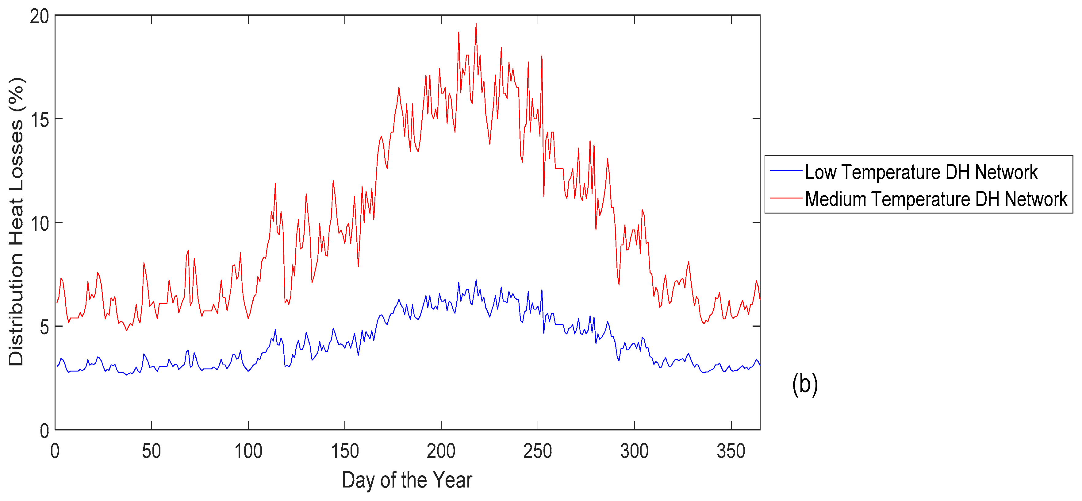
Figure 5a shows the influence of the demand on the thermal losses produced during the distribution of the heat transfer fluid.
The results show a difference between thermal losses in each type of network. Thermal losses along the year in the medium temperature network are approximately the double than those in the low temperature network. In this way, for the period of maximum demand, and lower external temperature, the thermal losses for the low and medium temperature networks are 2.63% and 4.74%, respectively; these are the minimum values. The maximum values, in percentage, appear when the demand is minimal, thermal losses values are 7.22% and 19.52% for a low and medium temperature network, respectively. This difference between the losses is due to the difference in operating temperatures of each network.
The losses that occur in the network depends on the thermal gradient that occurs between the operating temperatures of the network, the temperature of the ground around the pipe, insulation characteristics of the pipes and their size.
Ground temperature depends primarily on the ambient temperature and depth. From real experimental data of the temperature of the ground, measured at 20 cm of depth, an expression can be determined that relates the external ambient temperature to the temperature of the ground. These experimental data have been collected in an area close to the case study, within this project, it has not been validated for other geographical areas with different climatological and ground characteristics. In Figure 6 the relationship obtained from the experimental measurements is shown.
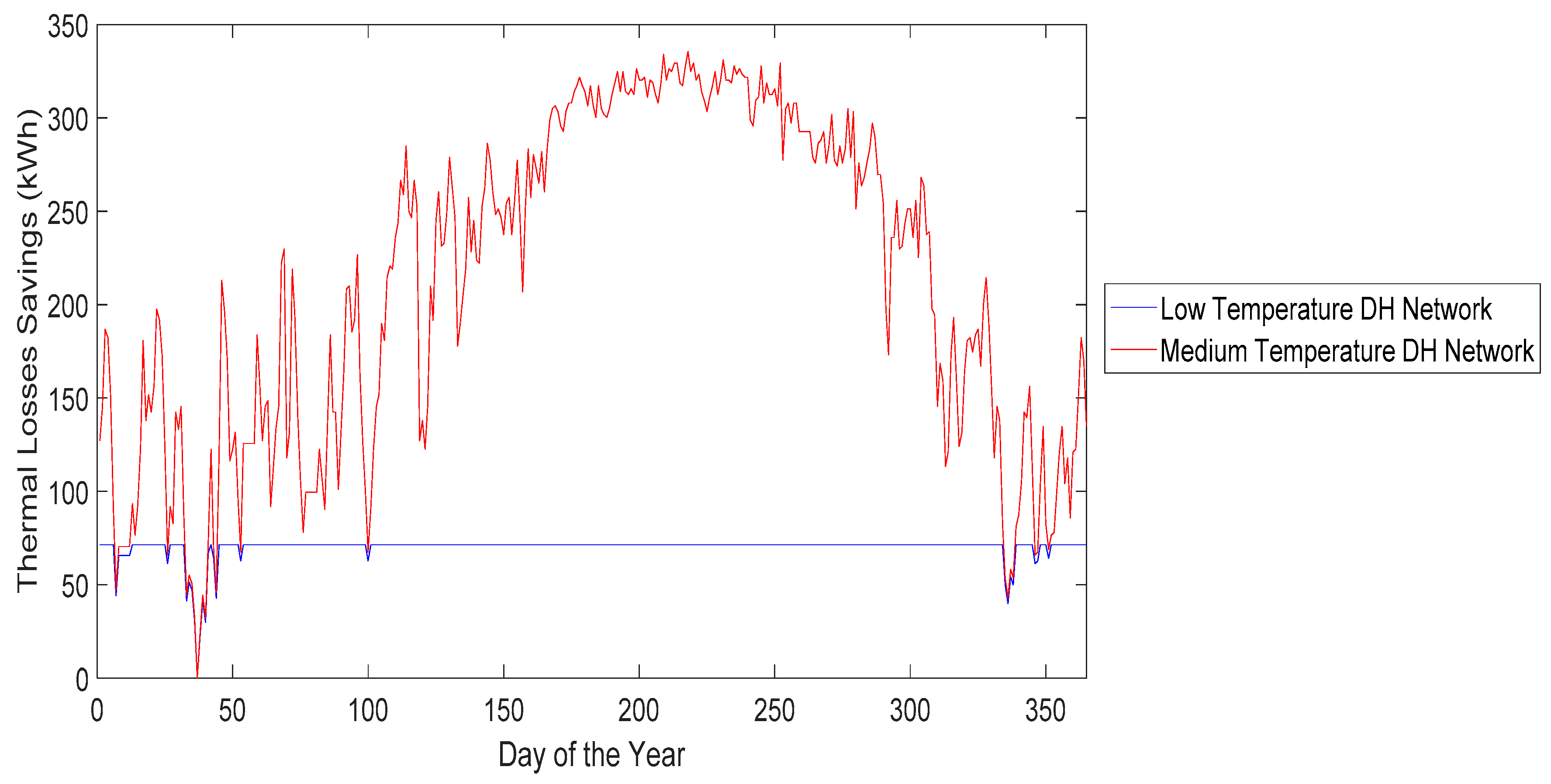
Another way to analyze thermal losses is by analyzing their total values with respect to the total demand. The variation of the thermal losses that occur in the low and medium temperature networks throughout the year are represented in Figure 7.
The evaluation of the investment associated to the different subsystems has been done according to [16,17], based on new construction systems. DH incomes will be the result of the energy sold by the sale price. For this case, end user sale price is set in 85 €/MWh. It implies to the end user 18% of savings compared with their current energy bills based on gasoil and wood in chimneys. This value has been set as function of the base line estimated as shown in [43]. Investment in DH is directly affected by pipes mean diameter. In the case of the low temperature network, due to a higher temperature drop in the thermal stations, mass flow circulating by pipes is lower and heating requirement can be maintained with smaller diameters. For the case under study it allows a reduction in pipes investment of 18.72%, and a reduced investment in the low temperature DH.
In Table 2 a comparison of the main results obtained in the design and calculation of the two district network designs is presented. The effect of installing a microwind turbine is also included to evaluate the effect on the total performance and system viability.
4. Discussion
To complete the study, parameters with a direct influence in the viability of the biomass DH system are analyzed. One parameter that can affect to the performance and viability of the district heating is to consider operation at constant network temperature or at variable temperature. The capacity of operating at variable temperature depends on the DH network technology. In the case of low temperature networks, which supply homes with radiators operating at low temperatures, the limit is to avoid using any auxiliary generation equipment. It constrains the supply and the minimum return temperature of the network, taking into account an indoor comfort temperature of 20 °C. On the other hand, for medium temperature networks, the limit is in the range of operation of the radiators, which in this case, operates with medium temperature. Then the limit can be obtained by analyzing the radiating surface and design temperatures of the radiators and comparing their capacity with the energy requirements that must be covered throughout the year. Therefore the variation range of operating temperatures is more limited for the case of low temperature DH networks.
If medium temperature the DH system operates with lower temperatures, Legionella growth risk increases, and control methodologies must be included in the medium temperature network in the same way that in the low temperature network.
By other side, the constraints associated with operating DH with variable temperature are not exclusively technological. Restrictions can be derived from legal aspects like the clauses in legal contracts related to energy supply, where it is usual to set a minimum supply temperature. For the development of variable operation DH this kind of clauses must be revised to guarantee the quality of heat supply and the optimal operation of the system. Besides end user awareness and formation about the most efficient use of indoor thermal facilities are required for a successful development. In [44] a thermos-hydraulic model for thermal networks is presented taking into account decentralized heating and cooling sources, variable temperature and mass flows and flow inversion.
The comparison of the losses that occur in a network with these designs, considering that the temperature of operation in the network is fixed or it can be variable is presented in Figure 8 and Figure 9. Figure 8 shows the results obtained at fixed and variable network temperatures for a low temperature network and Figure 9 shows the same analysis for a medium temperature network.
From these figures can be observed that in a medium temperature network, the supply and return temperatures can be lowered in a greater proportion than in a low temperature network, the losses that occur throughout the year in a medium temperature network can also be reduced in greater proportion. In the same way, the low temperature network is less sensitive to consider a variable network temperature.
Figure 10 analyzes losses reduction along the year. Energy savings, linked to losses reduction along the year, with a variable temperature operation in the low temperature network are 25.5 MWh meanwhile that in a medium temperature they are 38.6 MWh.
Another factor that affects to the network viability is the variation in the price of biomass. The price of biomass is a value that can vary quite significantly depending on the location where the DH network is located and constrains the viability of the project. Its effect is analyzed for the medium and low temperature networks for both operation strategies, with of fixed and variable supply temperatures.
Figure 11 shows the influence of the cost of biomass on the viability of the project. The best IRR values are provided by the low temperature network with variable working temperature; the worst values are provided by the medium temperature network with fixed values for supply and return temperatures.
In Figure 12 is presented the difference of IRR values between both networks as function of biomass price under the two different operation strategies, variable and fixed network temperature.
The energy savings that can be obtained in a medium temperature network, when considering variable working temperatures, is greater than in the case of a low temperature network. Therefore the IRR value will improve both for a medium temperature and low network, however, the IRR for medium temperature will be improved in a higher proportion reducing the differences between both designs.
In Figure 12 it is observed that on the one hand the IRR provided by a low temperature network is always greater than that which would be provided by a medium temperature network working under the same conditions, but that difference between IRR values is more noticeable when the fuel price is high and almost insignificant when the price is low. This is logical since in the low temperature network there are lower energy losses throughout the year, therefore, if the operating costs are high, this energy saving will be more relevant.
It can also be observed that the IRR difference, in the case that the networks work at variable impulsion and return temperatures, is lower. This is due to what has been said above that energy savings because of losses reduction that can be obtained in a medium temperature network, when considering variable working temperatures, is greater than in the case of a low temperature network. Then the difference between IRR values is smaller. Since low temperature networks have higher IRR values, these can be installed in areas where the price of biomass is high and where medium temperature networks would not provide viable IRR values.
5. Conclusions
In this work the differences between two generations of district heating applied to a specific case are analysed. The third generation of district heating networks uses higher supply and return temperatures, but with lower temperature drops compared to that produced in the fourth generation of district heating network systems. One of the most relevant characteristic of operation are thermal losses from the network to the terrain surrounding the pipes. With networks operating at lower temperatures, there is a reduced gradient, with the consequent reduction of thermal losses in the hot water distribution.
Regarding the total circulation flow, because the temperature drop in the substations is greater in the case of the fourth generation network, it is required that a lower flow rate circulates through them to supply the same thermal power. Since the flow rate through the network is lower, the diameters of the pipes can be reduced, thus causing a small increase in the pressure drop during operation.
This results in very similar pumping costs. This is due to the fact that in the fourth generation DH, lower flow rates are used in the operation of the system, but nevertheless, if smaller diameters are selected for reducing investment costs, pressure drops are greater.
These relationships between diameters, flows and heat losses are linked to the specific case study. Variations in network distribution and external conditions can lead to different ratios and a general rule of thumb cannot be derived.
Depending on the location characteristics, other renewable energy sources can be integrated. For the DH analyzed in this work the effect of integrating a microwind turbine is considered. As pumping cost are quite similar the savings obtained in both cases are similar.
The difference in the investment cost to carry out the projects is mainly due to the reduction in piping costs (materials and insulation) and civil works in the fourth generation DH network. This reduction is due to the fact that smaller dimensions of pipes and fittings are used, since it smaller circulation flow allows reduced diameters with controlled pressure drops. For the application case the investment savings are estimated in 44,220 €.
The reduction in operating costs that occurs in the district network of fourth generation is mainly due to the fact that the fuel required for the operation of the boiler is lower, since there are less thermal losses in the hot water distribution. When a fourth generation district network is implemented instead a third generation, as distribution thermal losses are reduced, there is a fuel saving of 4.8%.
Since the investment to be made and the operation costs of the fourth generation district network are lower, the payback period is lower, obtaining a more interesting investment profile as long as the income generated by both types is maintained. In this sense, the advantages of low temperature DH networks are clear when deciding from the investor’s point of view, in this case study. However, the development of heating networks in consolidated areas from the urban point of view involves the replacement of existing heating systems that currently operate at medium or high temperature. In these cases the application of the network at low temperature should consider the design of the interior installation of the houses and the adequateness of the network for maximum demand periods. The results of applying the methodology in a specific location and under operation conditions that allow to evaluate the differences in applying third and fourth DH network designs.
Analyzing the influence of operation with variable supply and return temperatures in low and medium temperature networks, it has been shown that energy losses are considerably reduced throughout the year. It has been shown, from the economic point of view, that it is always better when operating temperatures are variable, but it has also been seen that the variation suffered by the IRR of the project is not excessively high either. The price of biomass has been shown as key for viability of the project. The price of biomass can strongly vary different between projects with different locations, because this price depends strongly on the geographical area. When analyzing the profitability between the different types of networks, in the cases with a high cost of biomass, more interesting is to install a District Heating system with low temperature and with variable flow and return temperatures.
Author Contributions
Conceptualization, V.M.S.; Data curation, C.O.; Formal analysis, G.Q. Investigation, V.M.S. and G.Q.; Methodology, V.M.S.; Supervision, R.C.; Validation, C.O.; Writing—original draft, V.M.S. and R.C.
Funding
This research received no external funding.
Conflicts of Interest
The authors declare no conflict of interest.
Nomenclature
| z | Density (kg/m3) |
| Thermal gradient (K) | |
| Ai | Surface (m2) of the exterior wall (i) |
| c | Specific heat, J/(kg K) |
| Cp | Average specific heat of the exterior air (Ws/kgK) |
| CAPEX | Capital Expenditure |
| DH | District Heating |
| EN | European Standard |
| FS | Simultaneity factor |
| GDH | Generation of District Heating |
| Iini | Initial investment (€) |
| Kbuilding | Thermal constant of the building |
| L | Length of the network (m) |
| LC | Life cycle of the system (years) |
| OPEX | Operating Expenditure |
| P | Power demanded (kW) |
| Pdesign | Design power (kW) |
| Q | Flow rate (m3/s) |
| SHW | Sanitary Hot Water |
| Tc_indoor | Comfort temperature selected for the indoor space (base temperature, 20 °C) |
| Tflow | Flow temperature (K) |
| Tground | Ground temperature (K) |
| Tlosses | Thermal losses (W) |
| Tout | Temperature of the exterior air. |
| Tret | Return temperature (K) |
| u | Insulating capacity characteristic of the pipe W/(m*K)) |
| Ui | Global heat transfer coefficient (air/air) of this wall (W/ m2K) |
| Vainf | Flow of infiltration air (m3/s) |
References
- Lionello, P.; Scarascia, L. The relation between climate change in the Mediterranean region and global warming. Reg. Environ. Chang. 2018, 18, 1481–1493. [Google Scholar] [CrossRef]
- REthinking Energy 2017: Accelerating the global energy transformation. Available online: http://www.irena.org/publications/2017/Jan/REthinking-Energy-2017-Accelerating-the-global-energy-transformation (accessed on 25 October 2018).
- U.S. Energy Information Administration (EIA). 2018. Available online: https://www.eia.gov/ (accessed on 25 July 2018).
- Lake, A.; Rezaie, B.; Beyerlein, S. Review of district heating and cooling systems for a sustainable future. Renew. Sustain. Energy Rev. 2017, 67, 417–425. [Google Scholar] [CrossRef]
- Frederiksen, S.; Werner, S. District Heating and Cooling. Studentlitteratur; Studentlitteratur AB: Lund, Sweden, 2013. [Google Scholar]
- Sayegh, M.A.; Danielewicz, J.; Nannou, T.; Miniewicz, M.; Jadwiszcak, P.; Piekarska, K.; Jouhara, H. Trends of European research and development in district heating technologies. Renew. Sustain. Energy Rev. 2017, 68, 1183–1192. [Google Scholar] [CrossRef] [Green Version]
- Østergaard, P.A.; Mathiesen., B.V.; Möller, B.; Lund, H. A renewable energy scenario for Aalborg Municipality based on low-temperature geothermal heat, wind power and biomass. Energy 2010, 35, 4892–4901. [Google Scholar] [CrossRef]
- EUR-Lex-32012L0027-EN-EUR-Lex. Available online: https://eur-lex.europa.eu/eli/dir/2012/27/oj (accessed on 25 July 2018).
- Soltero, V.M.; Chacartegui, R.; Ortiz, C.; Velázquez, R. Evaluation of the potential of natural gas district heating cogeneration in Spain as a tool for decarbonisation of the economy. Energy 2016, 115, 1513–1532. [Google Scholar] [CrossRef]
- Soltero, V.M.; Rodríguez-Artacho, S.; Velázquez, R.; Chacartegui, R. Biomass universal district heating systems. E3S Web Conf. 2017, 22, 00163. [Google Scholar] [CrossRef] [Green Version]
- Østergaard, P.A.; Lund, H. A renewable energy system in Frederikshavn using low-temperature geothermal energy for district heating. Appl. Energy 2011, 88, 479–487. [Google Scholar] [CrossRef]
- Carpaneto, E.; Lazzeroni, P.; Repetto, M. Optimal integration of solar energy in a district heating network. Renew. Energy 2015, 75, 714–721. [Google Scholar] [CrossRef]
- Østergaard, P.A.; Andersen, A.N. Booster heat pumps and central heat pumps in district heating. Appl. Energy 2016, 184, 1374–1388. [Google Scholar] [CrossRef]
- Lizana, J.; Ortiz, C.; Soltero, V.M.; Chacartegui, R. District heating systems based on low-carbon energy technologies in Mediterranean areas. Energy 2017, 120, 397–416. [Google Scholar] [CrossRef]
- Aslan, A.; Yüksel, B.; Akyol, T. Effects of different operating conditions of Gonen geothermal district heating system on its annual performance. Energy Convers. Manag. 2014, 79, 554–567. [Google Scholar] [CrossRef]
- Soltero, V.; Chacartegui, R.; Ortiz, C.; Jesus, L.; Gonzalo, Q. Biomass District Heating Systems Based on Agriculture Residues. Appl. Sci. 2018, 8, 476. [Google Scholar] [CrossRef]
- Soltero, V.M.; Chacartegui, R.; Ortiz, C.; Velázquez, R. Potential of biomass district heating systems in rural areas. Energy 2018, 156, 132–143. [Google Scholar] [CrossRef]
- Fagarazzi, C.; Tirinnanzi, A.; Cozzi, M.; Di Napoli, F.; Romano, S. The Forest Energy Chain in Tuscany: Economic Feasibility and Environmental Effects of Two Types of Biomass District Heating Plant. Energies 2014, 7, 5899–5921. [Google Scholar] [CrossRef] [Green Version]
- Neri, E.; Cespi, D.; Setti, L.; Gombi, E.; Bernardi, E.; Vassura, I.; Passarini, F. Biomass Residues to Renewable Energy: A Life Cycle Perspective Applied at a Local Scale. Energies 2016, 9, 922. [Google Scholar] [CrossRef]
- Li, P.; Wang, H.; Lv, Q.; Li, W. Combined Heat and Power Dispatch Considering Heat Storage of Both Buildings and Pipelines in District Heating System for Wind Power Integration. Energies 2017, 10, 89. [Google Scholar] [CrossRef]
- Connolly, D.; Lund, H.; Mathiesen, B.V.; Werner, S.; Moller, B.; Persson, U.; Boermans, T.; Trier, D.; Qustergaard, P.A.; Nilesen, S. Heat Roadmap Europe: Combining district heating with heat savings to decarbonise the EU energy system. Energy Policy 2014, 65, 475–489. [Google Scholar] [CrossRef]
- Ziemele, J.; Gravelsins, A.; Blumberga, A.; Blumberga, D. Combining energy efficiency at source and at consumer to reach 4th generation district heating: Economic and system dynamics analysis. Energy 2017, 137, 595–606. [Google Scholar] [CrossRef]
- Ziemele, J.; Gravelsins, A.; Blumberga, A.; Blumberga, D. The Effect of Energy Efficiency Improvements on the Development of 4th Generation District Heating. Energy Procedia 2016, 95, 522–527. [Google Scholar] [CrossRef]
- Sartor, K.; Quoilin, S.; Dewallef, P. Simulation and optimization of a CHP biomass plant and district heating network. Appl. Energy 2014, 130, 474–483. [Google Scholar] [CrossRef] [Green Version]
- Sartor, K.; Dewallef, P. Optimized Integration of Heat Storage Into District Heating Networks Fed By a Biomass CHP Plant. Energy Procedia 2017, 135, 317–326. [Google Scholar] [CrossRef]
- Lund, H.; Werner, S.; Wiltshire, R.; Svendsen, S.; Thorsen, J.E.; Hvelpuld, F.; Mathiesen, B.V. 4th Generation District Heating (4GDH). Energy 2014, 68, 1–11. [Google Scholar] [CrossRef]
- Li, P.; Nord, N.; Ertesvåg, I.S.; Ge, Z.; Yang, Z.; Yang, Y. Integrated multiscale simulation of combined heat and power based district heating system. Energy Convers. Manag. 2015, 106, 337–354. [Google Scholar] [CrossRef]
- Li, H.; Wang, S.J. Challenges in Smart Low-temperature District Heating Development. Energy Procedia 2014, 61, 1472–1475. [Google Scholar] [CrossRef] [Green Version]
- Østergaard, D.S.; Svendsen, S. Replacing critical radiators to increase the potential to use low-temperature district heating-A case study of 4 Danish single-family houses from the 1930s. Energy 2016, 110, 75–84. [Google Scholar] [CrossRef]
- TEMPerature Optimisation for Low Temperature District Heating across Europe | Projects | H2020 | CORDIS | European Commission. Available online: https://cordis.europa.eu/project/rcn/212364_en.html (accessed on 25 July 2018).
- Cool Ways of Using Low Grade Heat Sources from Cooling and Surplus Heat for Heating of Energy Efficient Buildings with New Low Temperature District Heating (LTDH) Solutions. Available online: https://cordis.europa.eu/project/rcn/212356_en.html (accessed on 25 July 2018).
- REnewable Low TEmperature District. Available online: https://cordis.europa.eu/project/rcn/212357_en.html (accessed on 25 July 2018).
- Fifth Generation, Low Temperature, High EXergY District Heating and Cooling NETworkS. Available online: https://cordis.europa.eu/project/rcn/194622_en.html (accessed on 25 July 2018).
- Borelli, D.; Devia, F.; Lo Cascio, E.; Shenone, C.; Spolandore, A. Combined Production and Conversion of Energy in an Urban Integrated System. Energies 2016, 9, 817. [Google Scholar] [CrossRef]
- Perez, A.; Stadler, I.; Janocha, S.; Fermnando, C.; Bonvicini, G.; Tillmann, G. Heat recovery from sewage water using heat pumps in cologne: A case study. In Proceedings of the International Energy and Sustainability Conference, Koln, Germany, 30 Jun–1 July 2016; pp. 1–7. [Google Scholar]
- Bühler, F.; Petrović, S.; Holm, F.M.; Karlson, K.; Emegaard, B. Spatiotemporal and economic analysis of industrial excess heat as a resource for district heating. Energy 2018, 151, 715–728. [Google Scholar] [CrossRef]
- Winter, W.; Haslauer, T.; Obernberger, I. Simultaneity surveys in district heating networks: Results and project experience (Untersuchungen zur Gleich-zeitigkeit in Nahwärmenetzen: Ergebnisse und Projekterfahrungen). Euroheat Power 2001, 30, 42–47. (In German) [Google Scholar]
- Ianakiev, A.I.; Cui, J.M.; Garbett, S.; Filer, A. Innovative system for delivery of low temperature district heating. Int. J. Sustain. Energy Plan. Manag. 2017, 12, 1–28. [Google Scholar] [CrossRef]
- Yang, X.; Li, H.; Svendsen, S. Decentralized substations for low-temperature district heating with no Legionella risk, and low return temperatures. Energy 2016, 110, 65–74. [Google Scholar] [CrossRef]
- Yang, X.; Li, H.; Svendsen, S. Energy, economy and exergy evaluations of the solutions for supplying domestic hot water from low-temperature district heating in Denmark. Energy Convers. Manag. 2016, 122, 142–152. [Google Scholar] [CrossRef] [Green Version]
- Asociacion Técnica Española de Climatización y Refrigeracion (ATECYR). Guía Técnica de Instalaciones de Calefacción Individual; Institute for the Diversification and Saving of Energy: Madrid, Spain, 2010. [Google Scholar]
- Lund, R.; Østergaard, D.S.; Yang, X.; Mathiesen, B.V. Comparison of Low-temperature District Heating Concepts in a Long-Term Energy System Perspective. Int. J. Sustain. Energy. Plan. Manag. 2017, 12, 5–18. [Google Scholar] [CrossRef]
- Nielsen, S.; Grundahl, L.; Nielsen, S.; Grundahl, L. District Heating Expansion Potential with Low-Temperature and End-Use Heat Savings. Energies 2018, 11, 277. [Google Scholar] [CrossRef]
- Van der Heijde, B.; Fuchs, M.; Ribas Tugores, C.; Schweiger, G.; Sartor, K.; Basciotti, D.; Muller, D.; Nutsch-Geusen, C.; Wetter, M.; Helsen, L. Dynamic equation-based thermo-hydraulic pipe model for district heating and cooling systems. Energy Convers. Manag. 2017, 151, 158–169. [Google Scholar] [CrossRef]
Figure 1.
Stage I methodology.

Figure 2.
Network layout. Main distribution network (red lines) and secondary distribution network (yellow and orange lines).
Figure 2.
Network layout. Main distribution network (red lines) and secondary distribution network (yellow and orange lines).

Figure 3.
Stage II methodology.

Figure 4.
(a) Flow rate of medium and low temperature DH networks as function of thermal demand. (b) Flow rate for mean and low temperature DH networks along the year.
Figure 4.
(a) Flow rate of medium and low temperature DH networks as function of thermal demand. (b) Flow rate for mean and low temperature DH networks along the year.


Figure 5.
(a) Percentage of distribution heat losses for medium and low temperature DH networks as function of thermal demand, (b) Percentage of distribution thermal losses in the medium and low temperature DH networks along the year.
Figure 5.
(a) Percentage of distribution heat losses for medium and low temperature DH networks as function of thermal demand, (b) Percentage of distribution thermal losses in the medium and low temperature DH networks along the year.


Figure 6.
Relationship between ambient temperature and terrain temperature measured at 20 cm depth.

Figure 7.
(a) Distribution heat losses for medium and low temperature DH networks as function of thermal demand, (b) Distribution thermal losses in the medium and low temperature DH networks along the year.
Figure 7.
(a) Distribution heat losses for medium and low temperature DH networks as function of thermal demand, (b) Distribution thermal losses in the medium and low temperature DH networks along the year.

Figure 8.
Comparison of losses in a low temperature network along the year with fixed and variable network temperatures.
Figure 8.
Comparison of losses in a low temperature network along the year with fixed and variable network temperatures.

Figure 9.
Comparison of losses in a medium temperature network along the year with fixed and variable network temperatures.
Figure 9.
Comparison of losses in a medium temperature network along the year with fixed and variable network temperatures.

Figure 10.
Energy savings in low and medium temperature networks operating at variable network temperatures.
Figure 10.
Energy savings in low and medium temperature networks operating at variable network temperatures.

Figure 11.
Influence of the cost of biomass on DH viability with different operation strategies.

Figure 12.
Influence of the cost of biomass on IRR difference between a network of low and medium temperature, with fixed and variable operating temperatures of the network.
Figure 12.
Influence of the cost of biomass on IRR difference between a network of low and medium temperature, with fixed and variable operating temperatures of the network.


Table 1.
Common characteristics of both DH networks.
| Parameter | Value |
|---|---|
| Thermal power generated (kW) | 1909 |
| Heating demand (MWh) | 3434 |
| SHW Demand (MWh) | 248.4 |
| Number of buildings | 85 |
| Surface of the buildings (m2) | 9078 |
| Network length (m) | 1504 |
| Minimum temperature of the area (99) (°C) | −9.3 |
| Setpoint temperature in buildings (°C) | 20 |
| Average temperature of the ground (°C) | 8.9 |
| Thermal constant of the building (kW/°C) | 88.38 |
| Equivalent wind hours | 2462 |
| Electricity cost, period 1, peak hours (€/kWh) | 0.138 |
| Electricity cost, period 2, regular hours(€/kWh) | 0.104 |
| Electricity cost, period 3, off-peak hours(€/kWh) | 0.069 |
| Biomass Cost (€/MWh) | 30.00 |
Table 2.
Main operating parameters for both DH networks.
| Main operating Parameters | Third Generation Network. Medium Temperature | Fourth Generation Network. Low Temperature |
|---|---|---|
| Supply Temperature | 85 °C | 55 °C |
| Return temperature | 60 °C | 25 °C |
| Flow rate at design conditions | 44.00 m3/h | 36.10 m3/h |
| Average distribution pipes diameter | 101.27 mm | 89.72 mm |
| Pressure drop at rated conditions | 7.141 bar | 8.699 bar |
| Total Heat Demand | 4038 MWh | 3845 MWh |
| Annual thermal losses | 355.6 MWh | 161.9 MWh |
| Rated operation thermal losses (%) | 9.66% | 4.40% |
| Annual pumping costs | 14,964 € | 14,246 € |
| Annual wind turbine savings | 2198 € | 2093 € |
| Wind turbine savings (%) | 12.20% | 12.81% |
| Annual biomass cost | 121,145 € | 115,335 € |
| Equivalent performance hours | 2115 | 2014 |
| Total inversion | 1,080,898 € | 1,036,678 € |
| Annual total operational costs | 136,741 € | 130,200 € |
| Payback25 years | 15.34 years | 13.16 years |
| IRR25 years | 6.55% | 7.46% |
© 2018 by the authors. Licensee MDPI, Basel, Switzerland. This article is an open access article distributed under the terms and conditions of the Creative Commons Attribution (CC BY) license (http://creativecommons.org/licenses/by/4.0/).
Share and Cite
MDPI and ACS Style
Soltero, V.M.; Chacartegui, R.; Ortiz, C.; Quirosa, G. Techno-Economic Analysis of Rural 4th Generation Biomass District Heating. Energies 2018, 11, 3287. https://doi.org/10.3390/en11123287
AMA Style
Soltero VM, Chacartegui R, Ortiz C, Quirosa G. Techno-Economic Analysis of Rural 4th Generation Biomass District Heating. Energies. 2018; 11(12):3287. https://doi.org/10.3390/en11123287
Chicago/Turabian StyleSoltero, Víctor M., Ricardo Chacartegui, Carlos Ortiz, and Gonzalo Quirosa. 2018. "Techno-Economic Analysis of Rural 4th Generation Biomass District Heating" Energies 11, no. 12: 3287. https://doi.org/10.3390/en11123287
Note that from the first issue of 2016, this journal uses article numbers instead of page numbers. See further details here.