Hybrid Short-Term Load Forecasting Scheme Using Random Forest and Multilayer Perceptron †


1
School of Electrical Engineering, Korea University, 145 Anam-ro, Seongbuk-gu, Seoul 02841, Korea
2
Software Policy & Research Institute (SPRi), 22, Daewangpangyo-ro 712 beon-gil, Bundang-gu, Seongnam-si, Gyeonggi-do 13488, Korea
*
Author to whom correspondence should be addressed.
†
This paper is an extended version of our paper published in Proceedings of the 2018 IEEE International Conference on Big Data and Smart Computing (BigComp), Shanghai, China, 15–18 January 2018.
Energies 2018, 11(12), 3283; https://doi.org/10.3390/en11123283
Submission received: 31 October 2018
/
Revised: 19 November 2018
/
Accepted: 21 November 2018
/
Published: 25 November 2018
(This article belongs to the Special Issue Short-Term Load Forecasting by Artificial Intelligent Technologies)
Abstract
:A stable power supply is very important in the management of power infrastructure. One of the critical tasks in accomplishing this is to predict power consumption accurately, which usually requires considering diverse factors, including environmental, social, and spatial-temporal factors. Depending on the prediction scope, building type can also be an important factor since the same types of buildings show similar power consumption patterns. A university campus usually consists of several building types, including a laboratory, administrative office, lecture room, and dormitory. Depending on the temporal and external conditions, they tend to show a wide variation in the electrical load pattern. This paper proposes a hybrid short-term load forecast model for an educational building complex by using random forest and multilayer perceptron. To construct this model, we collect electrical load data of six years from a university campus and split them into training, validation, and test sets. For the training set, we classify the data using a decision tree with input parameters including date, day of the week, holiday, and academic year. In addition, we consider various configurations for random forest and multilayer perceptron and evaluate their prediction performance using the validation set to determine the optimal configuration. Then, we construct a hybrid short-term load forecast model by combining the two models and predict the daily electrical load for the test set. Through various experiments, we show that our hybrid forecast model performs better than other popular single forecast models.
1. Introduction
Recently, the smart grid has been gaining much attention as a feasible solution to the current global energy shortage problem [1]. Since it has many benefits, including those related to reliability, economics, efficiency, environment, and safety, diverse issues and challenges to implementing such a smart grid have been extensively surveyed and proposed [2]. A smart grid [1,2] is the next-generation power grid that merges information and communication technology (ICT) with the existing electrical grid to advance electrical power efficiency to the fullest by exchanging information between energy suppliers and consumers in real-time [3]. This enables the energy supplier to perform efficient energy management for renewable generation sources (solar radiation, wind, etc.) by accurately forecasting power consumption [4]. Therefore, for a more efficient operation, the smart grid requires precise electrical load forecasting in both the short-term and medium-term [5,6]. Short-term load forecasting (STLF) aims to prepare for losses caused by energy failure and overloading by maintaining an active power consumption reserve margin [5]. It includes daily electrical load, highest or peak electrical load, and very short-term load forecasting (VSTLF). Generally, STLF is used to regulate the energy system from 1 h to one week [7]. Accordingly, daily load forecasting is used in the energy planning for the next one day to one week [8,9].
A higher-education building complex, such as a university campus, is composed of a building cluster with a high electrical load, and hence, has been a large electric power distribution consumer in Korea [10,11,12]. In terms of operational cost management, forecasting can help in determining where, if any, savings can be made, as well as uncovering system inefficiencies [13]. In terms of scheduling, forecasting can be helpful for improving the operational efficiency, especially in an energy storage system (ESS) or renewable energy.
Forecasting the electrical load of a university campus is difficult due to its irregular power consumption patterns. Such patterns are determined by diverse factors, such as the academic schedule, social events, and natural condition. Even on the same campus, the electrical load patterns among buildings differ, depending on the usage or purpose. For instance, typical engineering and science buildings show a high power consumption, while dormitory buildings show a low power consumption. Thus, to accurately forecast the electrical load of university campus, we also need to consider the building type and power usage patterns.
By considering power consumption patterns and various external factors together, many machine learning algorithms have shown a reasonable performance in short-term load forecasting [3,4,6,8,14,15,16,17]. However, even machine learning algorithms with a higher performance have difficulty in making accurate predictions at all times, because each algorithm adopts a different weighting method [18]. Thus, we can see that there will always be randomness or inherent uncertainty in every prediction [19]. For instance, most university buildings in Korea show various electrical load patterns which differ, depending on the academic calendar. Furthermore, Korea celebrates several holidays, such as Buddha’s birthdays and Korean Thanksgiving days, called Chuseok, during the semester, which are counted on the lunar calendar. Since the campus usually remains closed on the holidays, the power consumption of the campus becomes very low. In such cases, it is difficult for a single excellent algorithm to make accurate predictions for all patterns. However, other algorithms can make accurate predictions in areas where the previous algorithm has been unable to do so. For this purpose, a good approach is to apply two or more algorithms to construct a hybrid probabilistic forecasting model [14]. Many recent studies have addressed a hybrid approach for STLF. Abdoos et al. [20] proposed a hybrid intelligent method for the short-term load forecasting of Iran’s power system using wavelet transform (WT), Gram-Schmidt (GS), and support vector machine (SVM). Dong et al. [21] proposed a hybrid data-driven model to predict the daily total load based on an ensemble artificial neural network. In a similar way, Lee and Hong [22] proposed a hybrid model for forecasting the monthly power load several months ahead based on a dynamic and fuzzy time series model. Recently, probabilistic forecasting has arisen as an active topic and it could provide quantitative uncertainty information, which can be useful to manage its randomness in the power system operation [23]. Xiao et al. [18] proposed no negative constraint theory (NNCT) and artificial intelligence-based combination models to predict future wind speed series of the Chengde region. Jurado et al. [24] proposed hybrid methodologies for electrical load forecasting in buildings with different profiles based on entropy-based feature selection with AI methodologies. Feng et al. [25] developed an ensemble model to produce both deterministic and probabilistic wind forecasts that consists of multiple single machine learning algorithms in the first layer and blending algorithms in the second layer. In our previous study [12], we built a daily electrical load forecast model based on random forest. In this study, to improve the forecasting performance of that model, we first classify the electrical load data by pattern similarity using a decision tree. Then, we construct a hybrid model based on random forest and multilayer perceptron by considering similar time series patterns.
The rest of this paper is organized as follows. In Section 2, we introduce several previous studies on the machine learning-based short-term load forecasting model. In Section 3, we present all the steps for constructing our hybrid electrical load forecasting model in detail. In Section 4, we describe several metrics for performance a comparison of load forecasting models. In Section 5, we describe how to evaluate the performance of our model via several experiments and show some of the results. Lastly, in Section 6, we briefly discuss the conclusion.
2. Related Work
So far, many researchers have attempted to construct STLF using various machine learning algorithms. Vrablecová et al. [7] developed the suitability of an online support vector regression (SVR) method to short-term power load forecasting and presented a comparison of 10 state-of-the-art forecasting methods in terms of accuracy for the public Irish Commission for Energy Regulation (CER) dataset. Tso and Yau [26] conducted weekly power consumption prediction for households in Hong Kong based on an artificial neural network (ANN), multiple regression (MR), and a decision tree (DT). They built the input variables of their prediction model by surveying the approximate power consumption for diverse electronic products, such as air conditioning, lighting, and dishwashing. Jain et al. [27] proposed a building electrical load forecasting model based on SVR. Electrical load data were collected from multi-family residential buildings located at the Columbia University campus in New York City. Grolinger et al. [28] proposed two electrical load forecasting models based on ANN and SVR to consider both events and external factors and performed electrical load forecasting by day, hour, and 15-min intervals for a large entertainment building. Amber et al. [29] proposed two forecasting models, genetic programming (GP) and MR, to forecast the daily power consumption of an administration building in London. Rodrigues et al. [30] performed forecasting methods of daily and hourly electrical load by using ANN. They used a database with consumption records, logged in 93 real households in Lisbon, Portugal. Efendi et al. [31] proposed a new approach for determining the linguistic out-sample forecasting by using the index numbers of the linguistics approach. They used the daily load data from the National Electricity Board of Malaysia as an empirical study.
Recently, a hybrid prediction scheme using multiple machine learning algorithms has shown a better performance than the conventional prediction scheme using a single machine learning algorithm [14]. The hybrid model aims to provide the best possible prediction performance by automatically managing the strengths and weaknesses of each base model. Xiao et al. [18] proposed two combination models, the no negative constraint theory (NNCT) and the artificial intelligence algorithm, and showed that they can always achieve a desirable forecasting performance compared to the existing traditional combination models. Jurado et al. [24] proposed a hybrid methodology that combines feature selection based on entropies with soft computing and machine learning approaches (i.e., fuzzy inductive reasoning, random forest, and neural networks) for three buildings in Barcelona. Abdoos et al. [20] proposed a new hybrid intelligent method for short-term load forecasting. They decomposed the electrical load signal into two levels using wavelet transform and then created the training input matrices using the decomposed signals and temperature data. After that, they selected the dominant features using the Gram–Schmidt method to reduce the dimensions of the input matrix. They used SVM as the classifier core for learning patterns of the training matrix. Dong et al. [21] proposed a novel hybrid data-driven “PEK” model for predicting the daily total load of the city of Shuyang, China. They constructed the model by using various function approximates, including partial mutual information (PMI)-based input variable selection, ensemble artificial neural network (ENN)-based output estimation, and K-nearest neighbor (KNN) regression-based output error estimation. Lee and Hong [22] proposed a hybrid model for forecasting the electrical load several months ahead based on a dynamic (i.e., air temperature dependency of power load) and a fuzzy time series approach. They tested their hybrid model using actual load data obtained from the Seoul metropolitan area, and compared its prediction performance with those of the other two dynamic models.
Previous studies on hybrid forecasting models comprise parameter selection and optimization technique-based combined approaches. This approach has the disadvantages that it is dependent on a designer’s expertise and exhibits low versatility [18]. On the other hand, this paper proposes data post-processing technique combined approaches to construct a hybrid forecasting model by combining random forest and multilayer perceptron (MLP).
3. Hybrid Short-Term Load Forecasting
In this section, we describe our hybrid electrical load forecasting model. The overall steps for constructing the forecasting model are shown in Figure 1. First, we collect daily power consumption data, time series information, and weather information, which will be used as independent variables for our hybrid STLF model. After some preprocessing, we build a hybrid prediction model based on random forest and MLP. Lastly, we perform a seven-step-ahead (one week or 145 h ahead) time series cross-validation for the electrical load data.
3.1. Dataset
To build an effective STLF model for buildings or building clusters, it is crucial to collect their real power consumption data that show the power usage of the buildings in the real world. For this purpose, we considered three clusters of buildings with varied purposes and collected their daily power consumption data from a university in Korea. The first cluster is composed of 32 buildings with academic purposes, such as the main building, amenities, department buildings, central library, etc. The second cluster is composed of 20 buildings, with science and engineering purposes. Compared to other clusters, this cluster showed a much higher electrical load, mainly due to the diverse experimental equipment and devices used in the laboratories. The third cluster comprised 16 dormitory buildings, whose power consumption was based on the residence pattern. In addition, we gathered other data, including the academic schedule, weather, and event calendar. The university employs the i-Smart system to monitor the electrical load in real time. This is an energy portal service operated by the Korea Electric Power Corporation (KEPCO) to give consumers electricity-related data such as electricity usage and expected bill to make them use electricity efficiently. Through this i-Smart system, we collected the daily power consumption of six years, from 2012 to 2017. For weather information, we utilized the regional synoptic meteorological data provided by the Korea Meteorological Office (KMA). KMA’s mid-term forecast provides information including the date, weather, temperature (maximum and minimum), and its reliability for more than seven days.
To build our hybrid STLF model, we considered nine variables; month, day of the month, day of the week, holiday, academic year, temperature, week-ahead load, year-ahead load, and LSTM Networks. In particular, the day of the week is a categorized variable and we present the seven days using integers 1 to 7 according to the ISO-8601 standard [32]. Accordingly, 1 indicates Monday and 7 indicates Sunday. Holiday, which includes Saturdays, Sundays, national holidays, and school anniversary [33], indicates whether the campus is closed or not. A detailed description of the input variables can be found in [12].
3.2. Data Preprocessing
3.2.1. Temperature Adjustment
Generally, the power consumption increases in summer and winter due to the heavy use of air conditioning and electric heating appliances, respectively. Since the correlations between the temperature and electrical load in terms of maximum and minimum temperatures are not that high, we need to adjust the daily temperature for more effective training based on the annual average temperature of 12.5 provided by KMA [34], using Equation (1) as follows:
To show that the adjusted temperature has a higher correlation than the minimum and maximum temperatures, we calculated the Pearson correlation coefficients between the electrical load and minimum, maximum, average, and adjusted temperatures, as shown in Table 1. In the table, the adjusted temperature shows higher coefficients for all building clusters compared to other types of temperatures.
3.2.2. Estimating the Week-Ahead Consumption
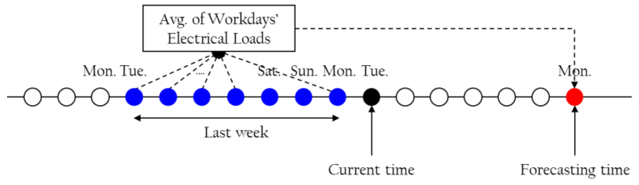
The electrical load data from the past form one of the perfect clues for forecasting the power consumption of the future and the power consumption pattern relies on the day of the week, workday, and holiday. Hence, it is necessary to consider many cases to show the electrical load of the past in the short-term load forecasting. For instance, if the prediction time is a holiday and the same day in the previous week was a workday, then their electrical loads can be very different. Therefore, it would be better to calculate the week-ahead load at the prediction time not by the electrical load data of the coming week, but by averaging the electrical loads of the days of the same type in the previous week. Thus, if the prediction time is a workday, we use the average electrical load of all workdays of the previous week as an independent variable. Likewise, if the prediction time is a holiday, we use the average electrical load of all holidays of the previous week. In this way, we reflect the different electrical load characteristics of the holiday and workday in the forecasting. Figure 2 shows an example of estimating the week-ahead consumption. If the current time is Tuesday, we already know the electrical load of yesterday (Monday). Hence, to estimate the week-ahead consumption of the coming Monday, we use the average of the electrical loads of workdays of the last week.
3.2.3. Estimating the Year-Ahead Consumption
The year-ahead load aims to utilize the trend of the annual electrical load by showing the power consumption of the same week of the previous year. However, the electrical load of the exact same week of the previous year is not always used because the days of the week are different and popular Korean holidays are celebrated according to the lunar calendar. Every week of the year has a unique week number based on ISO-8601 [32]. As mentioned before, the average of power consumptions of all holidays or workdays of the week are calculated to which the prediction time belongs and depending on the year, one year comprises 52 or 53 weeks. In the case of an issue such as the prediction time belongs to the 53rd week, there is no same week number in the previous year. To solve this problem, the power consumption of the 52nd week from the previous year is utilized since the two weeks have similar external factors. Especially, electrical loads show very low consumption on a special holiday like the Lunar New Year holidays and Korean Thanksgiving days [35]. To show this usage pattern, the average power consumption of the previous year’s special holiday represents the year-ahead’s special holiday’s load. The week number can differ depending on the year, so representing the year-ahead’s special holiday power consumption cannot be done directly using the week number of the holiday. This issue can be handled easily by exchanging the power consumption of the week and the week of the holiday in the previous year. Figure 3 shows an example of estimating the year-ahead consumption. If the current time is Monday of the 33rd week 2016, we use the 33rd week’s electrical load of the last year. To estimate the year-ahead consumption of Sunday of the 33rd week, we use the average of the electrical loads of the holidays of the 33rd week of the last year.
3.2.4. Load Forecasting Based on LSTM Networks
A recurrent neural network (RNN) is a class of ANN where connections between units form a directed graph along a sequence. Unlike a feedforward neural network (FFNN), RNNs can use their internal state or memory to process input sequences [36]. RNNs can handle time series data in many applications, such as unsegmented, connected handwriting recognition or speech recognition [37]. However, RNNs have problems in that the gradient can be extremely small or large; these problems are called the vanishing gradient and exploding gradient problems. If the gradient is extremely small, RNNs cannot learn data with long-term dependencies. On the other hand, if the gradient is extremely large, it moves the RNN parameters far away and disrupts the learning process. To handle the vanishing gradient problem, previous studies [38,39] have proposed sophisticated models of RNN architectures. One successful model is long short-term memory (LSTM), which solves the RNN problem through a cell state and a unit called a cell with multiple gates. LSTM Networks use a method that influences the behind data by reflecting the learned information with the previous data as the learning progresses with time. Therefore, it is suitable for time series data, such as electrical load data. However, the LSTM networks can reflect yesterday’s information for the next day’s forecast. Since the daily load forecasting of a smart grid aims to be scheduled until after a week, LSTM networks are not suitable for application to the daily load forecasting because there is a gap of six days. Furthermore, if the prediction is not valid, the LSTM model method can give a bad result. For instance, national holidays, quick climate change, and unexpected institution-related events can produce unexpected power consumption. Therefore, the LSTM model alone is not enough for short-term load forecasting due to its simple structure and weakness in volatility. Eventually, a similar life pattern can be observed depending on the day of the week, which in return gives a similar electrical load pattern. This study uses the LSTM networks method to show the repeating pattern of power consumptions depending on the day of the week. The input variable period of the training dataset is composed of the electrical load from 2012 to 2015 and the dependent variable of the training set is composed of the electrical load from 2013 to 2015. We performed 10-fold cross-validation on a rolling basis for optimal hyper-parameter detection.
3.3. Discovering Similar Time series Patterns
So far, diverse machine learning algorithms have been proposed to predict electrical load [1,3,6,14]. However, they showed different prediction performances depending on the various factors. For instance, for time series data, one algorithm gives the best prediction performance on one segment, while for other segments, another algorithm can give the best performance. Hence, one way to improve the accuracy in this case is to use more than one predictive algorithm. We consider electrical load data as time series data and utilize a decision tree to classify the electrical load data by pattern similarity. Decision trees [26,40] can handle both categorical and numerical data, and are highly persuasive because they can be analyzed through each branch of the tree, which represents the process of classification or prediction. In addition, they exhibit a high explanatory power because they can confirm which independent variables have a higher impact when predicting the value of a dependent or target variable. On the other hand, continuous variables used in the prediction of values of the time series are regarded as discontinuous values, and hence, the prediction errors are likely to occur near the boundary of separation. Hence, using the decision tree, we divide continuous dependent variables into several classes with a similar electrical load pattern. To do this, we use the training dataset from the previous three years. We use the daily electrical load as the attribute of class label or dependent variable and the characteristics of the time series as independent variables, representing year, month, day, day of the week, holiday, and academic year. Details on the classification of time series data will be shown in the experimental section.
3.4. Building a Hybrid Forecasting Model
To construct our hybrid prediction model, we combine both a random forest model and multilayer perceptron model. Random forest is a representative ensemble model, while MLP is a representative deep learning model; both these models have shown an excellent performance in forecasting electrical load [5,12,15,16,17].
Random forest [41,42] is an ensemble method for classification, regression, and other tasks. It constructs many decision trees that can be used to classify a new instance by the majority vote. Each decision tree node uses a subset of attributes randomly selected from the original set of attributes. Random forest runs efficiently on large amounts of data and provides a high accuracy [43]. In addition, compared to other machine learning algorithms such as ANN and SVR, it requires less fine-tuning of its hyper-parameters [16]. The basic parameters of random forest include the total number of trees to be generated (nTree) and the decision tree-related parameters (mTry), such as minimum split and split criteria [17]. In this study, we find the optimal mTry and nTree for our forecasting model by using the training set and then verify their performance using the validation and test set. The authors in [42] suggested that a random forest should have 64 to 128 trees and we use 128 trees for our hybrid STLF model. In addition, the mTry values used for this study provided by scikit-learn are as follows.
- Auto: max features = n features.
- Sqrt: max features = sqrt (n features).
- Log2: max features = log2 (n features).
A typical ANN architecture, known as a multilayer perceptron, is a type of machine learning algorithm that is a network of individual nodes, called perceptrons, organized in a series of layers [5]. Each layer in MLP is categorized into three types: an input layer, which receives features used for prediction; a hidden layer, where hidden features are extracted; and an output layer, which yields the determined results. Among them, the hidden layer has many factors affecting performance, such as the number of layers, the number of nodes involved, and the activation function of the node [44]. Therefore, the network performance depends on how the hidden layer is configured. In particular, the number of hidden layers determines the depth or shallowness of the network. In addition, if there are more than two hidden layers, it is called a deep neural network (DNN) [45]. To establish our MLP, we use two hidden layers since we do not require many input variables in our prediction model. In addition, we use the same epochs and batch size as the LSTM model we described previously. Furthermore, as an activation function, we use an exponential linear unit (ELU) without the rectified linear unit (ReLU), which has gained increasing popularity recently. However, its main disadvantage is that the perceptron can die in the learning process. ELU [46] is an approximate function introduced to overcome this disadvantage, and can be defined by:
The next important consideration is to choose the number of hidden nodes. Many studies have been conducted to determine the optimal number of hidden nodes for a given task [15,47,48], and we decided to use two different hidden node counts: the number of input variables and 2/3 of the number of input variables. Since we use nine input variables, the numbers of hidden nodes we will use are 9 and 6. Since our model has two hidden layers, we can consider three configurations, depending on the hidden nodes of the first and second layers: (9, 9), (9, 6), and (6, 6). As in the random forest, we evaluate these configurations using the training data for each building cluster and identify the configuration that gives the best prediction accuracy. After that, we compare the best MLP model with the random forest model for each cluster type.
3.5. Time series Cross-Validation
To construct a forecasting model, the dataset is usually divided into a training set and test set. Then, the training set is used in building a forecasting model and the test set is used in evaluating the resulting model. However, in traditional time series forecasting techniques, the prediction performance is poorer as the interval between the training and forecasting times increases. To alleviate this problem, we apply the time series cross-validation (TSCV) based on the rolling forecasting origin [49]. A variation of this approach focuses on a single prediction horizon for each test set. In this approach, we use various training sets, each containing one extra observation than the previous one. We calculate the prediction accuracy by first measuring the accuracy for each test set and then averaging the results of all test sets. This paper proposes a one-week (sum from 145 h to 168 h) look-ahead view of the operation for smart grids. For this, a seven-step-ahead forecasting model is built to forecast the power consumption at a single time (h + 7 + i − 1) using the test set with observations at several times (1, 2, …, h + i − 1). If h observations are required to produce a reliable forecast, then, for the total T observations, the process works as follows.
For i = 1 to T − h − 6:
- (1)
- Select the observation at time h + 7 + i − 1 for the test set;
- (2)
- Consider the observations at several times 1, 2, ⋯, h + i − 1 to estimate the forecasting model;
- (3)
- Calculate the 7-step error on the forecast for time h + 7 + i − 1;
- (4)
- Compute the forecast accuracy based on the errors obtained.
4. Performance Metrics
To analyze the forecast model performance, several metrics, such as mean absolute percentage error (MAPE), root mean square error (RMSE), and mean absolute error (MAE), are used, which are well-known for representing the prediction accuracy.
4.1. Mean Absolute Percentage Error
MAPE is a measure of prediction accuracy for constructing fitted time series values in statistics, specifically in trend estimation. It usually presents accuracy as a percentage of the error and can be easier to comprehend than the other statistics since this number is a percentage. It is known that the MAPE is huge if the actual value is very close to zero. However, in this work, we do not have such values. The formula for MAPE is shown in Equation (3), where and are the actual and forecast values, respectively. In addition, is the number of times observed.
4.2. Root Mean Square Error
RMSE (also called the root mean square deviation, RMSD) is used to aggregate the residuals into a single measure of predictive ability. The square root of the mean square error, as shown in Equation (4), is the forecast value and an actual value . The mean square standard deviation of the forecast value for the actual value is the square root of RMSE. For an unbiased estimator, RMSE is the square root of the variance, which denotes the standard error.
4.3. Mean Absolute Error
In statistics, MAE is used to evaluate how close forecasts or predictions are to the actual outcomes. It is calculated by averaging the absolute differences between the prediction values and the actual observed values. MAE is defined as shown in Equation (5), where is the forecast value and is the actual value.
5. Experimental Results
To evaluate the performance of our hybrid forecast model, we carried out several experiments. We performed preprocessing for the dataset in the Python environment and performed forecast modeling using scikit-learn [50], TensorFlow [51], and Keras [52]. We used six years of daily electrical load data from 2012 to 2017. Specifically, we used electrical load data of 2012 to configure input variables for a training set. Data from 2013 to 2015 was used as the training set, the data of 2016 was the validation set, and the data of 2017 was the test set.
5.1. Dataset Description
Table 2 shows the statistics of the electric consumption data for each cluster, including the number of valid cases, mean, and standard deviation. As shown in the table, Cluster B has a higher power consumption and wider deviation than clusters A and C.
5.2. Forecasting Model Configuration
In this study, we used the LSTM networks method to show the repeating pattern of power consumptions depending on the day of the week. We tested diverse cases and investigated the accuracy of load forecasting for the test cases to determine the best input data selection. As shown in Figure 4, the input variables consist of four electrical loads from one week ago to four weeks ago as apart at a weekly interval to reflect the cycle of one month. In the feature scaling process, we rescaled the range of the measured values from 0 to 1. We used tanh as the activation function and calculated the loss by using the mean absolute error. We used the adaptive moment estimation (Adam) method, which combines momentum and root mean square propagation (RMSProp), as the optimization method. The Adam optimization technique weighs the time series data and maintains the relative size difference between the variables. In the configuration of the remaining hyper-parameters of the model, we set the number of hidden units to 60, epochs to 300, and batch size to 12.
We experimented with the LSTM model [52] by changing the time step from one cycle to a maximum of 30 cycles. Table 3 shows the mean absolute percentage error (MAPE) of each cluster for each time step. In the table, the predicted results with the best accuracy are marked in bold. Table 3 shows that the 27th time step indicates the most accurate prediction performance. In general, the electricity demand is relatively high in summer and winter, compared to that in spring and autumn. In other words, it has a rise and fall curve in a half-year cycle, and the 27th time step corresponds to a week number of about half a year.
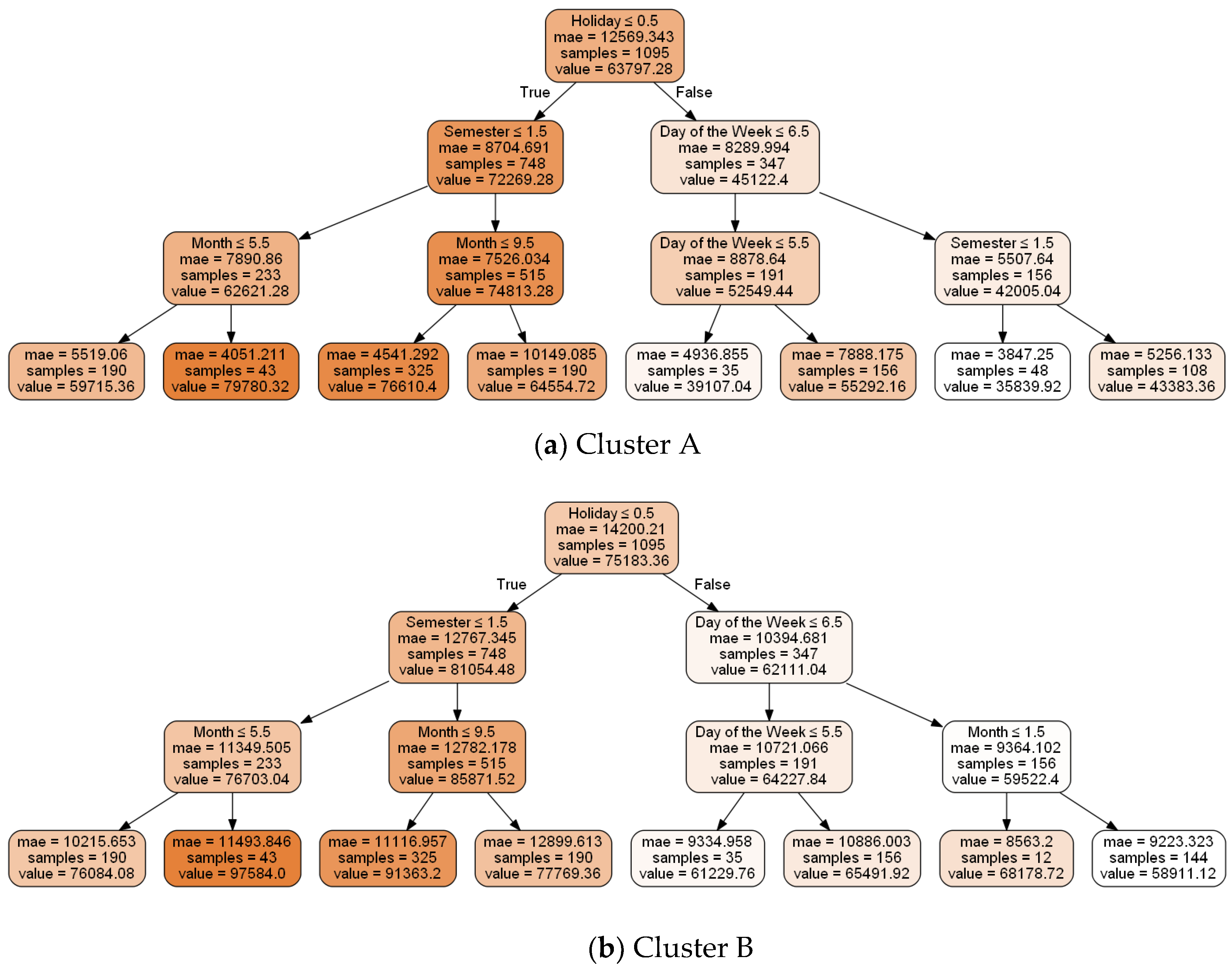
We performed similar a time series pattern analysis based on the decision tree through 10-fold cross-validation for the training set. Among several options provided by scikit-learn to construct a decision tree, we considered the criterion, max depth, and max features. The criterion is a function for measuring the quality of a split. In this paper, we use the “mae” criterion for our forecasting model since it gives the smallest error rate between the actual and the classification value. Max depth is the maximum depth of the tree. We set max depth to 3, such that the number of leaves is 8. In other words, the decision tree classifies the training datasets into eight similar time series. Max features are the number of features to consider when looking for the best split. We have chosen the “auto” option to reflect all time variables. Figure 5 shows the result of the similar time series recognition for each cluster using the decision tree. Here, samples indicate the number of tuples in each leaf. The total number of samples is 1095, since we are considering the daily consumption data over three years. Value denotes the classification value of the similar time series. Table 4 shows the number of similar time series samples according to the decision tree for 2016 and 2017.
The predictive evaluation consists of two steps. Based on the forecast models of random forest and MLP, we used the training set from 2013 to 2015 and predicted the verification period of 2016. The objectives are to detect models with optimal hyper-parameters and then to select models with a better predictive performance in similar time series. Next, we set the training set to include data from 2013 to 2016 and predicted the test period of 2017. Here, we evaluate the predictive performance of the hybrid model we have constructed. Table 5 is the prediction result composed of MLP, and MAPE is used as a measure of prediction accuracy and the predicted results with the best accuracy are marked in bold. As shown in the table, overall, a model consisting of nine and nine nodes in each hidden layer showed the best performance. Although the nine and six nodes in each hidden layer showed a better performance in Cluster A, the model consisting of nine and nine nodes was selected to generalize the predictive model.
Table 6 shows the MAPE of random forest for each cluster under different mTry and the predicted results with the best accuracy are marked in bold. Since the input variable is 9, sqrt and log2 are recognized as 3 and the results are the same. We choose the sqrt that is commonly used [16,43].
Figure 6a–c show the use of forests of trees to evaluate the importance of features in an artificial classification task. The blue bars denote the feature importance of the forest, along with their inter-trees variability. In the figure, LSTM, which refers to the LSTM-RNN that reflects the trend of day of the week, has the highest impact on the model configuration for all clusters. Other features have different impacts, depending on the cluster type.
Table 7 shows the electrical load forecast accuracy for the pattern classification of similar time series for 2016. In the table, the predicted results with a better accuracy are marked in bold. For instance, in the case of Cluster A, while random forest shows a better prediction accuracy for patterns 1 to 4, MLP shows a better accuracy for patterns 5 to 8. Using this table, we can choose a more accurate prediction model for the pattern and cluster type.
Table 8 shows prediction results of our model for 2017. Comparing Table 7 and Table 8, we can see that MLP and random forest (RF) have a matched relative performance in most cases. There are two exceptions in Cluster A and one exception in Cluster B and they are underlined and marked in bold. In the case of Cluster C, MLP and RF gave the same relative performance. This is good evidence that our hybrid model can be generalized.
5.3. Comparison of Forecasting Techniques
To verify the validness and applicability of our hybrid daily load forecasting model, the predictive performance of our model should be compared with other machine learning techniques, including ANN and SVR, which are very popular predictive techniques [6]. In this comparison, we consider eight models, including our model, as shown in Table 9. In the table, GBM (Gradient Boosting Machine) is a type of ensemble learning technique that implements the sequential boosting algorithm. A grid search can be used to find optimal hyper-parameter values for the SVR/GBM [25]. SNN (Shallow Neural Network) has three layers of input, hidden, and output, and it was found that the optimal number of the hidden nodes is nine for all clusters.
Table 9, Table 10 and Table 11 compare the prediction performance in terms of MAPE, RMSE, and MAE, respectively. From the tables, the predicted results with the best accuracy are marked in bold and we observe that our hybrid model exhibits a superb performance in all categories. Figure 7 shows more detail of the MAPE distribution for each cluster using a box plot. We can deduce that our hybrid model has fewer outliers and a smaller maximum error. In addition, the error rate increases in the case of long holidays in Korea. For instance, during the 10-day holiday in October 2017, the error rate increased significantly. Another cause of high error rates is due to outliers or missing values because of diverse reasons, such as malfunction and surge. Figure 8 compares the daily load forecasts of our hybrid model and actual daily usage on a quarterly basis. Overall, our hybrid model showed a good performance in predictions, regardless of diverse external factors such as long holidays.
Nevertheless, we can see that there are several time periods when forecasting errors are high. For instance, from 2013 to 2016, Cluster B showed a steady increase in its power consumption due to building remodeling and construction. Even though the remodeling and construction are finished at the beginning of 2017, the input variable for estimating the year-ahead consumption is still reflecting such an increase. This was eventually adjusted properly for the third and fourth quarters by the time series cross-validation. On the other hand, during the remodeling, the old heating, ventilation, and air conditioning (HVAC) system was replaced by a much more efficient one and the new system started its operation in December 2017. Even though our hybrid model predicted much higher power consumption for the cold weather in the third week, the actual power consumption was quite low due to the new HVAC system. Lastly, Cluster A showed a high forecasting error on 29 November 2017. It turned out that at that time, there were several missing values in the actual power consumption. This kind of problem can be detected by using the outlier detection technique.
6. Conclusions
In this paper, we proposed a hybrid model for short-term load forecasting for higher educational institutions, such as universities, using random forest and multilayer perceptron. To construct our forecast model, we first grouped university buildings into an academic cluster, science/engineering cluster, and dormitory cluster, and collected their daily electrical load data over six years. We divided the collected data into a training set, a validation set, and a test set. For the training set, we classified electrical load data by pattern similarity using the decision tree technique. We considered various configurations for random forest and multilayer perceptron and evaluated their prediction performance by using the validation set to select the optimal model. Based on this work, we constructed our hybrid daily electrical load forecast model by selecting models with a better predictive performance in similar time series. Finally, using the test set, we compared the daily electrical load prediction performance of our hybrid model and other popular models. The comparison results show that our hybrid model outperforms other popular models. In conclusion, we showed that LSTM networks are effective for reflecting an electrical load depending on the day of the week and the decision tree is effective in classifying time series data by similarity. Moreover, using these two forecasting models in a hybrid model can complement their weaknesses.
In order to improve the accuracy of electrical load prediction, we plan to use a supervised learning method reflecting various statistically significant data. Also, we will analyze the prediction performance in different look-ahead points (from the next day to a week) using probabilistic forecasting.
Author Contributions
J.M. designed the algorithm, performed the simulations, and prepared the manuscript as the first author. Y.K. analyzed the data and visualized the experimental results. M.S. collected the data, and developed and wrote the load forecasting based on the LSTM networks part. E.H. conceived and supervised the work. All authors discussed the simulation results and approved the publication.
Funding
This research was supported by Korea Electric Power Corporation (Grant number: R18XA05) and the Brain Korea 21 Plus Project in 2018.
Conflicts of Interest
The authors declare no conflict of interest.
References
- Lindley, D. Smart grids: The energy storage problem. Nat. News 2010, 463, 18–20. [Google Scholar] [CrossRef] [PubMed] [Green Version]
- Erol-Kantarci, M.; Mouftah, H.T. Energy-efficient information and communication infrastructures in the smart grid: A survey on interactions and open issues. IEEE Commun. Surv. Tutor. 2015, 17, 179–197. [Google Scholar] [CrossRef]
- Raza, M.Q.; Khosravi, A. A review on artificial intelligence based load demand forecasting techniques for smart grid and buildings. Renew. Sustain. Energy Rev. 2015, 50, 1352–1372. [Google Scholar] [CrossRef]
- Hernandez, L.; Baladron, C.; Aguiar, J.M.; Carro, B.; Sanchez-Esguevillas, A.J.; Lloret, J.; Massana, J. A survey on electric power demand forecasting: Future trends in smart grids, microgrids and smart buildings. IEEE Commun. Surv. Tutor. 2014, 16, 1460–1495. [Google Scholar] [CrossRef]
- Kuo, P.-H.; Huang, C.-J. A High Precision Artificial Neural Networks Model for Short-Term Energy Load Forecasting. Energies 2018, 11, 213. [Google Scholar] [CrossRef]
- Ahmad, A.; Hassan, M.; Abdullah, M.; Rahman, H.; Hussin, F.; Abdullah, H.; Saidur, R. A review on applications of ANN and SVM for building electrical energy consumption forecasting. Renew. Sustain. Energy Rev. 2014, 33, 102–109. [Google Scholar] [CrossRef]
- Vrablecová, P.; Ezzeddine, A.B.; Rozinajová, V.; Šárik, S.; Sangaiah, A.K. Smart grid load forecasting using online support vector regression. Comput. Electr. Eng. 2017, 65, 102–117. [Google Scholar] [CrossRef]
- Hong, T.; Fan, S. Probabilistic electric load forecasting: A tutorial review. Int. J. Forecast. 2016, 32, 914–938. [Google Scholar] [CrossRef]
- Hahn, H.; Meyer-Nieberg, S.; Pickl, S. Electric load forecasting methods: Tools for decision making. Eur. J. Oper. Res. 2009, 199, 902–907. [Google Scholar] [CrossRef]
- Moon, J.; Park, J.; Hwang, E.; Jun, S. Forecasting power consumption for higher educational institutions based on machine learning. J. Supercomput. 2018, 74, 3778–3800. [Google Scholar] [CrossRef]
- Chung, M.H.; Rhee, E.K. Potential opportunities for energy conservation in existing buildings on university campus: A field survey in Korea. Energy Build. 2014, 78, 176–182. [Google Scholar] [CrossRef]
- Moon, J.; Kim, K.-H.; Kim, Y.; Hwang, E. A Short-Term Electric Load Forecasting Scheme Using 2-Stage Predictive Analytics. In Proceedings of the IEEE International Conference on Big Data and Smart Computing (BigComp), Shanghai, China, 15–17 January 2018; pp. 219–226. [Google Scholar]
- Palchak, D.; Suryanarayanan, S.; Zimmerle, D. An Artificial Neural Network in Short-Term Electrical Load Forecasting of a University Campus: A Case Study. J. Energy Resour. Technol. 2013, 135, 032001. [Google Scholar] [CrossRef]
- Wang, Z.; Srinivasan, R.S. A review of artificial intelligence based building energy use prediction: Contrasting the capabilities of single and ensemble prediction models. Renew. Sustain. Energy Rev. 2016, 75, 796–808. [Google Scholar] [CrossRef]
- Hippert, H.S.; Pedreira, C.E.; Souza, R.C. Neural networks for short-term load forecasting: A review and evaluation. IEEE Trans. Power Syst. 2001, 16, 44–55. [Google Scholar] [CrossRef]
- Lahouar, A.; Slama, J.B.H. Day-ahead load forecast using random forest and expert input selection. Energy Convers. Manag. 2015, 103, 1040–1051. [Google Scholar] [CrossRef]
- Ahmad, M.W.; Mourshed, M.; Rezgui, Y. Trees vs Neurons: Comparison between random forest and ANN for high-resolution prediction of building energy consumption. Energy Build. 2017, 147, 77–89. [Google Scholar] [CrossRef]
- Xiao, L.; Wang, J.; Dong, Y.; Wu, J. Combined forecasting models for wind energy forecasting: A case study in China. Renew. Sustain. Energy Rev. 2015, 44, 271–288. [Google Scholar] [CrossRef]
- Pinson, P.; Kariniotakis, G. Conditional prediction intervals of wind power generation. IEEE Trans. Power Syst. 2010, 25, 1845–1856. [Google Scholar] [CrossRef] [Green Version]
- Abdoos, A.; Hemmati, M.; Abdoos, A.A. Short term load forecasting using a hybrid intelligent method. Knowl. Based Syst. 2015, 76, 139–147. [Google Scholar] [CrossRef]
- Dong, J.-r.; Zheng, C.-y.; Kan, G.-y.; Zhao, M.; Wen, J.; Yu, J. Applying the ensemble artificial neural network-based hybrid data-driven model to daily total load forecasting. Neural Comput. Appl. 2015, 26, 603–611. [Google Scholar] [CrossRef]
- Lee, W.-J.; Hong, J. A hybrid dynamic and fuzzy time series model for mid-term power load forecasting. Int. J. Electr. Power. Energy Syst. 2015, 64, 1057–1062. [Google Scholar] [CrossRef]
- Zhang, T.; Wang, J. K-nearest neighbors and a kernel density estimator for GEFCom2014 probabilistic wind power forecasting. Int. J. Forecast. 2016, 32, 1074–1080. [Google Scholar] [CrossRef]
- Jurado, S.; Nebot, À.; Mugica, F.; Avellana, N. Hybrid methodologies for electricity load forecasting: Entropy-based feature selection with machine learning and soft computing techniques. Energy 2015, 86, 276–291. [Google Scholar] [CrossRef] [Green Version]
- Feng, C.; Cui, M.; Hodge, B.-M.; Zhang, J. A data-driven multi-model methodology with deep feature selection for short-term wind forecasting. Appl. Energy 2017, 190, 1245–1257. [Google Scholar] [CrossRef]
- Tso, G.K.; Yau, K.K. Predicting electricity energy consumption: A comparison of regression analysis, decision tree and neural networks. Energy 2007, 32, 1761–1768. [Google Scholar] [CrossRef]
- Jain, R.K.; Smith, K.M.; Culligan, P.J.; Taylor, J.E. Forecasting energy consumption of multi-family residential buildings using support vector regression: Investigating the impact of temporal and spatial monitoring granularity on performance accuracy. Appl. Energy 2014, 123, 168–178. [Google Scholar] [CrossRef]
- Grolinger, K.; L’Heureux, A.; Capretz, M.A.; Seewald, L. Energy forecasting for event venues: Big data and prediction accuracy. Energy Build. 2016, 112, 222–233. [Google Scholar] [CrossRef]
- Amber, K.; Aslam, M.; Hussain, S. Electricity consumption forecasting models for administration buildings of the UK higher education sector. Energy Build. 2015, 90, 127–136. [Google Scholar] [CrossRef]
- Rodrigues, F.; Cardeira, C.; Calado, J.M.F. The daily and hourly energy consumption and load forecasting using artificial neural network method: A case study using a set of 93 households in Portugal. Energy 2014, 62, 220–229. [Google Scholar] [CrossRef]
- Efendi, R.; Ismail, Z.; Deris, M.M. A new linguistic out-sample approach of fuzzy time series for daily forecasting of Malaysian electricity load demand. Appl. Soft Comput. 2015, 28, 422–430. [Google Scholar] [CrossRef]
- ISO Week Date. Available online: https://en.wikipedia.org/wiki/ISO_week_date (accessed on 19 October 2018).
- Holidays and Observances in South Korea in 2017. Available online: https://www.timeanddate.com/holidays/south-korea/ (accessed on 28 April 2018).
- Climate of Seoul. Available online: https://en.wikipedia.org/wiki/Climate_of_Seoul (accessed on 28 April 2018).
- Son, S.-Y.; Lee, S.-H.; Chung, K.; Lim, J.S. Feature selection for daily peak load forecasting using a neuro-fuzzy system. Multimed. Tools Appl. 2015, 74, 2321–2336. [Google Scholar] [CrossRef]
- Kong, W.; Dong, Z.Y.; Jia, Y.; Hill, D.J.; Xu, Y.; Zhang, Y. Short-term residential load forecasting based on LSTM recurrent neural network. IEEE Trans. Smart Grid 2017. [Google Scholar] [CrossRef]
- Kanai, S.; Fujiwara, Y.; Iwamura, S. Preventing Gradient Explosions in Gated Recurrent Units. In Proceedings of the Neural Information Processing Systems, Long Beach, CA, USA, 4–9 December 2017; pp. 435–444. [Google Scholar]
- Cho, K.; van Merriënboer, B.; Gulcehre, C.; Bahdanau, D.; Bougares, F.; Schwenk, H.; Bengio, Y. Learning phrase representations using RNN encoder-decoder for statistical machine translation. arXiv, 2014; arXiv:1406.1078. [Google Scholar]
- Hochreiter, S.; Schmidhuber, J. Long short-term memory. Neural Comput. 1997, 9, 1735–1780. [Google Scholar] [CrossRef] [PubMed]
- Rutkowski, L.; Jaworski, M.; Pietruczuk, L.; Duda, P. The CART decision tree for mining data streams. Inf. Sci. 2014, 266, 1–15. [Google Scholar] [CrossRef]
- Breiman, L. Random forests. Mach. Learn. 2001, 45, 5–32. [Google Scholar] [CrossRef]
- Oshiro, T.M.; Perez, P.S.; Baranauskas, J.A. How many trees in a random forest? In Proceedings of the International Conference on Machine Learning and Data Mining in Pattern Recognition, Berlin, Germany, 13–20 July 2012; pp. 154–168. [Google Scholar]
- Díaz-Uriarte, R.; De Andres, S.A. Gene selection and classification of microarray data using random forest. BMC Bioinform. 2006, 7, 3. [Google Scholar] [CrossRef] [PubMed] [Green Version]
- Suliman, A.; Zhang, Y. A Review on Back-Propagation Neural Networks in the Application of Remote Sensing Image Classification. J. Earth Sci. Eng. (JEASE) 2015, 5, 52–65. [Google Scholar] [CrossRef]
- Bengio, Y. Learning deep architectures for AI. Found. Trends® Mach. Learn. 2009, 2, 1–127. [Google Scholar] [CrossRef]
- Clevert, D.-A.; Unterthiner, T.; Hochreiter, S. Fast and accurate deep network learning by exponential linear units (elus). arXiv, 2015; arXiv:1511.07289. [Google Scholar]
- Sheela, K.G.; Deepa, S.N. Review on methods to fix number of hidden neurons in neural networks. Math. Probl. Eng. 2013, 425740. [Google Scholar] [CrossRef]
- Xu, S.; Chen, L. A novel approach for determining the optimal number of hidden layer neurons for FNN’s and its application in data mining. In Proceedings of the 5th International Conference on Information Technology and Application (ICITA), Cairns, Australia, 23–26 June 2008; pp. 683–686. [Google Scholar]
- Hyndman, R.J.; Athanasopoulos, G. Forecasting: Principles and Practice; Otexts: Melbourne, Australia, 2014; ISBN 0987507117. [Google Scholar]
- Pedregosa, F.; Varoquaux, G.; Gramfort, A.; Michel, V.; Thirion, B.; Grisel, O.; Blondel, M.; Prettenhofer, P.; Weiss, R.; Dubourg, V. Scikit-learn: Machine learning in Python. J. Mach. Learn. Res. 2011, 12, 2825–2830. [Google Scholar]
- Abadi, M.; Barham, P.; Chen, J.; Chen, Z.; Davis, A.; Dean, J.; Devin, M.; Ghemawat, S.; Irving, G.; Isard, M. TensorFlow: A System for Large-Scale Machine Learning. In Proceedings of the 12th USENIX Symposium on Operating Systems Design and Implementation (OSDI ’16), Savannah, GA, USA, 2–4 November 2016; pp. 265–283. [Google Scholar]
- Ketkar, N. Introduction to Keras. In Deep Learning with Python; Apress: Berkeley, CA, USA, 2017; pp. 97–111. [Google Scholar]
Figure 1.
Our framework for hybrid daily electrical load forecasting.

Figure 2.
Example of estimating week-ahead consumption.

Figure 3.
Example of estimating the year-ahead consumption.

Figure 4.
System architecture of LSTM networks.

Figure 5.
Results of similar time series classifications using decision trees.


Figure 6.
Feature importance in random forest.


Figure 7.
Distribution of each model by MAPE.

Figure 8.
Daily electrical load forecasting for university campus.


Table 1.
Comparison of Pearson correlation coefficients.
| Temperature Type | Cluster # | ||
|---|---|---|---|
| Cluster A | Cluster B | Cluster C | |
| Minimum temperature | −0.018 | 0.101 | 0.020 |
| Maximum temperature | −0.068 | 0.041 | −0.06 |
| Average temperature | −0.043 | 0.072 | −0.018 |
| Adjusted temperature | 0.551 | 0.425 | 0.504 |
Table 2.
Statistics of power consumption data.
| Statistics | Cluster # | ||
|---|---|---|---|
| Cluster A | Cluster B | Cluster C | |
| Number of valid cases | 1826 | 1826 | 1826 |
| Mean | 63,094.97 | 68,860.93 | 30,472.31 |
| Variance | 246,836,473 | 269,528,278 | 32,820,509 |
| Standard deviation | 15,711.03 | 16,417.31 | 5728.92 |
| Maximum | 100,222.56 | 109,595.52 | 46,641.6 |
| Minimum | 23,617.92 | 26,417.76 | 14,330.88 |
| Lower quartile | 52,202.4 | 56,678.88 | 26,288.82 |
| Median | 63,946.32 | 66,996.72 | 30,343.14 |
| Upper quartile | 76,386.24 | 79,209.96 | 34,719.45 |
Table 3.
MAPE results of LSTM networks.
| Time Step | Cluster A | Cluster B | Cluster C | Average |
|---|---|---|---|---|
| 1 | 9.587 | 6.989 | 6.834 | 7.803 |
| 2 | 9.169 | 6.839 | 6.626 | 7.545 |
| 3 | 8.820 | 6.812 | 6.463 | 7.365 |
| 4 | 8.773 | 6.750 | 6.328 | 7.284 |
| 5 | 8.686 | 6.626 | 6.191 | 7.168 |
| 6 | 8.403 | 6.695 | 5.995 | 7.031 |
| 7 | 8.405 | 6.700 | 6.104 | 7.070 |
| 8 | 8.263 | 6.406 | 5.846 | 6.839 |
| 9 | 8.260 | 6.583 | 5.648 | 6.830 |
| 10 | 8.286 | 6.318 | 5.524 | 6.709 |
| 11 | 8.095 | 6.438 | 5.666 | 6.733 |
| 12 | 8.133 | 6.469 | 5.917 | 6.840 |
| 13 | 7.715 | 6.346 | 5.699 | 6.587 |
| 14 | 7.770 | 6.263 | 5.399 | 6.477 |
| 15 | 7.751 | 6.139 | 5.306 | 6.399 |
| 16 | 7.561 | 5.974 | 5.315 | 6.283 |
| 17 | 7.411 | 5.891 | 5.450 | 6.251 |
| 18 | 7.364 | 6.063 | 5.398 | 6.275 |
| 19 | 7.466 | 6.089 | 5.639 | 6.398 |
| 20 | 7.510 | 5.892 | 5.627 | 6.343 |
| 21 | 7.763 | 5.977 | 5.451 | 6.397 |
| 22 | 7.385 | 5.856 | 5.460 | 6.234 |
| 23 | 7.431 | 5.795 | 5.756 | 6.327 |
| 24 | 7.870 | 6.089 | 5.600 | 6.520 |
| 25 | 7.352 | 5.923 | 5.370 | 6.215 |
| 26 | 7.335 | 5.997 | 5.285 | 6.206 |
| 27 | 7.405 | 5.479 | 5.371 | 6.085 |
| 28 | 7.422 | 5.853 | 5.128 | 6.134 |
| 29 | 7.553 | 5.979 | 5.567 | 6.366 |
| 30 | 7.569 | 5.601 | 5.574 | 6.248 |
Table 4.
Similar time series patterns.
| Pattern | Cluster A | Cluster B | Cluster C | |||
|---|---|---|---|---|---|---|
| 2016 | 2017 | 2016 | 2017 | 2016 | 2017 | |
| 1 | 62 | 62 | 62 | 62 | 62 | 62 |
| 2 | 14 | 14 | 14 | 14 | 140 | 138 |
| 3 | 107 | 111 | 107 | 111 | 20 | 20 |
| 4 | 64 | 58 | 64 | 58 | 25 | 25 |
| 5 | 14 | 15 | 14 | 15 | 1 | 2 |
| 6 | 53 | 52 | 53 | 52 | 10 | 9 |
| 7 | 16 | 16 | 5 | 5 | 99 | 98 |
| 8 | 36 | 37 | 47 | 48 | 9 | 11 |
| Total | 366 | 365 | 366 | 365 | 366 | 365 |
Table 5.
MAPE results of the multilayer perceptron.
| Cluster # | Number of Neurons in Each Layer | ||
|---|---|---|---|
| 9-6-6-1 | 9-9-6-1 | 9-9-9-1 | |
| Cluster A | 3.856 | 3.767 | 3.936 |
| Cluster B | 4.869 | 5.076 | 4.424 |
| Cluster C | 3.366 | 3.390 | 3.205 |
Table 6.
MAPE results of random forest.
| Cluster # | Number of Features | ||
|---|---|---|---|
| Auto | sqrt | log2 | |
| Cluster A | 3.983 | 3.945 | 3.945 |
| Cluster B | 4.900 | 4.684 | 4.684 |
| Cluster C | 3.579 | 3.266 | 3.266 |
Table 7.
MAPE results of load forecasting in 2016.
| 2016 | Cluster A | Cluster B | Cluster C | |||
|---|---|---|---|---|---|---|
| Pattern | MLP | RF | MLP | RF | MLP | RF |
| 1 | 3.339 | 3.092 | 3.705 | 2.901 | 2.736 | 2.475 |
| 2 | 2.199 | 1.965 | 4.395 | 3.602 | 2.987 | 2.731 |
| 3 | 2.840 | 2.712 | 3.343 | 2.990 | 2.853 | 2.277 |
| 4 | 4.165 | 3.472 | 3.794 | 3.978 | 3.517 | 2.568 |
| 5 | 7.624 | 9.259 | 8.606 | 15.728 | 4.229 | 10.303 |
| 6 | 4.617 | 5.272 | 5.404 | 6.172 | 5.159 | 4.894 |
| 7 | 3.816 | 4.548 | 9.199 | 8.860 | 3.686 | 4.718 |
| 8 | 6.108 | 6.402 | 5.844 | 6.768 | 2.152 | 2.595 |
Table 8.
MAPE results of load forecasting in 2017.
| 2017 | Cluster A | Cluster B | Cluster C | |||
|---|---|---|---|---|---|---|
| Pattern | MLP | RF | MLP | RF | MLP | RF |
| 1 | 2.914 | 2.709 | 4.009 | 3.428 | 2.838 | 2.524 |
| 2 | 1.945 | 2.587 | 3.313 | 3.442 | 2.622 | 2.474 |
| 3 | 2.682 | 2.629 | 3.464 | 3.258 | 3.350 | 2.583 |
| 4 | 5.025 | 4.211 | 4.005 | 5.116 | 2.694 | 2.391 |
| 5 | 7.103 | 11.585 | 9.640 | 20.718 | 3.300 | 15.713 |
| 6 | 4.503 | 6.007 | 5.956 | 7.272 | 6.984 | 6.296 |
| 7 | 3.451 | 3.517 | 13.958 | 12.386 | 3.835 | 4.443 |
| 8 | 6.834 | 6.622 | 7.131 | 8.106 | 2.562 | 3.722 |
Table 9.
MAPE distribution for each forecasting model.
| Forecasting Model | Cluster # | ||
|---|---|---|---|
| Cluster A | Cluster B | Cluster C | |
| MR | 7.852 | 8.971 | 4.445 |
| DT | 6.536 | 8.683 | 6.004 |
| GBM | 4.831 | 6.896 | 3.920 |
| SVR | 4.071 | 5.761 | 3.135 |
| SNN | 4.054 | 5.948 | 3.181 |
| MLP | 3.961 | 4.872 | 3.139 |
| RF | 4.185 | 5.641 | 3.216 |
| RF+MLP | 3.798 | 4.674 | 2.946 |
Table 10.
RMSE comparison for each forecasting model.
| Forecasting Model | Cluster # | ||
|---|---|---|---|
| Cluster A | Cluster B | Cluster C | |
| MR | 5725.064 | 6847.179 | 1757.463 |
| DT | 6118.835 | 7475.188 | 2351.676 |
| GBM | 4162.359 | 5759.276 | 1495.751 |
| SVR | 3401.812 | 5702.405 | 1220.052 |
| SNN | 3456.156 | 4903.587 | 1236.606 |
| MLP | 3381.697 | 4064.559 | 1170.824 |
| RF | 4111.245 | 4675.762 | 1450.436 |
| RF + MLP | 3353.639 | 3894.495 | 1143.297 |
Table 11.
MAE comparison for each forecasting model.
| Forecasting Model | Cluster # | ||
|---|---|---|---|
| Cluster A | Cluster B | Cluster C | |
| MR | 4155.572 | 4888.821 | 1262.985 |
| DT | 3897.741 | 5054.069 | 1708.709 |
| GBM | 2764.128 | 3916.945 | 1122.530 |
| SVR | 2236.318 | 3956.907 | 898.963 |
| SNN | 2319.696 | 3469.775 | 919.014 |
| MLP | 2255.537 | 2795.246 | 910.351 |
| RF | 2708.848 | 3235.855 | 1063.731 |
| RF+MLP | 2208.072 | 2742.543 | 860.989 |
© 2018 by the authors. Licensee MDPI, Basel, Switzerland. This article is an open access article distributed under the terms and conditions of the Creative Commons Attribution (CC BY) license (http://creativecommons.org/licenses/by/4.0/).
Share and Cite
MDPI and ACS Style
Moon, J.; Kim, Y.; Son, M.; Hwang, E. Hybrid Short-Term Load Forecasting Scheme Using Random Forest and Multilayer Perceptron. Energies 2018, 11, 3283. https://doi.org/10.3390/en11123283
AMA Style
Moon J, Kim Y, Son M, Hwang E. Hybrid Short-Term Load Forecasting Scheme Using Random Forest and Multilayer Perceptron. Energies. 2018; 11(12):3283. https://doi.org/10.3390/en11123283
Chicago/Turabian StyleMoon, Jihoon, Yongsung Kim, Minjae Son, and Eenjun Hwang. 2018. "Hybrid Short-Term Load Forecasting Scheme Using Random Forest and Multilayer Perceptron" Energies 11, no. 12: 3283. https://doi.org/10.3390/en11123283
Note that from the first issue of 2016, this journal uses article numbers instead of page numbers. See further details here.