The Role of Demand Response Aggregators and the Effect of GenCos Strategic Bidding on the Flexibility of Demand

Abstract

This paper presents an interactive trading decision between an electricity market operator, generation companies (GenCos), and the aggregators having demand response (DR) capable loads. Decisions are made hierarchically. At the upper-level, an electricity market operator (EMO) aims to minimise generation supply cost considering a DR transaction cost, which is essentially the cost of load curtailment. A DR exchange operator aims to minimise this transaction cost upon receiving the DR offer from the multiple aggregators at the lower level. The solution at this level determines the optimal DR amount and the load curtailment price. The DR considers the end-user’s willingness to reduce demand. Lagrangian duality theory is used to solve the bi-level optimisation. The usefulness of the proposed market model is demonstrated on interconnection of the Pennsylvania-New Jersey-Maryland (PJM) 5-Bus benchmark power system model under several plausible cases. It is found that the peak electricity price and grid-wise operation expenses under this DR trading scheme are reduced.

1. Introduction

Demand-side management (DSM) with energy security and affordability objective has opened up new challenges and opportunities for the electricity market participants [1]. The term, DSM, was first introduced by the Electric Power Research Institute (EPRI) in the 1980s [2]. It refers to the change in the usual electricity consumption to optimized consumption by coordinating the demand response (DR) capable loads, renewable resources, on-site generation, and energy storage [3].

Specifically, a variety of demand response (DR) programs as part of the DSM initiatives have been used as potential resources to balance supply and demand, reduce operation cost, and to enhance power system efficiency [4,5]. The DR is defined as a change in electricity usages by the end-user customer from a usual consumption, in response to a changing electricity price [6,7]. It can be promoted via monetary incentives to lower energy consumption when the market prices are high [8]. The market price becomes higher because of power system network congestion and a power supply deficit [9].

Development of DR is triggered by policies, market mechanisms, and implementation frameworks. The Federal Electricity Regulatory Commission (FERC) in the USA assessed that DSM could reduce 9.2% of the peak demand, which is accounted to be 72,000 MW [10]. The ever-increasing DR potential is attributed to new and expanded programs. It urges market reformation toward end-user compensation and economic reward from DR service providers.

The DSM undertaken by the active participation of end-user customers is a key aspect of a smart power system [11,12,13,14,15,16,17,18,19,20]. In optimized consumption, peak load demand clips, and the valleys load demand fill [5]. From the grid operator perspective, the DSM measures substantially minimize the number of expensive peaking generating plants’ activation [21]. Furthermore, electricity networks become more sustainable, efficient, and secure.

The third-party aggregator as a profit-making liaising agent could be a key driver to make the DSM smarter via technology adoption and enhanced end-users’ interaction [22]. Aggregators will have to possess the necessary enabling technologies to manage varieties of the DR programs for the end-user customers while enticing them with appropriate compensation. The aggregators, in turn, receive rewards from the market operator for the cumulative DR services and help in shaping the load demand [23].

This paper proposes a DR integrated bi-level optimization framework. The bi-level optimization is a special kind of mathematical program, where an optimization problem contains another optimization problem as a constraint [24,25,26]. The outer and inner optimization tasks in the bi-level set are commonly referred to as the upper-level and lower-level optimization problems, respectively [27]. The bi-level model in this paper consists of an electricity market operator’s operation cost minimization problem at the upper-level, and a DR transaction cost (DRTC) minimization problem at the lower-level. These problems use a hierarchical structure for the decision making of two independent decision makers. The transaction cost accounts for the costs associated with the disutility of the DR capable loads. Disutility, in this paper, refers to the equivalent monetary value of the DR that could not be achieved [22,28].

The DR integration by dynamic pricing design is investigated in [29], and an end-user’s disutility is introduced in the aggregator’s DR supply offer curve in [30]. Although a demand response exchange (DRX) is introduced, its interaction with an energy market operator (EMO) is ignored [29,31]. Authors in [32] proposed varieties of DR programs to improve day-ahead market efficiency by using a multi-attribute decision-making approach. The DR purchase and supply offers bids are managed by a DRX operator (DRXO) to create a competitive DR market environment. The DRXO clears the DR bidding and aims at minimizing the DR transaction cost. The importance of aggregator and market modelling involving multiple aggregators as an independent mediator between the users and EMO is a challenging task as recognized by researchers in [33,34,35]. Automated DR for an industry in a smart grid paradigm is an exciting research area. Considering the practical scheduling constraints of the industry in the DR program can be challenging, the widespread implementation of these programs is restricted as reported [36]. Overall, the effect of DR bidding on the wholesale electricity prices and operating expense at grid-level has been largely neglected in previous works.

The objectives of this research are to: (1) Propose a DRX trading framework and integrate it into a security constraint electricity market clearing model; (2) manage supply deficits by using demand-side resources in a more engaging way, and from an economic point of view, using monetary value as a key operational parameter; (3) quantify how the aggregator and end-users may benefit financially when the GenCos exercise their conflicting economic interest to uplift market price; (4) evaluate the DR compensation price and quantity settlement for the participants in DR trading and the end-user customers; and (5) investigate a variety of bidding behaviors, such as strategic, regulated, and competitive, and its impact on the aggregator’s profit.

The main contribution of this paper is the introducing of a DR bidding mechanism at the lower-level with competing aggregators and its impact on the bidding strategy of generation companies (GenCos). We provide a concrete basis of why the approach of utilizing a DRX and having a bi-level framework rather than integrating with the existing ancillary service structure of the wholesale market is useful. Additionally, if a DRX mechanism is integrated, then how do we set its involvement margin? Overall, a comprehensive oversight of supply and demand-side management from a network perspective and from an economic point of view is investigated in this research.

In the DRX market, the aggregators compete by submitting their bids in the form of supply functions [28]. Aggregators participate in the DRX market while purchasing DR resources from the end-user customers. At the upper-level, this paper leverage the locational marginal prices (LMPs) based method where the LMP is found at each power system buses [37]. The changes in the LMP depends on the system conditions, such as transmission constraints, generation capacity, supply offer price, loading level, and so forth [38]. The aggregator gets paid at the LMP rate and the payment received by the aggregator is indeed a portion of operation cost saving due to the reduced market clearing price.

The end-user’s inconvenience due to participation in the DR is captured by a disutility cost function, which increases with the offered DR [39], and receives a disutility compensation, which is the part of the LMP payment received by the aggregator from the EMO. The end-users reduce energy consumption cost, anticipating the compensation from aggregators, while the EMO reduces the system overall operation cost. This compensation payment is a cost to the aggregators and the DR transaction is advantageous as long as the compensation given to the end-users does not outweigh the operation cost. Therefore, the EMO needs to trade-off between the DR transaction and operation cost in a competitive manner.

In the proposed market, aggregators offer DR supply on behalf of the end-user customers. Upon procuring the required DR, the EMO modifies the load demand at different power system buses and the GenCos bid supply offer to cater the modified load demand. Then, the EMO recalculates the new supply share among GenCos, and the market is settled for minimal operation cost by solving economic dispatch. The economic dispatch problem is subject to the power balance at every bus, thermal limits of transmission lines, power limits for the GenCos, and the aggregated DR limit at DR capable buses.

The rest of this paper is organized as follows: The problem formulation for the proposed market model is described in Section 2. The problem is formulated as bi-level programming with the EMO’s objective at the upper-level and DRX’s objective at the lower-level. Sections 3 presents a computational setup considering benchmark network and data. Several cases are formed to investigate the model performance. The simulation results in Section 4 provide the analysis of decisions of the market player in both the levels. Finally, Section 5 provides the concluding remarks of this research.

2. Problem Formulation

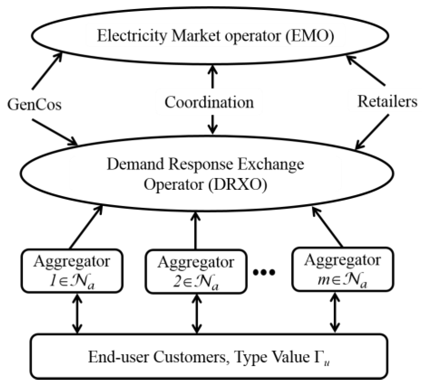
The interactions among several market participants at different levels can be summarised using Figure 1. The upper-level deals a security constraint economic dispatch (SCED) while the lower-level is about the DRX and the aggregators. The division of the market mechanism in DRX can be either horizontal among aggregators or vertical among the end-users and the aggregator. In the proposed DRX mechanism, the users get paid by the aggregator for their DR capable loads. To solve the DRX integrated market clearing model, a bi-level optimization technique has been used [26,40].

The DR supply offer is made available in a separate DRX market at the lower-level. The user’s inconvenience cost is minimized while achieving the targeted DR at the upper-level. The interaction between the aggregators and the users in the DRX market is modelled as a mechanism design problem. The aggregators make a demand reduction bid, and the DRX operator (DRXO) determines the DR share among the aggregators to minimize the DR transaction cost. At the upper-level, the interaction between GenCos and EMO is modelled as a SCED problem, where the generation supply offer bid is settled by the EMO, aiming to minimize operation cost based on the reduced demand and transaction cost at the lower-level.

The bi-level interaction is formulated as a mathematical programming problem with complementarity constraints [41,42,43]. The aggregator’s payoff comprises of the difference of DR selling revenue at the locational marginal price (LMP) and compensation provided to the customers. The LMP and compensation price is obtained by solving the lower and upper-level problem, respectively. A Lagrangian duality with associated Karush Kuhn Tucker (KKT) optimality conditions is used to solve the bi-level optimization. A gradient descent algorithm is also identified to solve bi-level electricity market model as reported in [44]. The effectiveness of the proposed market model is demonstrated on a PJM 5-Bus benchmark power system considering several case studies. The proposed DR integrated market model minimizes the operation cost, and maximizes the aggregator’s payoff within a certain incremental DR level.

Let us consider a set, $\mathbb{T}$:= {0, …, T_k − 1}, is a time period, and assume that the number of time interval T_k satisfies T_k = 24/k (k = 1 h duration interval). Therefore, the set, $\mathbb{T}$, has 24 components. The proposed market model can be framed as a bi-level programming problem given by Equations (1)–(16). Equations (1)–(10) and (11)–(16), respectively, represent the upper-level and lower-level problems.

$$\underset{{\mathsf{\Psi }}_{nk}(P_g,P_w)}{\mathrm{Minimize}}{\displaystyle \sum _{\forall n\in {\mathcal{N}}_{ℊ}}{c}_n(P_{g_{nk}})P_{g_{nk}}}+{\displaystyle \sum _{\forall m\in {\mathcal{N}}_{𝓇}}{\lambda }_{mk}^d}{d}_{mk}$$

(1)

Subject to:

$${\displaystyle \sum _{\forall n\in {\mathcal{N}}_{ℊ}}{P}_{g_{nk}}}={\displaystyle \sum _{\forall i\in {\mathcal{N}}_{𝒷}}(1-{\chi }_w)D_{ik}}+{\displaystyle \sum _{\forall (i,j)\in {\mathcal{N}}_{𝓁}}{\mathrm{B}}_{\mathrm{b}}({\vartheta }_{ik}-{\vartheta }_{jk})}\leftrightarrow {\lambda }_{ik}^S$$

(2)

$${\mathrm{B}}_f({\vartheta }_{ik}-{\vartheta }_{jk})\le F_{ij}\forall (i,j)\in {\mathcal{N}}_{𝓁},\forall k$$

(3)

$$F_{ij}^{\min }\le F_{ij}\le F_{ij}^{\max }\leftrightarrow {\nu }_{lk}^F\forall (i,j)\in {\mathcal{N}}_{𝒷}$$

(4)

$$P_{g_{nk}}^{\min }\le P_{g_{nk}}\le P_{g_{nk}}^{\max },\leftrightarrow \{{\lambda }_{g,k}^{\mathrm{S},\min },{\lambda }_{g,k}^{\mathrm{S},\max }\}\forall n\in {\mathcal{N}}_{ℊ},\forall k$$

(5)

$$R_n^{dn}\le P_{g_{nk}}-P_{g_{nk-1}}\le R_n^{up},\forall k,\forall n\in {\mathcal{N}}_{ℊ},\forall k$$

(6)

$${\vartheta }_i^{\min }\le \vartheta \le {\vartheta }_i^{\max },\forall i$$

(7)

$${\vartheta }_{i=1}^{}=0\mathrm{when}i\mathrm{is}\mathrm{the}\mathrm{slack}\mathrm{bus}$$

(8)

$$0<D_{ik},{\chi }_w\in \mathbf{R},\forall k,\forall i\in {\mathcal{N}}_{𝒷}$$

(9)

$$\mathrm{where}0<{\lambda }_{mk}^d,0<d_{mk}\in \arg \mathbf{Minimize}\{$$

(10)

$$\mathrm{DRTC}={\displaystyle \sum _{\forall m\left|\right(m,j)\in {\mathcal{N}}_{𝒶}}{s}_{m,u}(d_{mj}^k})d_{mj}^k$$

(11)

Subject to:

$${\displaystyle \sum _{\forall m\left|\right(m,j)\in {\mathcal{N}}_{𝒶}}{\mathrm{A}}_a{\mathit{d}}_{mj}^k}={\displaystyle \sum _{\forall j\left|\right(m,j)\in {\mathcal{N}}_{𝓇}}{\mathrm{A}}_r{\mathit{d}}_{jm}^k},\leftrightarrow {\lambda }_{mk}^d\forall m,\forall j$$

(12)

$${\displaystyle \sum _{\forall j\in {\mathcal{N}}_{𝓇}}{\mathrm{A}}_r{\mathit{d}}_{jm}^k}={\chi }_w{D}_{ik},\leftrightarrow {\lambda }_{j,k}^d,\forall m,\forall k,\in {\mathcal{N}}_{𝒷}$$

(13)

$$r_{mj}^{\min }\le d_{mj}^k\le r_{mj}^{\max },\leftrightarrow \{{\lambda }_{mj,k}^{d,\min },{\lambda }_{mj,k}^{d,\max }\text{}},\forall k,\left(mj\right)\in \mathcal{A}$$

(14)

$$|d_{mj}^k-d_{mj}^{k-1}|\le \mathsf{\Delta }{d}_{mj}^k,\forall k,\left(mj\right)\in \mathcal{A}$$

(15)

$$0\le d_m^k\le d_m^{\max },\forall k,\forall m\in {\mathcal{N}}_{𝓊}.\}$$

(16)

2.1. SCED’s Problem at Upper-Level

A power system network represents an optimal power flow (OPF) model with a number of N_b buses, and N_l transmission lines are considered [25]. In the model, $𝒩$_𝒷 is the set of busses and $𝒩$_𝓁 the sets of the transmission lines, respectively. Further, define $𝒩$_ℊ:= {1, 2,…, N_g} is the set for the generation companies. The demand at the ith bus is denoted by D_i,∀i ∈ $𝒩$_𝒷. The operation cost in (1) consists of two terms. The first term, c_n$(P{g}_{nk}^{}$), refers to the offers cost of the generation $P{g}_{nk}^{}$ units. The second term, ${\lambda }_{mk}^d,$ refers to the demand reduction cost for the $d_{mk}^{}$ is for the DR amount provided by aggregator m in time k. The equality constraint (2) represents the grid wise supply-demand balance. The first term on the right-hand side of this constraint is a DR regulating factor. The B_b is for the bus admittance matrix. The term, (ϑ_ik − ϑ_jk), is for the voltage phase angles. Representing x_ij for the reactance of the transmission line from the bus i and j, the diagonal element of the B_b is the sum of all 1/x_ij. The off-diagonal element of the B_b is equal to the negative of 1/x_ij, between the bus i and j. The power flow in the lines connecting the bus i and j are represented by Equation (3). The details refer to [25,45,46]. The transmission line and generation supply limits are provided in Equations (4)–(6), respectively. The associated dual variables contracting to the constraints are presented by the double-headed arrow. The ramping rate constraints are given in Equation (6). The constraint Equation (7) imposes voltage phase angle limits. The nonzero decision variables in Equation (10) are found by solving the lower-level DRX optimization model.

The few key assumptions in this model are that the offer pricing scheme in the market clearing model does not consider any source of non-convexities, such as start-up costs of the generating plants or their up/downtime constraints, for simplicity reasons. Also, a direct current approximation of the power system is used where the voltage magnitude in buses of the network is assumed to be unity, the voltage phase differences small, and the transmission lines are lossless, and no security criterion, like outage of transmission lines or generators, is considered.

2.2. DRX’s Problem at Lower-Level

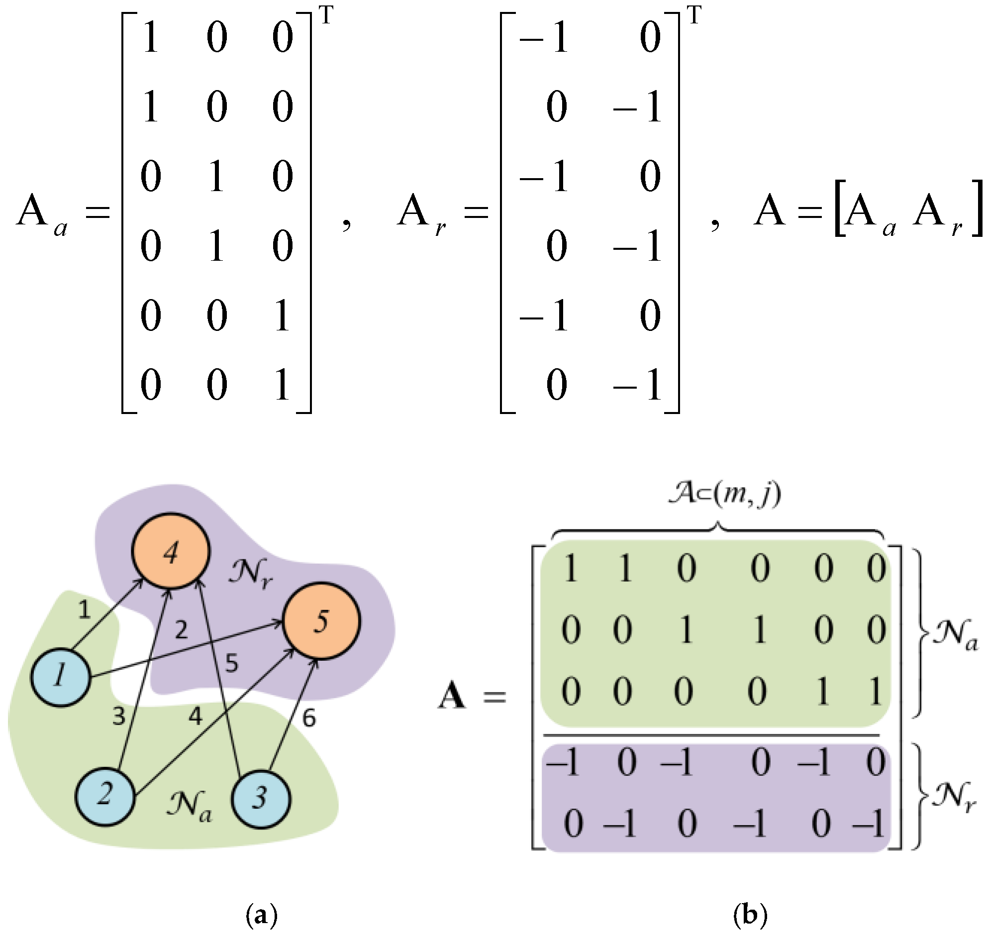
The lower-level problem fixes the optimal DR amount to be traded and the DR transaction cost. The DRX market can be constructed as a directed graph, $ℒ$: = ($𝒩$, 𝒜), indicated by the node set, $𝒩$, composed with an arc set, 𝒜 ⊂ (m, j), joining the trading node m and j as presented in [25]. Two different nodes in L, namely $𝒩$_𝒶: = {1, 2, …, N_a} and $𝒩$_𝓇: = {1, 2, …, N_r}, corresponding for the DR aggregator and DR purchaser (as see Figure 2). The DR buyers are simplified as those price-sensitive load buses where the unit load reduction save more operation cost.

The dealings between buyers and aggregators in $ℒ$ are denoted using the node-arc incidence matrix, A, organized of the vertical concatenation of matrix A_a and A_r. For three aggregators (N_a = 3) and two buyers, (N_r = 2), the matrices, A_a and A_r, in Equation (14), take the arrangement as shown in Figure 2.

The quantity of rows in A_a and A_r is equal to the number of aggregators and buyers, respectively. It is assumed the aggregator can sell the DR to several buyers, and each of the DR buyers can buy the DR from several aggregators. The total number of possible deals between the DR buyer and aggregators denote the number of columns of the A matrix. Any DR quantity, d_mj (d_mj > 0), associated with arc, (m, j) ∈ A, represent the DR transaction from the aggregator node, m ∈ $𝒩$_𝒶, to the DR buyer node, j ∈ $𝒩$_𝓇. The objective function (13) specifies the DR resource cost function (s_m,,u) of the end-user customer, u, under the aggregator, m. The bidding price rises with the growing level DR as represented by:

$$s_{m,u}={\omega }_m({\alpha }_m{d}_{mj}^2+{\beta }_m(1-{\mathsf{\Gamma }}_u)d_{mj})$$

(17)

The term, ω_m, is the aggregator’s bidding factor, which is used to characterize aggregator price-taking behaviour [26]. The lower the ω_m value; the lesser is the price escalation and vice versa. The ω_m value can be determined by tracking the LMPs and end-user’s consumption flexibility [47]. The quadratic (α_m) and linear (β_m) coefficient terms are assumed to be unity. The Γ_u, ∀i is called end-user type, which takes values between 0 and 1. The non-negativity of type value scales user wiliness to adjust compensation price [48,49,50]. At a higher value of Γ_u, users are likely to waive compensation for the equal quantity of DR. This intern reduces the DR transaction cost.

For a set of optimal decision variable, d_mj (also called primal variable), of length, N_a × N_r, the objective function (11) returns a scalar DR transaction cost. The constraint (10) specifies the sum of DR from all aggregators is equal to the total DR provided to DR buses. The coupling constraint (12) refers to the summation of the DR from all the DR buses is as large as the DR limits imposed by the operator.

The term, χ_w (χ_w ∈ R), introduced in the upper-level is a regulation parameter for the DR level settings, which limits load demand, D_i, at a power system bus, i, i ∈ $𝒩$_𝒷. Based on the exogenous variables, such as the adjustment required for the renewables, the total DR from the reference consumption is to be increased or decreased.

The aggregator’s DR collecting behaviour, which can be regulated by the DRXO, may increase the number of end-users by providing a higher compensation rate. The constraint (13) set by the DRXO relates the minimum and maximum DR limits over any transaction, (m, j) ∈ 𝒜. The constraint (14) limits the pick-up/drop-off rate. The constraint (18) specifies that the DR from an aggregator does not exceed its maximum capacity limits, $d_m^{max}$.

Assume a vector of dispatch decisions at k^th step Ψ_nk: = [Pg_1k, Pg_2k, …, Pg_Ngk]’ to represent the generation profile. Define further dispatch decisions considering the DR are Ψ_nk^DR: = [Pg_1k^DR, Pg_2k^DR, …, Pg_Ngk^DR]’ accordingly. Where the Ψ_nk to Ψ_nk^DR, respectively, denote generation without and with DR, respectively. The aggregator’s profit (0 < R_m, ∀m) is the difference of a percentage of total cost saving due to the DR and the compensation given to the end-user customers.

$$R_m={\gamma }_m{\displaystyle \sum _{\forall (n,k)}\left\{{\lambda }_{nk}^S\left({\mathsf{\Psi }}_{nk}\right){\mathsf{\Psi }}_{nk}-{\lambda }_{nk}^S\left({\mathsf{\Psi }}_{nk}^{\mathrm{DR}}\right){\mathsf{\Psi }}_{nk}^{\mathrm{DR}}\right\}}-{\displaystyle \sum _{\forall (m,k)}{s}_m(d_{mk}^k})$$

(18)

where the λ^S_nk(Ψ_nk) and λ^S_nk(Ψ_nk^DR) are the LMP without and with the DR, respectively. The term in the bracket in Equation (18) corresponds to the total LMP reduction. The term, α_m, is for a percentage of monetary reward; aggregator obtains from the operator. The term, γ_m, equals to unity reflect the aggregator gets paid at a rate of the LMP. The γ_m > 1 means the payment is made at a rate that is higher than the LMP. This indirectly subsidizes the end-user to increase the incremental curtailment. The γ_m < 1 refers a partial amount of the LMP is given to limit the DR trading.

Note that the DR bid influences the LMP and consequently reduces the electricity operation cost. For a given value of DR, the actual reduction in the operation cost and the LMP may be different depending on the strategic supply bidding game of the GenCos. The aggregator’s payoff would be cost-effective when the end-user’s DR payment cost is lesser and the LMP is greater.

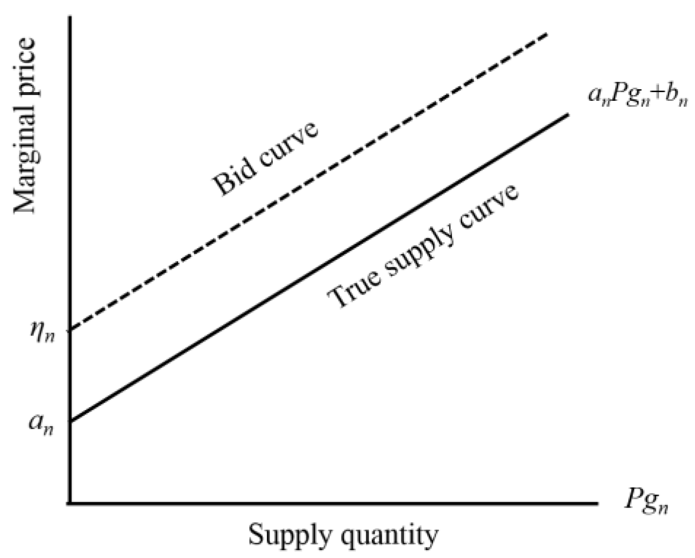
The GenCo has its own supply cost ($) curve, usually in quadratic form. Indeed, GenCo submits an hourly supply offer at the marginal price ($/MWh). The marginal price is of the form, a_nPg_n + b_n, where Pg_n is the generation output of unit n, and a_n, b_n are the cost coefficients. It is customary to submit generation blocks, q > 0, ∀q ∈{1, 2, 3, …, Q}; the seller wants to sell at a price, constitute stepwise price-generation block pair expressed by:

$$c_n(P_{g_{nq}})=\{\begin{array}{c}{a}_{n1}(P{g}_n-P_{g_{n1}})+b_{n1},\\ \begin{array}{l}{a}_{nq-1}(P_{g_n}-P_{g_{nq-1}})+\\ \begin{array}{cc}& ⋮\end{array}\end{array}\\ a_{nk}(P_{g_n}-P_{g_{nq}})+b_{nq},\end{array}\begin{array}{c}{P}_{g_n}\le P_{g_{n1}}\\ \begin{array}{l}{b}_{nq-1},P_{g_{n1}}<P_{g_n}\le P_{g_{nq-1}}\\ \begin{array}{cc}& ⋮\end{array}\end{array}\\ P_{g_{nq}}<P_{g_{nQ}}.\end{array}$$

(19)

The number of blocks and its size rely on the generation capacities. In this study, the quantity index, q, is later on replaced by k to calculate a varying generation profile at k^th time step.

Table 1. Generation capacity limits, emission rate, lines, and load data.

Gen (Fuel type)		Capacity Limits[Pnmin Pnmax ] (p.u.)		Carbon Emissions (kgCO2/kWh) [54]
G1 (Coal), Bus#1		[0.25, 1.10]		0.940
G2 (Diesel), Bus#1		[0.25, 1.00]		0.778
G3 (Coal), Bus#3		[1.50, 5.20]		0.940
G4 (Gas), Bus#4		[0.50, 3.00]		0.581
G5 (Coal), Bus#5		[2.25, 6.00]		0.940
Transmission Lines and Load Data
From Bus i	To Bus j	Reactance (xij)	Capacity Limit [Fijmin Fijmax]		Load Demand Di (p.u.)
1	2	2.81	[−8.75, 8.75]		Bus#2 = 3.00
2	3	1.08	[−8.75, 8.75]		Bus#3 = 3.00
4	3	2.97	[−8.75, 8.75]		Bus#4 = 3.00
5	4	2.97	[−8.75, 2.40]
5	1	0.64	[−8.75, 8.75]
1	4	3.04	[−8.75, 8.75]

shows the cost coefficients and the generation limit values [26].

In a competitive market environment; the GenCos are a price taker. Hence, during the auction, the supply offer price is made beyond the true marginal cost. The variation of selling offer around the marginal cost is modelled by incorporating a bidding parameter (α_n) as shown in Figure 3. The GenCo manipulate α_n to increase its revenue when the system load level changes from one critical load level to another.

The solution process of the proposed bi-level model consists of three steps, which are as follows: (Step 1) Implement a Lagrangian duality theorem [51] to convert the lower-level problem by replacing its KKT optimality conditions; (Step 2) consider the decision vector of the lower-level problem as an input parameter for the upper-level problem; and (Step 3) transform the overall problem as a mathematical problem with equilibrium constraints with the technique provided in [52].

3. System Model

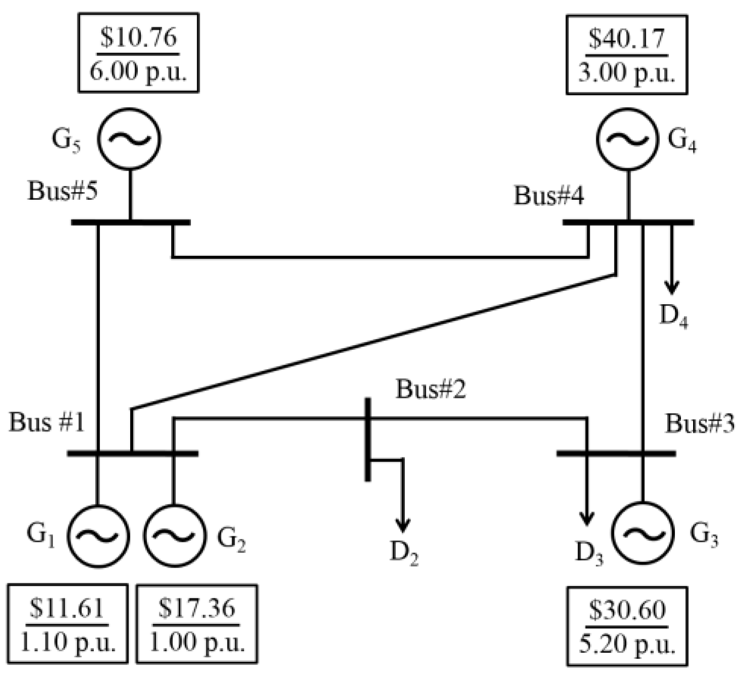
The performance of the proposed market model is investigated on a PJM 5-Bus test power system (Figure 4) consisting of three low-cost (G₁ and G₂ at Bus#1, G₅ at Bus#5); two high-cost generation units (G₃ at Bus#3, G₄ at Bus#4); and the aggregated loads (D₂, D₃, and D_4, at Bus#2, #3, and #4 respectively). The PJM is a regional electric power trading pool market that dispatches the generation and coordinates’ day-ahead capacity and real-time balancing market. It determines the LMP and the generation supply share considering bid-based pricing in a competitive manner. The LMP represents the value of the electricity at the specific location. In the day-ahead capacity market, hourly LMP is determined based on forecasted loads for each hour of the following day. The over or under-estimated loads are adjusted in the real-time balancing market. The test system data, such as generation limits [53] and transmission line parameters [47], are listed in Table 1. The offer prices for all the possible capacities are given in

Table 2. The cost coefficient, bidding quantities, and prices for generation units.

Gen	Block	Generation Supply Offer Price
[an, bn]	Size	[1st Block]	[2nd Block]	[3rd Block]	[4th Block]	[5th Block]
($/MWh, $/MWh2)	(MWh)
G1 [0.115, 11.50]	50.00	11.61, 0.5	17.36, 1.1	23.11	28.86	34.61
G2 [0.115, 11.50]	50.00	11.61, 0.5	17.36, 1.0	23.11	28.86	34.61
G3 [0.355, 12.50]	100.0	12.85, 1.0	30.60, 2.0	48.35, 3.0	66.10, 4.0	83.85, 5.0
G4 [0.425, 18.50]	60.00	18.92, 0.6	40.17, 1.2	61.42, 1.8	82.67, 2.4	103.92, 3.0
G5 [0.265, 10.50]	120.0	10.76, 1.2	24.01, 2.4	37.26,3.6	50.51, 4.8	63.76, 6.0

. The colored numbers in 7^th coloumn are the marginal cost (strategic pursuit to achieve higher profit) to the G₁ and G₄ to deliver an additional unit of electricity at a specific location of the system. The line data, generation capacity, and load demand are at a base of 100 MVA. The upper bound of each aggregator and the DR bidding price for the users under each aggregator are provided in

Table 3. The DR capacity, cost coefficient, and bidding prices.

Aggregator	Capacity	DR Cost Coefficients		The DR Offer Price Segments for the User Group at ωm = 1
	dmax	αm	βm	U1	U2	U3
A1	1.90	0485	12.15	16.97	23.06	27.42
A2	1.70	0.092	10.35	21.71	24.72	26.43
A3	1.70	0.068	11.05	19.20	24.65	24.66
The bidding parameter, ωm in Equation (18), is varied from 1:5.50 with a different increment to rescaled price coefficient, αm and βm, for the different DR levels.

. The EMO collects the supply offer bid and the load demand data. Further, it settles the generation supply share and the LMP. The LMP also was known as the marginal cost to the EMO to deliver an additional unit of electricity at a specific location of a power system. The LMPs ($/MWh) are Lagrangian multipliers determined at the upper-level. The solution of the model assigns the required system load demand among the generation units in such a way that minimized the operation cost.

4. Numerical Result

In this section, three cases are formulated to validate the efficacy of the proposed market model.

Case#1 discusses the congestion-free and congested conditions and the identification of the critical load buses.

Case#2 discusses the competitive bidding (offering bids at a true marginal price) by GenCos and its impact on LMP and the aggregator’s payoff.

Case#3 discusses the strategic bidding (includes a rebidding at higher price and generation capacity withholding when the system load demands exceed crucial load levels) and its impact at the lower-level market clearing.

To enable the DR market mechanism, the critical load buses need to be identified. The critical load buses reflect those buses where a unit load reduction comparatively saves higher operating cost than the rest of the buses. At this end, a cost sensitivity is investigated for different loading levels. The effect of transmission capacity constraints on locational marginal price (LMP) is analyzed.

4.1. Case#1 (Sensitivity Analysis)

The transmission lines in a power system are planned to operate at safe margins with respect to their capacity limit; congestion only happens at some critical lines and are usually well identified. In the congestion-free condition, the transmission lines are not capacity constrained, i.e., they can transfer any amount of power between the buses, and the given demand is met with no locational variation in LMP. For the given test system, the LMP without transmission line constraints is $30.17/MWh, to serve a 3.00 p.u. of the load at Bus#2, Bus#3, and Bus#4 with a total operating cost of k$12.22. The generator, G₁, G₂, G₃, and G₅, provide 1.10, 1.00, 0.90, and 6.00 p.u., respectively. The expensive unit, G₄, does not get dispatched in this instance. Non-zero Lagrange multipliers of value $16.58/MWh and $10.83/MWh are found at the Bus#1 and the Bus#5 as generators G₁, G₂, and G₅ hit their upper limits, respectively. The results are summarized in

Table 4. The generator output and the LMPs to serve load {D₂, D₃, D₄} = {3.00, 3.00, 3.00} p.u.

Scenarios	{G1, G2, G3, G4, G5}	LMPBus # i {λi} ($/MWh)	Total Cost (k$)
Without Line Constraints	{1.10, 1.00, 0.90, 0.00, 6.00}	{30.17, 30.17, 30.17, 30.17, 30.17}	12.22
Line 5–4 is Constrained	{1.10, 1.00, 4.06, 0.00, 2.84}	{28.19, 28.86, 30.60, 31.23, 10.60}	18.48
ΔD2 = ±0.01 p.u.	{1.10, 1.00, 4.05 ± 0.01, 0.00, 2.84}		±$28.86
ΔD3 = ±0.01 p.u.	{1.10, 1.00, 4.05 ± 0.01, 0.00, 2.84}		±$30.60
ΔD4 = ±0.01 p.u.	{1.10, 1.00, 4.05 ± 0.01, 0.00, 2.84}		±$31.23

.

In the congested condition, when line 5–4 is capacity constrained and the maximum power transfer capacity is limited to 2.4 p.u., the market is cleared with high LMP as the cheaper generation cannot be delivered due to the transmission constraint. The LMPs at those five buses are determined to be $28.19/MWh, $32.86/MWh, $30.60/MWh, $31.23/MWh, and $10.60/MWh, as shown in Table 4. The G₃ increases from 0.90 to 4.06 p.u., while the G₅ reduces from 6.00 to 2.84 p.u. The non-zero Lagrangian multipliers due to hitting the upper limits of G₅ are now zero as they are within their limits. The upper limit multipliers for the G₁ and G₂ still exist. The transmission line constraint allowed the G₃ to increase its output and does not hit its upper limit anymore.

The load bus Bus#4 is found to be most sensitive, the Bus#3 is medium, and the Bus#2 is less sensitive. The aggregators are assumed to supply the DR to the most sensitive, Bus#4 and Bus#3. The aggregators bid into the DRX for the incremental DR level to mitigate the LMP spikes. Each of the aggregators has three type/group of users having a different disutility price. The user’s type value defined in aggregator’s DR offer cost function in Equation (18). The DR offer prices are different between two user’s groups. The DR bidding prices are given in Table 3. The offer price continues to rise from the order of low price to high price. However, the bidding parameters are assumed to be constant for a specific DR level.

The DR bidding outcomes determine the transaction cost and compensation price, which can be considered as payback price for the end-users. The load curtailment amount in the DRX market is regulated by the LMP determined in the upper-level market. The aggregators get paid at the LMP rate of those buses where they provide the DR. The aggregator net payoff comprises of the difference of the LMP rate they get paid and the compensation cost provided to the end-users. The DRX market is considered during the peak demand hours, from 6 am to 9 am in the morning and from 4 pm to 8 pm in the evening.

4.2. Case#2 (Competitive Bidding)

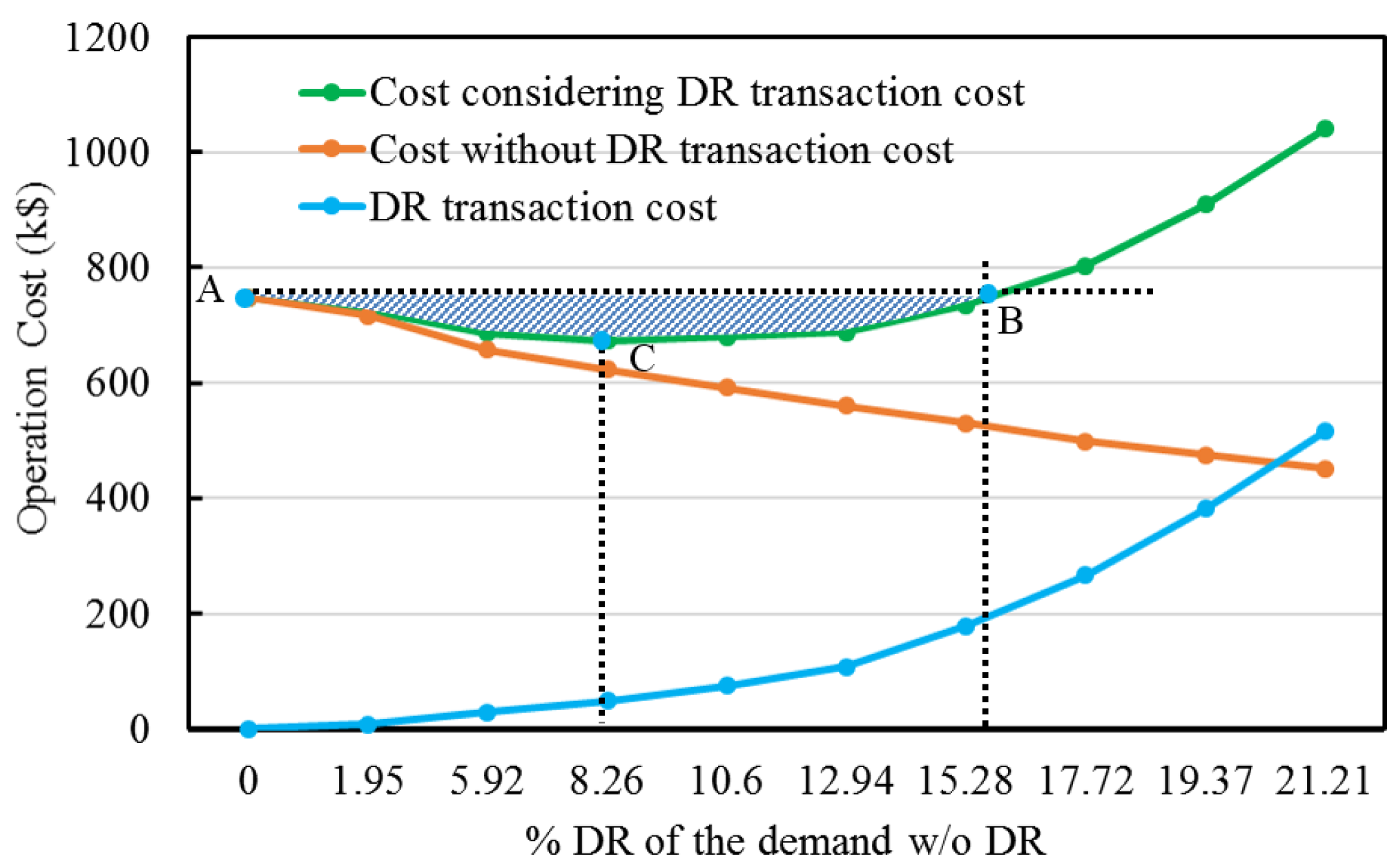
Operation Cost and LMPs: The market model is simulated twice, without and with a DRX mechanism, to quantify the benefits of reduced LMP and operating cost. The operation cost without a DRX is determined to be k$747.49 and an average (over a day) LMP at Bus#4 is found to be $56.49/MWh. The reduction of the LMP ($49.14/MWh LMP at Bus#4) and the operation cost (k$724.16) is evident even with a modest amount of incremental DR (1.95%) for few hours. The effect of different levels of DR on the operating cost with, without DRX transaction cost, is summarized in

Table 5. Operation cost, DRX cost, emission for different DR amount.

DR (p.u.)	Base Demand (p.u.)	DR (%)	Operation Cost with DRX (k$)	Operation Cost w/o DRX (k$)	DR Transaction Cost (k$)	Net Emissions (tonCO2)
0	202.26	0	747.49	747.49	0	19077
4.02	198.18	1.95	724.16	716.41	7.75	18806
12.21	194.08	5.92	686.31	656.96	29.34	18167
17.03	189.25	8.26	672.61	623.84	48.76	17764
21.86	184.42	10.60	679.22	591.78	74.32	17335
26.69	179.59	12.94	687.10	560.78	107.28	16881
31.52	174.76	15.28	734.44	529.78	178.48	16427
36.35	169.94	17.72	802.55	498.79	266.92	15974
39.96	166.32	19.37	909.64	475.36	382.34	15634
43.57	162.71	21.21	1040.62	451.93	516.08	15294

and Figure 5. The operation cost without considering DRX gradually decreases due to serving a reduced load demand. It is interesting to note that with DRX, the operation cost reduces with the DR up to 15.28% and increases for any further increase in DR levels. This is because, at higher DR levels, the DR transaction cost outweighs savings from the reduction in the market clearing cost (the DR transaction cost and the DR amount among the aggregators and users are the decision variables determined by solving the market at the lower-level). The DR transaction cost is reasonably small for up to 12.94% DR and increases sharply beyond it. The DR transaction cost progressively increases with the increasing level of DR. A larger value of DR yields a higher selling revenue for the DRX participants. The DR transaction cost at the lower-level equivalently provides monetary benefit for the end-user customers. The end-user proportionately shares this based on the disutility price they offered. However, the increased DR transaction cost exceeds the overall operation cost provide an argument for limiting the DR payments to periods when the LMP are likely to exceed a specific threshold. The emission without DRX was 19,077 ton a day. With 1.95% and 5.92% DR, the emission reduced to 18,806 and 18,167 ton, respectively. A 1.42% and 6.88% emission, respectively, reduces in each day.

Table 6. Average LMPs ($/MWh) at different buses for incremental DR.

The DR Amount	Average LMP ($/MWh)
% DR	Bus#1	Bus#2	Bus#3	Bus#4	Bus#5
0	50.51	51.82	55.25	56.49	16.28
1.95	47.92	49.14	52.30	53.46	16.28
5.92	46.30	47.45	50.46	51.55	16.28
8.26	45.76	46.89	49.85	50.92	16.28
10.60	44.14	45.21	48.00	49.01	16.28
12.94	44.14	45.21	48.00	49.01	16.28
15.28	44.14	45.21	48.00	49.01	16.28
17.72	44.14	45.21	48.00	49.01	16.28
19.37	44.14	45.21	48.00	49.01	16.28
21.21	44.14	45.21	48.00	49.01	16.28

presents average LMP at different buses in the test system. It is observed that the LMP at Bus#4 is highest and at Bus#5 is lowest (the lower LMP reflects the existence of low-cost generation units to meet demand). The LMP without DR was found to be maximum at Bus#4, and minimum at Bus#5. The LMP at Bus#3 and #4 without DR were $55.25/MWh, and $56.49/MWh, respectively. At 1.95%DR, it reduces to $52.30/MWh and $53.46/MWh, respectively. With the increased DR, the LMP reduces, however, till a certain level and does not further reduce. The LMP was found minimal when the DR level 10.60%. The LMPs, usually, are the basis for payment to generators, aggregators, and payments by the retailers.

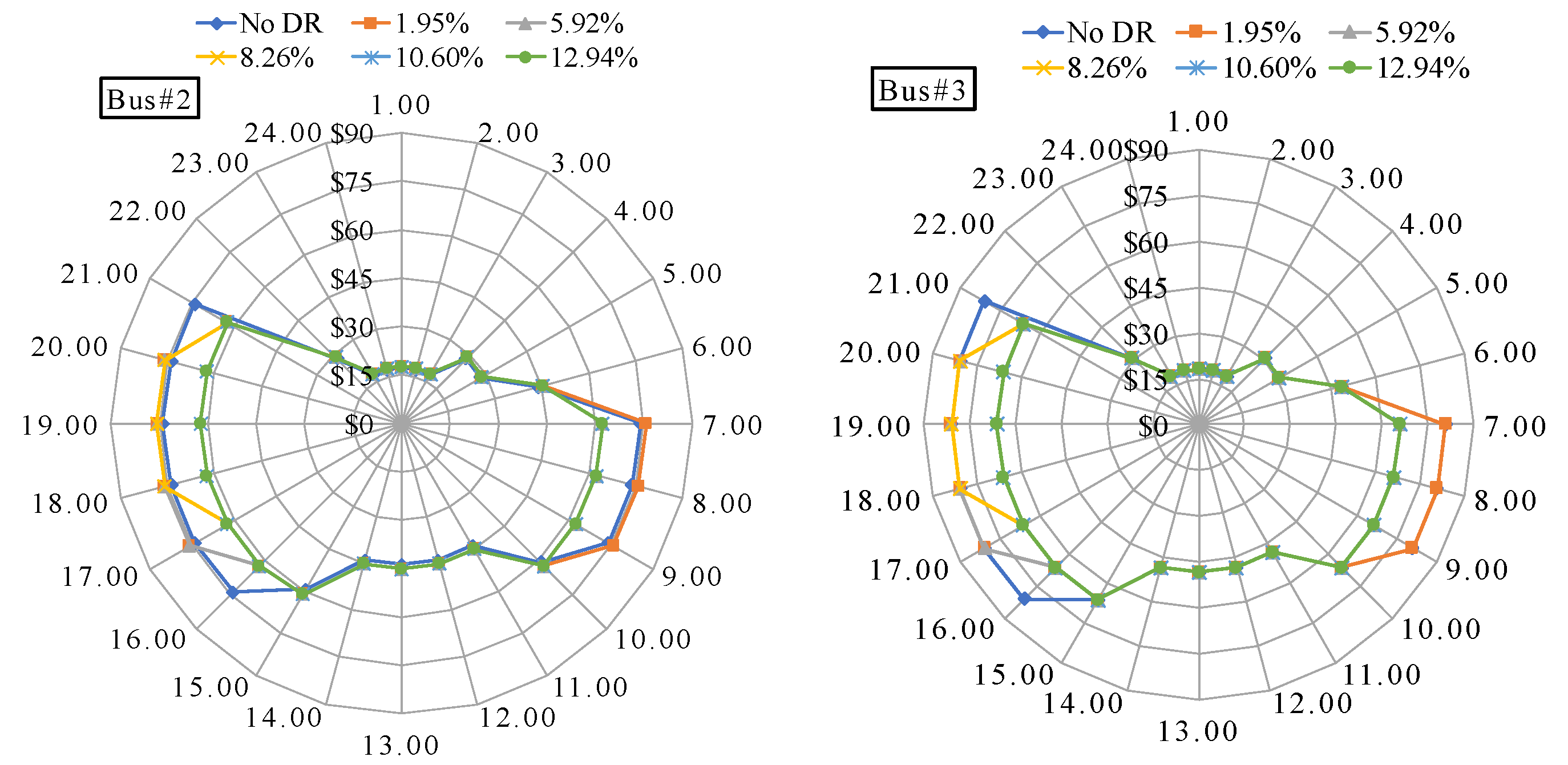
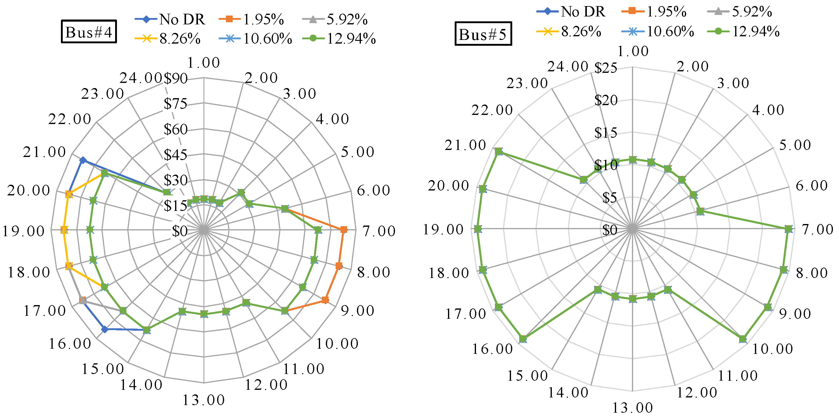
The GenCos and the aggregators are paid at the LMP rate at their respective buses. The radar charts in Figure 6 compare the hourly LMP variation for a day. The radial axis starting from the centre shows the LMP value, while the equiangular distance along the peripheries shows an hour of a day. The hourly LMP is depicted by the marker on the radial axis. The individual line colour represents the LMP with different levels of DR.

The non-peak hour LMP at Bus#2, #3, and #4 does not significantly change. Further, the LMP at the Bus#5 only changes between $10.76 and $24.01. In Bus#5, the unit G₅ get paid as its bid. These values are almost the same irrespective of the DR level. At Bus#2, #3, and #4, the LMPs of the peak demand period are responsive to the incremental DR level. The peak hour LMP at Bus#4, without DR, is found to be $82.67, which reduces to $67.45 at 10.60% DR. At Bus#3, those values are $80.85 and $66.10. At Bus#2, the LMPs are $75.86 and $62.40. Increasing the DR level decreases the peak hour durations. With a DR level of up to 5.92%, the duration of the LMP spike reduces to 4 h in a day and is further reduced to only 3 h for DR level of 8.26% and can be totally avoided with the DR level of 10.60%.

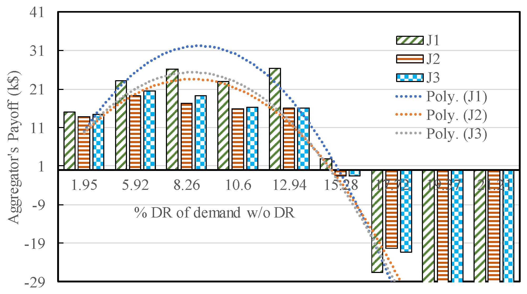
Aggregators’ Payoff: The lower-level model allows the aggregators to participate in the DR exchange in the same way that supply-side Genco’s bid into day-ahead electricity markets. The proposed DRX integrated market clearing model promotes the true market value of DR in daily scheduling intervals. Figure 7 illustrates the aggregators’ payoff with different incremental DR levels and

Table 7. The DR supply share among the aggregators in the DR trading hours in a day.

The DR amount	DR (p.u.) Provided by the Aggregators			The Payoff (k$) Achieved by the Aggregators
% DR	J1	J2	J3	J1	J2	J3
1.95	2.69	2.66	2.66	15.15	13.75	14.41
5.92	4.27	3.97	3.97	23.05	19.35	20.59
8.26	6.70	5.17	5.17	26.09	17.33	19.27
10.60	8.99	6.43	6.44	22.93	15.89	16.19
12.94	11.56	7.57	7.57	26.37	15.98	16.09
15.28	13.98	8.77	8.77	2.92	−1.65	−1.47

presents the DR amount supplied by the aggregators. The aggregator’s payoff not only depends on the amount of DR traded, but also on the LMP. The aggregator payoff is a difference of the DR selling revenue at LMP, and the compensation provided to end-users and is determined using Equation (18). Assuming, the reward scale factor, γ_m, as unity, with a 1.95% DR, the aggregator, A₁, A₂, and A₃, earn k$15.15, k$13.74, and k$14.41, offering the DR amounts of 2.69, 2.66, and 2.66, respectively, in the DR trading period in a day. Irrespective of the equal DR provided by both the J₂ and J₃, the payoff difference happens due to different compensation price among the user group. The payoff rises and becomes maximum at the 8.26% DR level. After a 12.94% DR, a payoff reduction is observed, because of the decrease in the LMP and increase in the rate of compensation price. At the 15.28% DR level, A₁ becomes marginally profitable and both A₂, A₃ outweigh compensation paid to the end-users than the LMP at which the A₂ and A₃ get paid. For any DR levels greater than 17.72%, all the aggregators lose. The polynomial fit (second order) of the payoff is also shown in the figure. As observed, with the increasing DR level, the payoff increases, reaches a maximum value, then decreases before finally becoming zero, at which point, the EMO also loses. Until such a critical DR level, the DR payoff resulting from new revenue generation driven by DRX market is considerable.

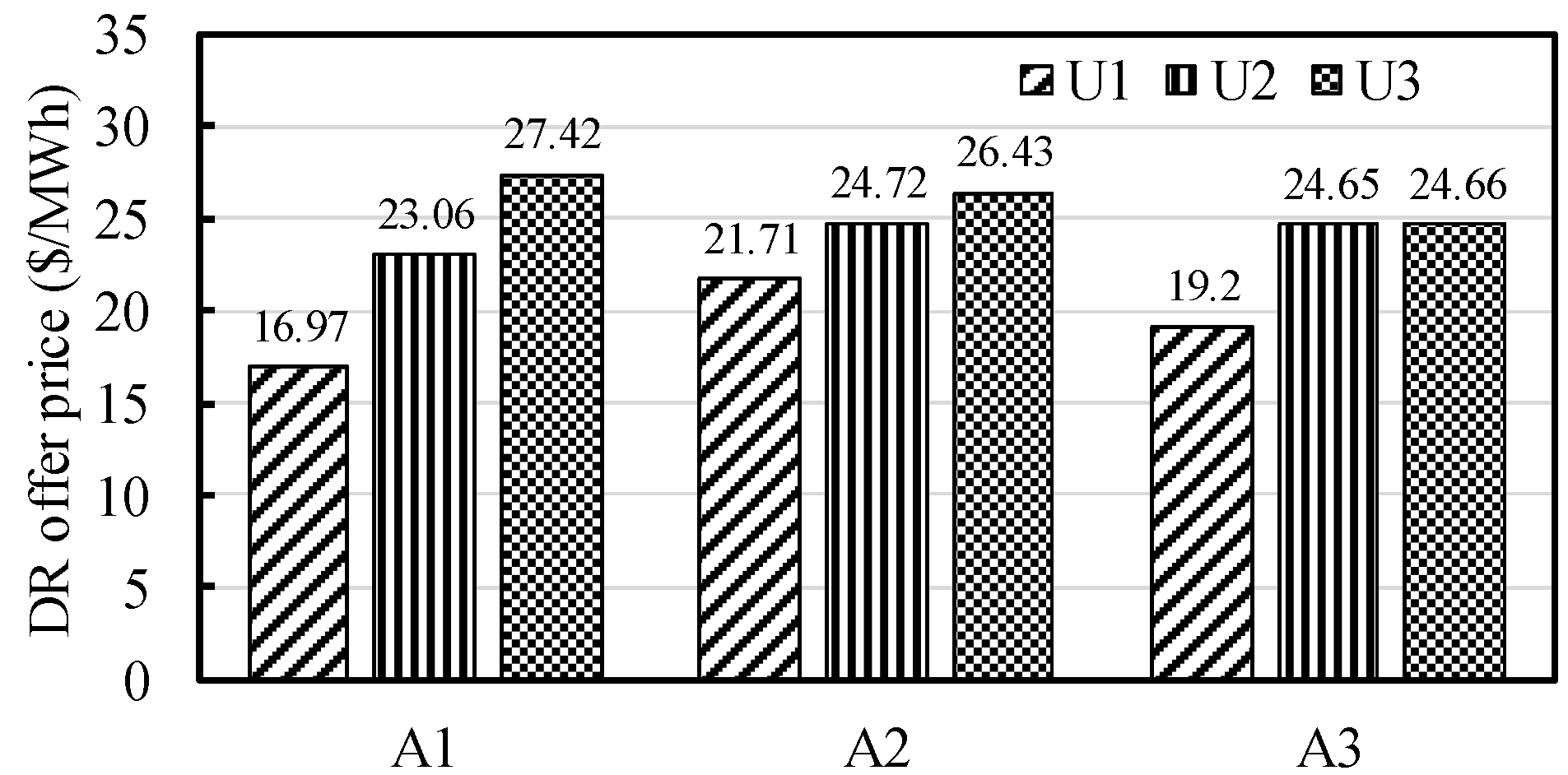
DR and Compensation Share among the End-Users: In the proposed model, aggregators compensate the users for the DR that they provide. The transaction cost and compensation price are determined in DRX markets. The magnitude of possible DR transaction cost depends on how much the users can afford and the marginal disutility price. Figure 8 shows a disutility price for different user groups. Three types/groups of users under each aggregator are considered. The disutility price for user group, U_1, under the aggregator, A₁, is the stepper. The DR price is smallest for the U₁, while it is highest for the U₃. The user, U₁, under the A₂ has minimum disutility ($21.71), while a maximum for the group, U₃ ($26.43). The offer price for the U₁ under aggregator, A₃, is $19.2. The price for the rest of the two group, U₂ and U₃, is around $24.60. The aggregator, A₁, has a maximum DR supply capacity of 2 p.u. and A₂ and A₃ whereas having the capacity of 1.75 p.u. The end-users get paid by the aggregator at a compensation price, which is a dual multiplier associated with Equation (12) of the lower-level problem. Due to receiving compensation (payback), the users reduce the energy consumption cost. However, from the EMO perspective, the DR benefit can be obtained if the operation cost reduction at the upper-level does not outweigh the compensation given to the end-users at the lower-level. This possibly occurs when the DR demand rises significantly higher if the user seeks higher compensation. Multiplying the DR price with the allocated DR is regarded as overall DR compensation benefit for the users.

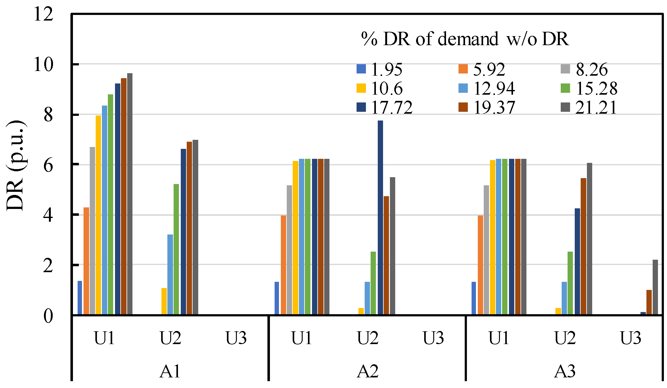
Figure 9 presents the optimal DR amount provided by the user groups for each incremental DR level. The DR transaction cost, the amount supplied, and the compensation price is found by solving the lower-level problem. Until a 10.60% DR, the user group, U₂, under the aggregators do not provide any DR amount. From 10.60 to 15.28% DR; both the U₁ and U₂ deliver with a varying amount. At a 17.62% DR and onward, all the user group under the aggregator, A₃, contribute to supply.

The DR compensation is given in

Table 8. DR compensation provided to end-users with incremental DR.

The DR Amount	Aggregator, A1			Aggregator, A2			Aggregator, A3
% DR	U1 (k$)	U2(k$)	U3(k$)	U1(k$)	U2(k$)	U3(k$)	U1(k$)	U2(k$)	U3 (k$)
1.95	2.31	0	0	2.88	0	0	2.553	0	0
5.92	9.06	0	0	10.76	0	0	9.519	0	0
8.26	17.05	0	0	16.82	0	0	14.88	0	0
10.60	30.14	4.28	0	25.37	1.23	0	23.22	1.22	0
12.94	36.84	14.75	0	30.82	6.59	0	30.73	6.57	0
15.28	52.66	32.97	0	42.37	17.22	0	42.25	17.17	0
17.62	71.33	55.01	0	53.93	32.29	0	53.78	36.46	0.943
19.37	95.62	76.20	0	69.33	52.65	0	69.15	60.34	10.98
21.21	121.28	96.33	0	86.88	76.94	10331	84.54	82.37	30.01

. At the 8.26% DR level, the compensation benefit provided to the user groups are determined to be k$9.06, k$10.76, and k$9.52, respectively. The DR transaction cost at 5.92%DR is $29349. Next, at 8.26% DR, transaction cost increases to $48762. A k$19.41 increase due to 2.34% DR level. The cost increases sharply as the DR requirement rises. At 17.72% DR, the transaction cost increases almost three times than that of the cost at 8.26% DR. The higher transaction cost due to rising DR compensation offer price is neither profitable for the aggregator nor to the EMO. As seen from the DRX integrated operation curve (Figure 5), the DRX integrated market cost gradually decreases with the incremental DR level. The cost reaches a minimum of 8.26% DR. Further, it started to increase, and about 15.28% DR, the DRX integrated operation cost become equal to the cost without DRX. From the economic point of view, the DR integration level should be less than 15.28% DR.

The payoff margin of the aggregators varies with the DR level (Figure 7) and the trend line shows that the maximum payoff is achieved at the 8.26% DR level. The payoff reduces as the DR level rises. At 15.28% DR, the payoff is marginal for the A₁, while for the A₂ and A₃, DR transaction is profitable. Now, if the LMP scaled parameter, γ_m, is increased, then the payoff margin also increases to transact higher amount of DR, provided end-users kept their compensation price fixed.

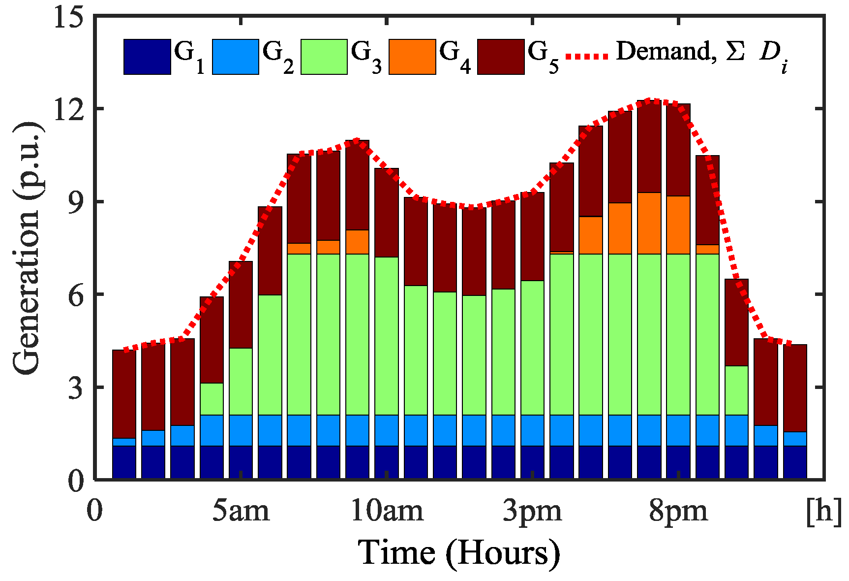
Generation DispatchShare: The solution of the upper-level economic market clearing problem finds the optimal generation dispatch. The G₁, G_2, and G₅ bid a lower price than others. In the market clearing model, the generation units’ output is arranged according to the transmission security and economy-based merit order. Figure 10, Figure 11 and Figure 12 compare the optimal generation dispatch without and with DRX (with two different DR level), respectively. Without DRX, the generation unit, G₁ and G₂, are at their maximum capacity, while the G₃ and G₄ change within its generation limits across the scheduling hour (as in Figure 10). The amount supplied by G₅ is restricted by line capacity constraint, thereby, most of the time, its output changes around 2.85 p.u. The dotted line in red colour indicates the total load demand served by all the generators.

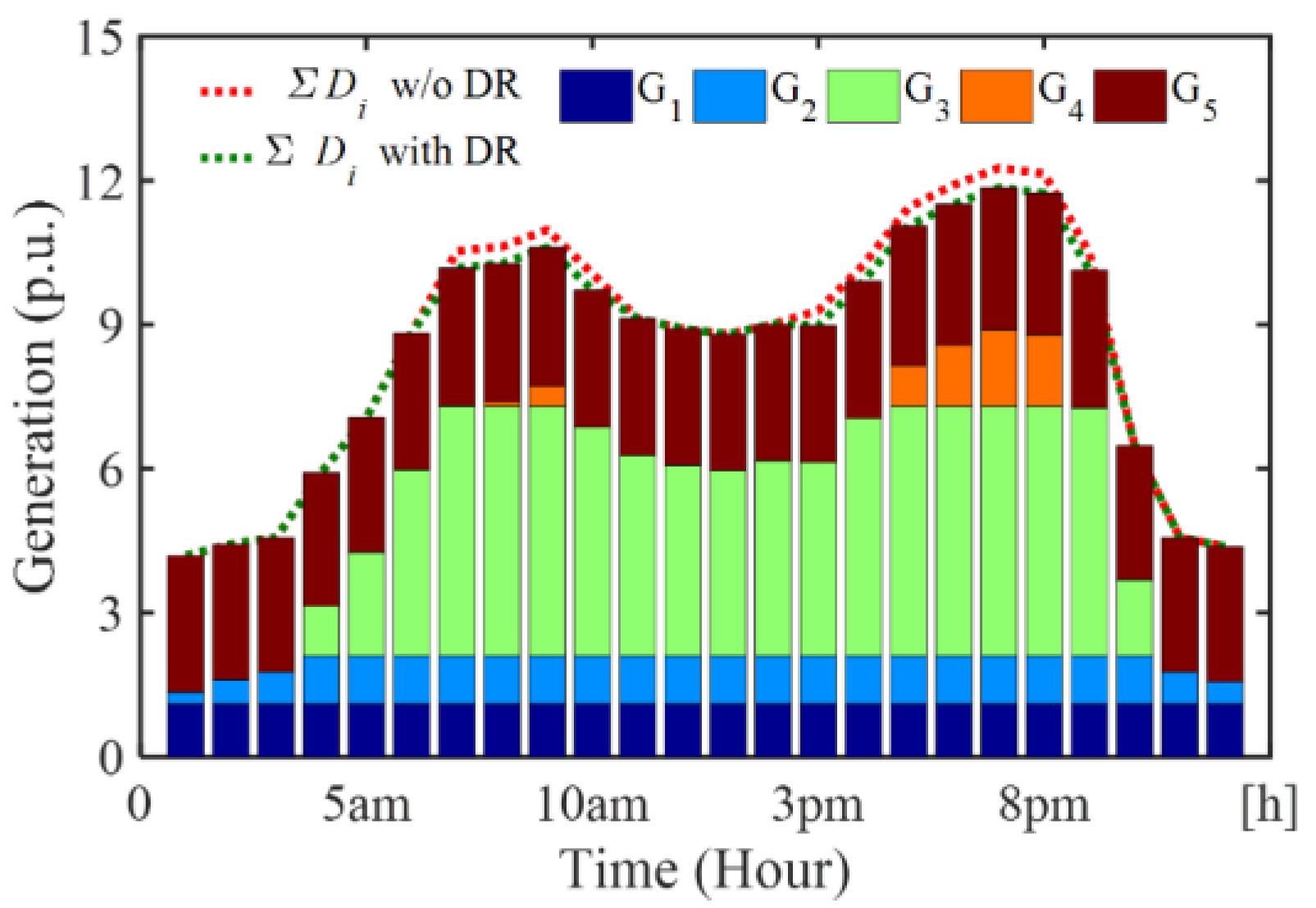
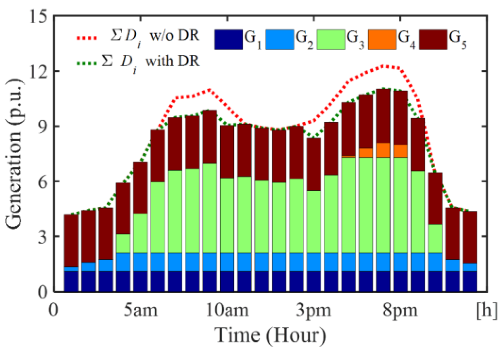
With the proposed DRX model and with a 1.95% DR participation, the total demand without and with DR is shown by the red and green colour in Figure 11. The DR amount, which is the difference between those two curves, becomes higher during the peak period. It is observed that the G₄ is not dispatched at hours 7 am to 9 am as peak loads are curtailed. The G₄ dispatches a few hours around evening peak. Further, in Figure 12, with 5.92% DR, the G₄ only dispatches around evening peak periods. Such dispatch results are economical, since the most expensive unit got restriction. The reduced dispatch of G₄ is compensated mainly by the second least expensive unit, G₃, to meet the load.

4.3. Case#3 (Strategic Bidding)

In strategic bidding, the GenCo bids at a higher price by price distortion or generation capacity withholding deliberately. This is not a routine practice, rather adopt this strategy when the system load demand during the peak hours exceeds significant load levels. It would argue that such opportunistic behaviour cannot always be perceived as profitable [55]. Usually, the GenCos are prone to exercise market power and try to increase their revenue, eventually yielding to a higher overall operating cost [56]. The strategic bidding was mostly attributed to the expensive units. The impact on dispatch share, LMPs, operation cost, and aggregator’ payoff is investigated considering the following scenarios:

Scenario#1: The unit, G₃, bids $83.85 instead of $66.10 in the hour 7 pm, 8 pm, and 9 pm. The unit, G₄, and others bid as completive.

Scenario#2: The unit, G₄, bids $103.92 instead of $82.67 in those hours indicated in Scenario#1. The unit, G₃, and others bid as completive.

Scenario#3: Both the G₃ and G₄ bid simultaneously with the new offer price, while others bid as completive.

Therefore, Scenario#1, Scenario#2, and Scenario#3, respectively, consider strategic bidding of the unit G₃ only, the unit G₄ only, and both the G₃ and G₄ simultaneously. The rest of the conditions, like loading level, transmission constraints, and the capacity of the rest of the units, are the same. The impact on dispatch share, LMPs, and operation cost are investigated.

Table 9. A comparison of aggregator’s payoff for GenCos’ different strategies.

	All GenCos Competitive (Case#2)	The G3 Strategic (Scenario#1)	The G4 Strategic (Scenario#2)	The G3, G4 Both Strategic (Scenario#3)
Aggregator’s Payoff ($) without DR	0	0	0	0
Aggregator’s Payoff (k$) with 5.92% DR	{23.05, 19.35, 20.59}	{23.42,19.70, 20.95,	{21.69, 18.06, 19.31}	{24.72, 20.94, 22.18}
Aggregator’s Payoff (k$) with 8.26% DR	{26.09, 17.32, 19.27}	{23.42, 19.70, 20.94}	{30.16, 20.72, 22.67}	{32.22, 22.43, 24.37}
Total Payoff with 5.92% DR	62.99	64.07	59.07	67.84
Total Payoff with 8.26% DR	62.69	73.86	73.56	79.01
Relative payoff variation with 5.92% DR		(64.07 – 62.69) = 2.20	(59.07 − 62.99) = −6.22	(67.84 − 62.99) = 7.69
Relative payoff variation with 8.26% DR		(73.86 − 62.99) = 17.33	(73.56 − 62.69) = 17.33	(79.01 − 62.69) = 26.03

shows the impact of GenCos strategic bidding on aggregator’s payoff. The payoff set of each aggregator at different DR levels is shown in a second and third row. The sum of the payoff for all aggregators is presented in the fourth and fifth row. At 5.92% DR, the payoff maximum was accounted to be k$67.84 in Scenario#1, while minimum at competitive bidding determines to be k$62.99. A relative payoff variation was determined to be $k2.2. In the same DR level at Scenario#3, the relative increase payoff rises to k$7.69. It is observed that at 8.26% DR, the payoff maximum accounted to be k$79.01 in Scenario#3, while minimum at competitive bidding determines to be k$62.69. A relative payoff variation is $k20.03. As seen, the corresponding payoff for the Scenario#1 and Scenario#2, comparison to the competitive case is almost the same accounted to be k$17.33. In conclusion, GenCos strategic bidding enhances aggregator’s payoff, the payoff is comparatively higher if the number of GenCo practice strategic bidding becomes higher.

The supply offer prices for strategic bidding are highlighted in Table 2.

Table 10. A comparison of operation costs for a different degree of the strategy adopted by GenCos.

	All GenCos Competitive (Case#2)	The G3 Strategic (Scenario#1)	The G4 Strategic (Scenario#2)	The G3, G4 Strategic (Scenario#3)
Operation cost (k$) without DR	747.49	772.07	753.61	764.99
Operation cost (k$) with 5.92% DR	686.31	706.04	687.97	711.65
Operation cost (k$) with 8.26% DR	672.60	690.65	681.31	697.08
Relative increase (%) in cost at 5.92% DR		2.87	0.24	3.69
Relative increase (%) in cost at 8.26% DR		2.68	1.29	3.64
Average LMP ($/MWh) in Bus#4 without DR	54.72	54.98	56.49	56.49
Average LMP ($/MWh) in Bus#4 at 5.92% DR	51.55	51.94	53.32	53.32
Average LMP ($/MWh) in Bus#4 at 8.26% DR	50.92	51.94	52.57	52.57

compares the operation cost and the LMPs for competitive and strategic bidding. The operation costs at 5.92% and 8.26% DR are shown in this table. The second rows show the cost without DR, while the third and fourth are for the 5.92% and 8.26% DR. In Scenario#1, when the G₃ is strategic, the operation cost rises to k$764.99. In Scenario#2 and #3, the cost is k$753.61 and k$772.08, respectively. The relative decrease in operating cost compared to the competitive case found to be maximum at Scenario#3 is 3.69%.

The strategic bidding must clear the market with a higher price. The LMP average over a day in Bus#4 without the DR for the Scenario#1, Scenario#2, and Scenario#3 was found to be $54.98, $56.49, and $56.49, respectively. The DR reduces the price anyway. In Scenario#3, with a 5.92% DR, the average LMP at Bus#4 was found to be $52.57, which was $50.92 in competitive Case#2. At this DR level, the strategic bidding increases the LMP $1.67/MWh.

In summary, the Scenario#3 is the worst-case bidding, which escalates the operating cost to a maximum, keeping the dispatch share the same as that of the competitive case. However, the aggregator’s payoff is higher when a higher number of generators adopt strategic bidding.

5. Conclusions

This paper presents a market framework to effectively integrate DR and reduce wholesale electricity prices. An exemplary DRX market for three aggregators, each having three types of customers, has been modeled. In the model, the aggregators can provide predictable DR services at short notice, which is manageable in real-time. Several plausible bidding behaviors of the market participants have been considered.

Simulation results compare the market clearing price, GenCos’ revenue, aggregator’s payoff, and the amount and cost of the transacted DR. Both competitive and strategic bidding scenarios with different levels of strategies were investigated. The proposed DRX scheme ensures that the least cost operation is achieved either by increasing DR when the GenCos bid strategically or decreasing the amount of DR when the GenCos bid competitively. In competitive bidding, the operation cost is the lowest, which means the DR amount can be reduced, resulting in reduced customer inconvenience. As a price maker, this strategy pushes the market clearing price higher.

The aggregators are price takers when the GenCos exercise strategic bidding. For the same amount of DR, the aggregators get a higher payoff, which would not have been possible under competitive bidding. The DR was found to be profitable as long as its transaction is cost-effective and economical. However, if the GenCos do not return from the price escalation strategy, they must reduce their dispatch share and will likely face a “missing money” problem where the dispatched energy from the GenCos is less and even reduces further.

In conclusion, the DR can be used to exclude GenCos price-lifting behaviour to some extent while maintaining the minimal energy consumption cost for the end-users. Moreover, the reduction in the overall operating cost, carbon emission, and congestion cost were achieved. However, beyond a critical DR level, the DR compensation price becomes higher, outweighing the benefits.

This paper focuses mainly on DR trading at the wholesale level and a detailed distribution market framework could be explored to allow aggregators to trade DR. Collecting DR from the residential customer under different DR programs in the distribution electricity market should be investigated in the future.

References

- Fang, X.; Hu, Q.; Li, F.; Wang, B.; Li, Y. Coupon-Based Demand Response Considering Wind Power Uncertainty: A Strategic Bidding Model for Load Serving Entities. IEEE Trans. Power Syst. 2015, 31, 1025–1037. [Google Scholar] [CrossRef]
- Faruqui, A.; George, S. Quantifying customer response to dynamic pricing. Electr. J. 2005, 18, 53–63. [Google Scholar] [CrossRef]
- Mohammad, N.; Mishra, Y. Transactive Market Clearing Model with Coordinated Integration of Large-Scale Solar PV Farms and Demand Response Capable Loads. In Proceedings of the 2017 Australasian Universities Power Engineering Conference, AUPEC, Melbourne, Australia, 21–23 November 2017; pp. 1–6. [Google Scholar]
- Vardakas, J.S.; Zorba, N.; Verikoukis, C.V. A Survey on Demand Response Programs in Smart Grids: Pricing Methods and Optimization Algorithms. IEEE Commun. Surv. Tutor. 2015, 17, 152–178. [Google Scholar] [CrossRef]
- Deng, R.; Yang, Z.; Chow, M. A Survey on Demand Response in Smart Grids. IEEE Trans. Ind. Inform. 2015, 11, 1–8. [Google Scholar] [CrossRef]
- Albadi, M.H.; El-Saadany, E.F. A summary of demand response in electricity markets. Electr. Power Syst. Res. 2008, 78, 1989–1996. [Google Scholar] [CrossRef]
- Dave, S.; Sooriyabandara, M.; Zhang, L. Application of a game-theoretic energy management algorithm in a hybrid predictive-adaptive scenario. In Proceedings of the 2nd IEEE PES International Conference and Exhibition on Innovative Smart Grid Technologies (ISGT Europe), Manchester, UK, 5–7 December 2011. [Google Scholar] [CrossRef]
- Märkle-Huß, J.; Feuerriegel, S.; Neumann, D. Large-scale demand response and its implications for spot prices, load and policies: Insights from the German-Austrian electricity market. Appl. Energy 2018, 210, 1290–1298. [Google Scholar] [CrossRef]
- Kiani, A.; Annaswamy, A. Wholesale energy market in a smart grid: Dynamic modeling and stability. In Proceedings of the 2011 50th IEEE Conference on Decision and Control and European Control Conference, Orlando, FL, USA, 12–15 December 2011; pp. 2202–2207. [Google Scholar]
- Ben, F.; David Burns, J.G.D.K.; Samin, M.P.L.; Peirovi, S. Demand Response and Advanced Metering. Available online: https://www.ferc.gov/legal/staff-reports/2017/DR-AM-Report2017.pdf (accessed on 5 August 2018).
- Asimakopoulou, G.E.; Vlachos, A.G.; Hatziargyriou, N.D. Hierarchical Decision Making for Aggregated Energy Management of Distributed Resources. Power Syst. IEEE Trans. 2015, 30, 3255–3264. [Google Scholar] [CrossRef]
- Khan, A.A.; Razzaq, S.; Khan, A.; Khursheed, F. Owais HEMSs and enabled demand response in electricity market: An overview. Renew. Sustain. Energy Rev. 2015, 42, 773–785. [Google Scholar] [CrossRef]
- Setlhaolo, D.; Xia, X. Optimal scheduling of household appliances with a battery storage system and coordination. Energy Build. 2015, 94, 61–70. [Google Scholar] [CrossRef]
- Zhao, Q.; Shen, Y.; Li, M. Control and Bidding Strategy for Virtual Power Plants with Renewable Generation and Inelastic Demand in Electricity Markets. IEEE Trans. Sustain. Energy 2016, 7, 562–575. [Google Scholar] [CrossRef]
- Paterakis, N.G.; Erdinc, O.; Bakirtzis, A.; Catalao, J.P. Optimal Household Appliances Scheduling under Day-Ahead Pricing and Load-Shaping Demand Response Strategies. IEEE Trans. Ind. Inform. 2015, 11, 1509–1519. [Google Scholar] [CrossRef]
- Shariatzadeh, F.; Mandal, P.; Srivastava, A.K. Demand response for sustainable energy systems: A review, application and implementation strategy. Renew. Sustain. Energy Rev. 2015, 45, 343–350. [Google Scholar] [CrossRef]
- Nunna, K.H.S.V.S.; Doolla, S. Responsive end-user-based demand side management in multimicrogrid environment. IEEE Trans. Ind. Inform. 2014, 10, 1262–1272. [Google Scholar] [CrossRef]
- Cappers, P.; Goldman, C.; Kathan, D. Demand response in U.S. electricity markets: Empirical evidence. Energy 2010, 35, 1526–1535. [Google Scholar] [CrossRef] [Green Version]
- Vivekananthan, C.; Mishra, Y.; Ledwich, G.; Li, F. Demand response for residential appliances via customer reward scheme. IEEE Trans. Smart Grid 2014, 5, 809–820. [Google Scholar] [CrossRef]
- Wang, Q.; Zhang, C.; Ding, Y.; Xydis, G.; Wang, J.; Østergaard, J. Review of real-time electricity markets for integrating Distributed Energy Resources and Demand Response. Appl. Energy 2015, 138, 695–706. [Google Scholar] [CrossRef]
- Parvania, M.; Fotuhi-Firuzabad, M. Integrating load reduction into wholesale energy market with application to wind power integration. IEEE Syst. J. 2012, 6, 35–45. [Google Scholar] [CrossRef]
- Gkatzikis, L.; Koutsopoulos, I.; Salonidis, T. The role of aggregators in smart grid demand response markets. IEEE J. Sel. Areas Commun. 2013, 31, 1247–1257. [Google Scholar] [CrossRef]
- Ali, M.; Alahäivälä, A.; Malik, F.; Humayun, M.; Safdarian, A.; Lehtonen, M. A market-oriented hierarchical framework for residential demand response. Int. J. Electr. Power Energy Syst. 2015, 69, 257–263. [Google Scholar] [CrossRef]
- Valinejad, J.; Barforoshi, T.; Marzband, M.; Pouresmaeil, E.; Godina, R.; Catalão, J.P.S. Investment Incentives in Competitive Electricity Markets. Appl. Sci. 2018, 8, 1978. [Google Scholar] [CrossRef]
- Mohammad, N.; Mishra, Y. Coordination of wind generation and demand response to minimise operation cost in day-ahead electricity markets using bi-level optimisation framework. IET Gener. Transm. Distrib. 2018, 12, 3793–3802. [Google Scholar] [CrossRef]
- Mohammad, N.; Mishra, Y. Competition Driven Bi-Level Supply Offer Strategies in Day Ahead Electricity Market. In Proceedings of the Australasian Universities Power Engineering Conference, Brisbane, Australia, 25–28 September 2016; pp. 1–6. [Google Scholar]
- Mohammad, N.; Mishra, Y. Book Chapter, Demand Side Management and Demand Response for Smart Grid. In Handbook of Smart Grid Communication Systems; Kabalci, K., Ersan, Y., Eds.; Springier Nature: Singapore, 2019; pp. 197–231. ISBN 978-981-13-1768-2. [Google Scholar]
- Xu, Y.; Li, N.; Low, S.H. Demand Response with Capacity Constrained Supply Function Bidding. IEEE Trans. Power Syst. 2015, 31, 1–12. [Google Scholar] [CrossRef]
- Nguyen, D.T.; Nguyen, H.T.; Le, L.B. Dynamic Pricing Design for Demand Response Integration in Power Distribution Networks. IEEE Trans. Power Syst. 2016, 31, 3457–3472. [Google Scholar] [CrossRef]
- Saez-Gallego, J.; Kohansal, M.; Sadeghi-Mobarakeh, A.; Morales, J.M. Optimal Price-Energy Demand Bids for Aggregate Price-Responsive Loads. IEEE Trans. Smart Grid 2017, 9, 5005–5013. [Google Scholar] [CrossRef]
- Nguyen, T.; Negnevitsky, M.; Groot, M. De Pool-based Demand Response Exchange: Concept and modeling. IEEE Trans. Power Syst. 2011, 26, 1677–1685. [Google Scholar] [CrossRef]
- Shafie-Khah, M.; Shoreh, M.H.; Siano, P.; Fitiwi, D.Z.; Godina, R.; Osorio, G.J.; Lujano-Rojas, J.; Catalao, J.P.S. Optimal Demand Response Programs for improving the efficiency of day-ahead electricity markets using a multi attribute decision making approach. In Proceedings of the 2016 IEEE International Energy Conference, ENERGYCON, Leuven, Belgium, 4–8 April 2016. [Google Scholar]
- Ayón, X.; Gruber, J.K.; Hayes, B.P.; Usaola, J.; Prodanović, M. An optimal day-ahead load scheduling approach based on the flexibility of aggregate demands. Appl. Energy 2017, 198, 1–11. [Google Scholar] [CrossRef]
- Nan, S.; Zhou, M.; Li, G. Optimal residential community demand response scheduling in smart grid. Appl. Energy 2018, 210, 1280–1289. [Google Scholar] [CrossRef]
- Ampimah, B.C.; Sun, M.; Han, D.; Wang, X. Optimizing sheddable and shiftable residential electricity consumption by incentivized peak and off-peak credit function approach. Appl. Energy 2018, 210, 1299–1309. [Google Scholar] [CrossRef]
- Shoreh, M.H.; Siano, P.; Shafie-khah, M.; Loia, V.; Catalão, J.P.S. A survey of industrial applications of Demand Response. Electr. Power Syst. Res. 2016, 141, 31–49. [Google Scholar] [CrossRef]
- Zimmerman, R.D.; Murillo-Sanchez, C.E.; Thomas, R.J. Matpower: Steady-State Operations, Planning, and Analysis Tools for Power Systems Research and Education. IEEE Trans. Power Syst. 2011, 26, 12–19. [Google Scholar] [CrossRef]
- Sood, Y.R.; Padhy, N.P.; Gupta, H.O. Deregulated model and locational marginal pricing. Electr. Power Syst. Res. 2007, 77, 574–582. [Google Scholar] [CrossRef]
- Mohsenian-Rad, A.H.; Wong, V.W.S.; Jatskevich, J.; Schober, R.; Leon-Garcia, A. Autonomous demand-side management based on game-theoretic energy consumption scheduling for the future smart grid. IEEE Trans. Smart Grid 2010, 1, 320–331. [Google Scholar] [CrossRef]
- Wang, B.; Fang, X.; Zhao, X.; Chen, H. Bi-level optimization for available transfer capability evaluation in deregulated electricity market. Energies 2015, 8, 13344–13360. [Google Scholar] [CrossRef]
- Fernandez-Blanco, R.; Arroyo, J.M.; Alguacil, N.; Guan, X. Incorporating Price-Responsive Demand in Energy Scheduling Based on Consumer Payment Minimization. IEEE Trans. Smart Grid 2016, 7, 817–826. [Google Scholar] [CrossRef]
- Kardakos, E.G.; Simoglou, C.K.; Bakirtzis, A.G. Optimal Offering Strategy of a Virtual Power Plant: A Stochastic Bi-Level Approach. IEEE Trans. Smart Grid 2016, 7, 794–806. [Google Scholar] [CrossRef]
- Zugno, M.; Morales, J.M.; Pinson, P.; Madsen, H. A bilevel model for electricity retailers’ participation in a demand response market environment. Energy Econ. 2013, 36, 182–197. [Google Scholar] [CrossRef]
- Zhao, H.; Wang, Y.; Guo, S.; Zhao, M.; Zhang, C. Application of a Gradient Descent Continuous Actor-Critic Algorithm for Double-Side Day-Ahead Electricity Market Modeling. Energies 2016, 9, 725. [Google Scholar] [CrossRef]
- Bertsekas, D. Network Optimization: Continuous and Discrete Models; Athena Scientific: Belmont, MA, USA, 1998; ISBN 1886529027. [Google Scholar]
- Pasqualetti, F.; Bicchi, A.; Bullo, F. A graph-theoretical characterization of power network vulnerabilities. In Proceedings of the 2011 American Control Conference, San Francisco, CA, USA, 29 June–1 July 2011; pp. 3918–3923. [Google Scholar]
- Papavasiliou, A.; Oren, S.S. Large-Scale integration of deferrable demand and renewable energy sources. IEEE Trans. Power Syst. 2014, 29, 489–499. [Google Scholar] [CrossRef]
- Rahimiyan, M.; Baringo, L. Strategic Bidding for a Virtual Power Plant in the Day-Ahead and Real-Time Markets: A Price-Taker Robust Optimization Approach. IEEE Trans. Power Syst. 2015, 31, 2676–2687. [Google Scholar] [CrossRef]
- Ghasemi, A.; Mortazavi, S.S.; Mashhour, E. Hourly demand response and battery energy storage for imbalance reduction of smart distribution company embedded with electric vehicles and wind farms. Renew. Energy 2016, 85, 124–136. [Google Scholar] [CrossRef]
- Wu, H.; Shahidehpour, M.; Alabdulwahab, A. Demand Response Exchange in the Stochastic Day-Ahead Scheduling With Variable Renewable Generation. IEEE Trans. Sustain. Energy 2015, 6, 516–525. [Google Scholar] [CrossRef]
- Conejo, A.J.; Castillo, E.; Minguez, R.; Garcia-Bertrand, R. Decomposition Techniques in Mathematical Programming: Engineering and Science Applications; Springer: Dordrecht, Netherlands, 2008; ISBN 9783540276852. [Google Scholar]
- Fortuny-amat, A.J.; Mccarl, B.; Fortuny-amat, J.; Mccarl, B. A Representation and Economic Interpretation of a Two-Level Programming Problem. J. Oper. Res. Soc. 1981, 32, 783–792. [Google Scholar] [CrossRef]
- Hao, H.; Lin, Y.; Kowli, A.S.; Barooah, P.; Meyn, S. Ancillary Service to the grid through control of fans in commercial Building HVAC systems. IEEE Trans. Smart Grid 2014, 5, 2066–2074. [Google Scholar] [CrossRef]
- Abdollahi, A.; Parsa Moghaddam, M.; Rashidinejad, M.; Sheikh-El-Eslami, M.K. Investigation of economic and environmental-driven demand response measures incorporating UC. IEEE Trans. Smart Grid 2012, 3, 12–25. [Google Scholar] [CrossRef]
- Guan, X.; Ho, Y.C.; Pepyne, D.L. Gaming and price spikes in electric power markets. IEEE Trans. Power Syst. 2001, 16, 402–408. [Google Scholar] [CrossRef]
- Mohammad, N. Competitive Demand Response Trading in Electricity Markets: Aggregator and End–user Perspectives. PhD Thesis, Queensland University of Technology, 2018. Accession No. 119702. pp. 1–208. [Google Scholar] [CrossRef]
Figure 1.
The schematic of the DR trading process among market participants.
Figure 2.
The DR transaction mechanism, (a) a trading network presenting two DR procuring points (Nr = 2) and three aggregators (Na = 3); (b) a segmentation of the A matrix indicating the DR aggregator node, Na, and the DR procuring node, Nr.
Figure 3.
Marginal cost function and bid curve for the GenCo.
Figure 4.
The 5-Bus PJM power network with aggregated loads are at Bus#2 and #3 and Bus#4. The line supply data are provided in Table 1.
Figure 5.
The operation cost with and without DR transaction.
Figure 6.
The effect of incremental DR levels on the LMP at different buses.
Figure 7.
Aggregator’s payoff across the incremental DR.
Figure 8.
The baseline DR supply offer bidding prices, which increase if the DR rises.
Figure 9.
The DR provided by the users under each aggregator.
Figure 10.
Generation dispatch mix among the units without DRX assuming no elasticity to the demand.
Figure 11.
Generation dispatch mix in the DRX integrated market clearing with 1.95% DR participation.
Figure 12.
Generation dispatch mix in the DRX integrated market clearing with 5.92% DR participation.