Magnetohydrodynamics Flow Past a Moving Vertical Thin Needle in a Nanofluid with Stability Analysis
by
 ,
,
Siti Nur Alwani Salleh
1,* ,
,
Norfifah Bachok
1, 
Norihan Md Arifin
1,
Fadzilah Md Ali
1 and
Ioan Pop
2 1
Department of Mathematics and Institute for Mathematical Research, Universiti Putra Malaysia, UPM Serdang 43400, Selangor, Malaysia
2
Department of Mathematics, Babes-Bolyai University, 400084 Cluj-Napoca, Romania
*
Author to whom correspondence should be addressed.
Energies 2018, 11(12), 3297; https://doi.org/10.3390/en11123297
Submission received: 2 October 2018
/
Revised: 18 October 2018
/
Accepted: 19 October 2018
/
Published: 26 November 2018
(This article belongs to the Special Issue Heat Transfer Enhancement)
Abstract
:In this study, we intend to present the dynamics of a system based on the model of convective heat and mass transfer in magnetohydrodynamics (MHD) flow past a moving vertical thin needle in nanofluid. The problem is formulated in mathematical form by using Buongiorno’s model with the modified boundary condition. The transformed boundary layer ordinary differential equations are solved numerically using the bvp4c function in MATLAB software. The effects of the involved parameters, including, Brownian motion, thermophoresis, magnetic field, mixed convection, needle size and velocity ratio parameter on the flow, heat and mass transfer coefficients are analyzed. The numerical results obtained for the skin friction coefficients, local Nusselt number and local Sherwood number, as well as the velocity, temperature and concentration profiles are graphically presented and have been discussed in detail. The study reveals that the dual solutions appear when the needle and the buoyancy forces oppose the direction of the fluid motion, and the range of the dual solutions existing depends largely on the needle size and magnetic parameter. The presence of the magnetic field in this model reduces the coefficient of the skin friction and heat transfer, while it increases the coefficient of the mass transfer on the needle surface. A stability analysis has been performed to identify which of the solutions obtained are linearly stable and physically relevant. It is noticed that the upper branch solutions are stable, while the lower branch solutions are not.

1. Introduction
In recent times, the study of the boundary layer flow and heat transfer in the presence of the magnetic field has important applications in industries, especially in physics, engineering and medicine. Some examples of the applications are MHD generators, bearing sand boundary layer control and pumps. Physically, the applied magnetic field plays a significant role in controlling momentum and heat transfer in the boundary layer flow past a stretching and shrinking sheet of different fluids. The intensity and orientation of the applied magnetic field are two factors that influenced the characteristics of the flow. It is worth mentioning that the exerted magnetic field has strongly changed the performance of the heat transfer in the flow by manipulating the suspended particles and also rearranged their concentration in the fluid. Chakrabarti and Gupta [1] is the first author who considered the hydromagnetic flow and heat transfer over a stretching sheet. Inspired by the work of Chakrabarti and Gupta [1], Mahapatra and Gupta [2] performed the steady two-dimensional MHD stagnation-point flow of viscous electrically conducting fluid toward a stretching surface. Motivated from the previous works, many researchers have considered the magnetic field effects on the fluid flow in various geometry problems [3,4,5,6,7,8,9].
Thin needle is described as a parabolic revolution about its axes direction in addition to the variable thickness. It is considered “thin” when its thicknesses do not exceed the boundary on it or smaller. The consideration of the thin needle in the boundary layer flow is first studied by Lee [10]. It is important to know that the motion of the thin needle in the flow disturbs the free stream direction and this phenomenon is the main focus to measure the velocity and temperature profiles of the flow field in experimental studies. The usage of the thin needle is an increasingly important aspect of medicine and engineering industries. Some examples are the blood flow problem, transportation, hot wire anemometer for measuring wind’s velocity, lubrication and coating of wires.
Over the last few decades, the consideration on the topic of thin needle has gained a vast number of researchers due to its contribution to the industries. Extension to Lee [10] work, Narain and Uberoi [11] considered the forced heat transfer over a thin needle in viscous fluid. The problem of steady laminar forced convection flow over a non-isothermal thin needle is analytically studied by Chen and Smith [12]. Since the pioneering work of Lee [10], the problems related to the thin needle in viscous fluid have increased greatly in recent years [13,14,15,16]. Due to the existence of nanofluid that enhances the thermal conductivity of the base fluid, some authors used this as an opportunity to perform the boundary layer flow of a thin needle immersed in nanofluid. Grosan and Pop [17] presented the classical problem of forced convection flow and heat transfer past a needle with variable wall temperature. On the other hand, Hayat et al. [18] analyzed the effect of variable surface heat flux on the heat transfer phenomenon by using water-carbon nanofluid. Krishna et al. [19] and Soid et al. [20] investigated the flow and heat transfer past a moving thin needle with the magnetohydrodynamic radiative nanofluid, and stability analysis, respectively. Moreover, Ahmad et al. [21] attempted to consider the Buongiorno nanofluid flow past a moving thin needle. However, all the studies mentioned above are restricted to the horizontal surface of the needle. It has been found in the existing literature that the study of the vertical thin needle is less concerned. Trimbitas et al. [22] are the first authors who studied such problems by considering the mixed convection flow past a stationary thin needle in nanofluid. Finally, we mention also the recently published paper by Salleh et al. [23] on the stability analysis of mixed convection flow towards a moving thin needle in a nanofluid.
In fluid mechanics, many researches and development processes are being done for enhancing heat transport properties of conventional heat transfer fluid. The thermal conductivity of heat transfer fluid plays a major role in the development of energy efficient heat transfer application. The conventional heat transfer fluids such as water, ethylene glycol, oil and mixtures have met their thermal performance limitations. To overcome these limitations and satisfy the cooling process requirement, Choi [24] introduced a new heat transfer fluid, known as nanofluid. Nanofluid is a homogenous mixture of the base fluid and nanoparticle with 10–100 nm diameter. Nanofluid is said to be the promising way for enhancing the performance of heat transfer in fluid and it is expected to have superior thermal conductivity compared to base fluid. Nanoparticles consist of different materials, for example, ceramics, metals, alloys, semiconductors, nanotubes, and composite particles. For almost two decades, nanofluid has been used as advanced heat transfer fluid, especially in power generation, transportation, electronics cooling, chemical production and biomedical industries [25,26,27]. Physically, the tiny size of the nanoelements leads to a better suspension stability, ability to flow smoothly without clogging the system and providing enhanced thermal and physical properties.
There are two models that describe the transport behavior in nanofluid; one is a model proposed by Buongiorno [28] and another is a model proposed by Tiwari and Das [29]. Buongiorno’s model is a non-homogeneous (two components) model where the slip velocity of nanoparticles and the base fluid are not equal to zero. This model consists of seven slip mechanisms; inertia, diffusiophoresis, fluid drainage, Brownian motion, thermophoresis, gravity and Magnus effect. Different from Buongiorno’s model, the Tiwari and Das model is a homogeneous (single component) model in which the thermophysical properties of base fluid are enhanced with the nanoparticle influenced correlations of viscosity and thermal conductivity. This model considers the effect of solid nanoparticle volume fractions. A few years later, Nield and Kuznetsov [30] and Kuznetsov and Nield [31] extended the Buongiorno’s work by considering the new boundary condition that has the Brownian motion and thermophoresis parameter in the energy and concentration equations. The fact that the presence of the Brownian motion and thermophoresis is to produce their effects directly into these equations. Therefore, the temperature and the particle density are coupled in a particular way, and this results in the thermal and concentration buoyancy effects being coupled in the same way [32]. This proposed model is also known as a revised model by which the nanofluid particle fraction on the boundary is regulated passively rather than actively. A collection of recent investigations presents the boundary layer flow and heat transfer in nanofluid with different physical conditions for both homogeneous and non-homogeneous models [33,34,35,36,37,38,39,40].
The purpose of the present work is to study the steady magnetohydrodynamics flow of a nanofluid past a moving vertical thin needle using the revised model proposed by Nield and Kuznetsov [30] and Kuznetsov and Nield [31]. The governing partial differential equations are reduced into a nonlinear ordinary differential equations using the similarity transformation. The system of equations is solved numerically using the bvp4c function in MATLAB software (Matlab R2013a, Mathwork, Natick, MA, USA). The stability of the dual solutions obtained are determined using a stability analysis. The influence of the involved parameters is illustrated through graphs and exhaustively elaborated in the next section.
2. Problem Description and Formulation
2.1. Governing Equations
Consider an incompressible laminar boundary layer flow of an electrically conducting nanofluid past a moving vertical thin needle with constant ambient temperature and nanoparticle volume fraction . A schematic representation of the physical model and coordinate system is illustrated in Figure 1. Here, x and r are the axial and radial coordinates, respectively, in which is the radius of the needle. The x-axis measures the needle leading edge in the vertical direction; meanwhile, r is always normal to the x-axis. Since the needle is considered thin, the effect of its transverse curvature is important; however, the pressure gradient along the surface can be neglected [10]. We assumed that the temperature of the needle surface is , where corresponds to a heated needle (assisting flow) and corresponds to a cooled needle (opposing flow) and the surface volume fraction is with . The magnetic field is imposed parallel to the direction of the flow and the induced magnetic field can be ignored due to the smallest magnetic Reynold number. The needle moves with a constant velocity , in the same or the opposite direction of the free stream flow of a constant velocity . Under the above assumptions, the governing boundary layer equations for mass, momentum, thermal energy and solid volume fraction can be written as:
Here, u and v are velocities in the axial and radial directions, respectively, T and C are the temperature and the concentration of the nanofluid, respectively, and represent the Brownian diffusion and thermophoretic diffusion coefficients, g is the gravity acceleration, is the kinematic viscosity, is the thermal diffusivity, is the volumetric expansion coefficient, is the ratio of the effective heat capacity of nanofluid to that of the base fluid, and are the densities of the base fluid and of nanoparticles, respectively, is the density of the ambient fluid and is the electrical conductivity.
The following are the similarity transformations used to solve the Equations (1)–(4) under the boundary restrictions Equation (5):
where is a stream function that defined the velocity components, and . The continuity Equation (1) is identically satisfied and the Equations (2)–(4) are then reduced to the following ordinary differential equations below:
The transformed boundary conditions become
where prime represents the differentiation with respect to similarity variable . By assuming , which refers to the needle wall, Equation (6) prescribes the size and shape of the needle where its surface can be expressed as:
Note that represents the Prandtl number, M refers to magnetic parameter, stands for buoyancy ratio parameter and and denote as the thermophoresis and Brownian motion parameter, respectively. is the Lewis number and is the velocity ratio parameter between the needle and the free stream with the composite velocity of . In addition, represents the mixed convection parameter, where corresponds to the assisting flow; meanwhile, corresponds to the opposing flow. All of these parameters can be defined as:
where is the local Grashof number and is the local Reynolds number.
The skin friction coefficients , local Nusselt number and local Sherwood number are given by:
2.2. Stability of Solutions
The study of the stability of the solutions has been proposed by Weidman et al. [41] and was continued by Rosca and Pop [42]. In their work, they noticed that the lower branch solutions are not physically relevant or said to be unstable; meanwhile, the reverse trend is observed for the upper branch solutions. The first step to identify a stable solution is to consider the Equations (2)–(4) in unsteady case by introducing the new dimensionless time variable :
Interestingly, the presence of is associated with an initial value problem that is consistent with the solution that will be gained in practice (physically relevant). The new similarity variables in terms of and are given by
Substituting Equation (19) into Equations (16)–(18) yields the following:
and the boundary conditions become
Afterwards, to identify the stability of the solution , and that satisfied the boundary value problems Equations (20)–(23), we let (see [41,42])
Functions , and are small relative to , and , respectively, and is the unknown eigenvalue parameter.
By replacing Equation (24) into Equations (20)–(23), we will obtain the following linear eigenvalue problems:
together with the conditions below:
To compute an initial growth or decay of the solution Equation (24), we have to assume for the Equations (25)–(28) as suggested by Weidman et al. [41]. Thus, the functions F, G and H can be written as , and , respectively.
Following the previous study by Harris et al. [43], they stated that the range of possible eigenvalues can be determined by relaxing the conditions on , or . In the present study, we choose to relax the condition as , and then solve the system of Equations (25)–(27) subject to Equation (28) together with the new condition . It is worth knowing that, if the smallest eigenvalue is positive, the flow will be stable and there is an initial decay of disturbances. On the other hand, if the smallest eigenvalue is negative, the flow is unstable and there exists an initial growth of disturbances in the system.
3. Results and Discussion
To provide a clear understanding into the present problem, the numerical computations are carried out for several values of the involved parameters which include magnetic, mixed convection, needle size, Brownian motion, thermophoresis and velocity ratio parameter. Validation of the present code has been done by computing the numerical results of for and for some values of needle size c. Table 1 shows the data produced by the present code and those of Ahmad et al. [21]. As can be seen in Table 1, both pieces of data are found to be in excellent agreement, hence, the present code can be used confidently. The system of highly nonlinear ordinary differential Equations (7)–(9) together with the boundary conditions Equation (10) is solved numerically using the bvp4c package in MATLAB software. The bvp4c package is one of the popular techniques for solving the boundary value problems for ordinary differential equations. Furthermore, this package considers the finite difference method, where the solution can be obtained using an initial guess supplied at an initial mesh point and change step size to get the specified accuracy. It is necessary to reduce the boundary value problems to a system of first order ordinary differential equations before being used. The suitable finite value of is considered from 10 to , where refers to which lies very well outside the momentum, thermal and concentration boundary layers. However, it should be mentioned that the present solution is only non-similar because the parameters M and are the function of the independent variable x.
Figure 2a–c present the variation of the shear stress , local heat flux and local mass flux with mixed convection parameter for different values of magnetic parameter M. It can easily be observed that the values of and are noticed to decrease when the imposed magnetic field is larger. Nevertheless, the reverse trend is noted for as the parameter M increases. The rising values of magnetic parameter offer large resistances on the fluid particles and consequently, cause the heat to be generated in the fluid. Thus, a drag force known as a Lorentz force is formed due to the imposition of vertical magnetic field. The presence of these forces may resist and decelerate the motion of the nanofluid flow over the needle surface, which in turn reduces the wall friction and temperature, respectively. Other than that, the stronger magnetic field faster the boundary layer separation by which the upper and lower branch solutions intersect. The critical values of , which given by are found to be increased as the values of magnetic parameter increases. Moreover, it is possible for the Equations (7)–(9) to get dual solutions for the assisting flow () compared to the opposing flow (). For the opposing flow, the buoyancy forces oppose the fluid motion, retarding the fluid in the boundary layer and also act as an adverse pressure gradient. However, there are dual solutions only in the range , a unique solution when (assisting flow) and no solution when .
The influence of needle size c on the variation of the shear stress , local heat transfer and local mass transfer are graphically presented in Figure 3a–c for various values of velocity ratio parameter . As we can see, the dual solutions are more pronounced when the needle moves in the opposite direction of the free stream flow (). Obviously, only unique solutions exist when the needle moves in the same direction with the free stream flow (). The range of dual solutions that exist is in between , and beyond the critical value, no similarity solutions were reported. It is observed that the increase in the needle size caused a decrement in the value of shear stress and local heat transfer. However, the increment of local mass transfer is reported for higher values of c. It is clear from the Figure 3b,c that the graph of the local mass transfer is a reflection of the graph of local heat transfer, where the value of . These three figures also indicate that the range of the solutions is widely expanded for the thinner surface of the needle ().
The effect of the velocity ratio parameter on the skin friction coefficients for several values of magnetic parameter M is shown in Figure 4. The magnitude of the skin friction coefficients decreases for to with higher value of . This implies that the larger magnetic parameter leads to decrease the momentum boundary layer thickness as well as the shear stress occurs on the needle surface, and, consequently, decreases the skin friction coefficients.
Figure 5a,b display the effect of Brownian motion parameter and Lewis number on the local Sherwood number or mass transfer with various values of thermophoresis parameter . Interestingly, the Lewis number represents the ratio of thermal diffusivity to mass diffusivity in the boundary layer regime. In addition, it helps to explain the characteristics of the fluid flow where there are simultaneous heat and mass transfer by convection. As can be seen in Figure 5a,b, the local Sherwood number is higher for smaller value of () compared to a greater one (). This follows the above statement that the reduction of the Lewis number leads to increasing the mass diffusivity as well as a mass transfer coefficient, by which these two functions are inversely proportional to each other. Furthermore, the local Sherwood number is increasing with higher value of . It is clear that the higher value of mass transfer is obtained for followed by and . This implies that the stronger rate of Brownian motion reduces the performance of mass transfer between the needle surface and the free stream flow. Such situation occurs due to random motion of the particles suspended in the fluid caused by the continuous collision between the nanoparticles and base fluid particles. Conspicuously, the Brownian motion parameter does not change the surface temperature gradient as well as the rate of heat transfer (see [21]). Mathematically, when substituting the condition directly into the energy Equation (3), one may observe that the resulting equation does not contain the parameter , and this is the reason why the graph for the local Nusselt number is not presented here.
The effects of needle size c on the skin friction coefficient, the local Nusselt number and local Sherwood number are illustrated in Figure 6a–c, respectively, for different values of thermophoresis parameter . It is observed that reducing the needle size leads to increasing the skin friction coefficients, heat transfer as well as the mass transfer rate of the needle. Physically, the surface of the needle in contact with the fluid particles decreases when the size of the needle is getting smaller. This causes the friction force that occurs on the needle surface and the fluid flow will be reduced and this phenomenon leads to increasing the skin friction coefficients. Furthermore, the rate of heat transfer between the nanofluid flow and the needle surface is higher for compared to . From the physical point of view, this occurs due to the thinner surface of the needle that allows the heat to diffuse rapidly. Similar observations were obtained for the mass transfer coefficients when the needle thickness decreases. In addition, the absolute value of the skin friction coefficients and the local Sherwood number increase for higher values of . Note that the presence of thermophoresis in the flow is to influence the nanoparticle migration in the opposite direction of the temperature gradient (warmer to colder region). Thus, the increase in the values of helps the nanoparticles to penetrate deeper in fluid and causes the reduction in the momentum, thermal and concentration boundary layer thickness. This situation increases the coefficient of the skin friction, heat and also mass transfer on the needle surface.
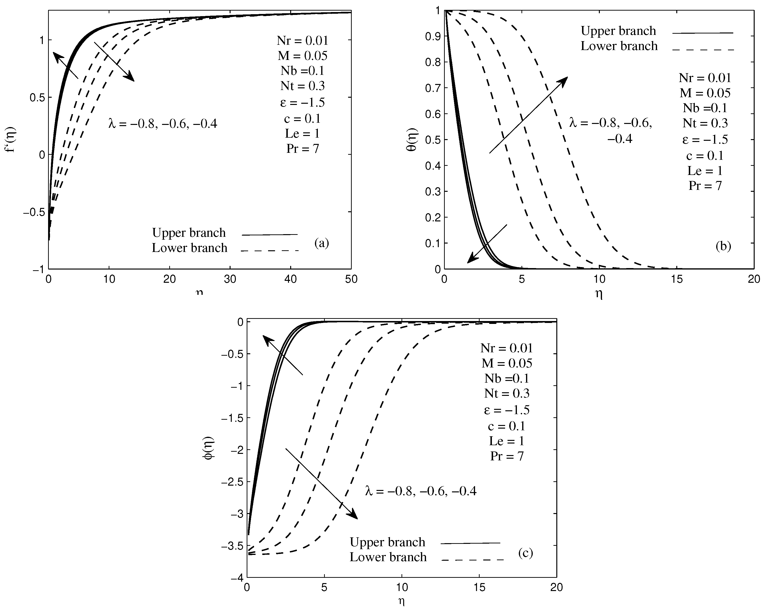
Figure 7 and Figure 8 display the variation of the velocity, temperature and concentration profiles for the influence of the magnetic field M and mixed convection parameter . As we can see, all of these profiles approach the endpoint boundary conditions Equation (10) asymptotically with various shapes, thus supporting the validity of the presents results obtained in this study. It is important to note that the existence of the dual velocity, temperature as well as concentration profiles in these figures has supported the dual nature of the solutions obtained in Figure 2 and Figure 3. As expected, the thickness of the hydrodynamic boundary layer for the lower branch solution is always thicker than the upper branch solution.
In this study, the determination of the stability of the solutions obtained is done using a stability analysis. The fact is, to perform this analysis, we must have more than one solution. The main function of this analysis is to identify which of the upper or lower branch solutions is linearly stable and physically relevant by using the bvp4c package in MATLAB software. The stability of the solutions depends on the sign of the smallest eigenvalues obtained. The unknown eigenvalue is given in Equation (24) and, to obtain the value, we must solve the linear eigenvalue Equations (25)–(27) with the respective boundary conditions Equation (28). Table 2 shows the smallest eigenvalues for different values of magnetic field and mixed convection parameter. It is clear from Table 2 that the positive value of represents an initial decay of disturbance in the boundary layer separation and the flow is said to be stable. Meanwhile, the negative value of represents an initial growth of disturbance that will interrupt the boundary layer separation, and, consequently, the flow will be unstable. It is worth knowing that the stable solution always provides a good physical meaning that can be realized. Table 2 also indicates that, as the values of are approaching , the smallest eigenvalue tends to zero either from the negative or positive side.
4. Conclusions
In the present paper, we have analyzed the boundary layer flow, heat and mass transfer of a moving vertical thin needle in an electrically conducting nanofluid. By using an appropriate similarity transformation, the governing equations are reduced to a system of coupled nonlinear ordinary differential equations which are then solved numerically using the bvp4c function in MATLAB software. The stability analysis is carried out to find the stable solutions. The findings of the present study can be summarized as follows:
- The dual solutions are more pronounced when the needle and the buoyancy forces move in the opposite direction of the free stream flow.
- The range of dual solutions is widely expanded for smaller values of magnetic parameter and the needle size.
- Stability analysis shows that the upper branch solution is stable, while the lower branch solution is unstable.
- The reduction in the magnetic parameter and the needle size will enhance the skin friction coefficients occurring between the needle and the fluid flow.
- Increasing the value of magnetic parameter, needle size and also thermophoresis parameter will definitely reduce the rate of heat transfer on the needle surface.
- The stronger rate of the Brownian motion leads to decreasing the local Sherwood number occurring on the needle surface.
Author Contributions
S.N.A.S. and N.B. designed the research; S.N.A.S. formulated the mathematical model and computed the numerical results; S.N.A.S. and N.B. analyzed the results; S.N.A.S. wrote the manuscript; S.N.A.S., N.B., N.M.A., F.M.A. and I.P. have read and approved this manuscript.
Funding
This research was funded by Putra Grant GP-IPS/2018 from Universiti Putra Malaysia.
Acknowledgments
The work of Ioan Pop has been supported from the grant PN-III-P4-ID-PCE-2016-0036, UEFISCDI, Romania. We thank the respected reviewers for their constructive comments that clearly enhanced the quality of the manuscript.
Conflicts of Interest
The authors declare no conflict of interest.
References
- Chakrabarti, A.; Gupta, A.S. Hydromagnetic flow and heat transfer over a stretching sheet. Q. Appl. Math. 1979, 37, 73–78. [Google Scholar] [CrossRef] [Green Version]
- Mahapatra, T.R.; Gupta, A.S. Magnetohydrodynamic stagnation-point flow towards a stretching sheet. Acta Mech. 2001, 152, 191–196. [Google Scholar] [CrossRef]
- Ishak, A.; Jafar, K.; Nazar, R.; Pop, I. MHD stagnation point flow towards a stretching sheet. Physica A 2009, 388, 3377–3383. [Google Scholar] [CrossRef]
- Ishak, A.; Nazar, R.; Bachok, N.; Pop, I. MHD mixed convection flow adjacent to a vertical plate with prescribed surface temperature. Int. J. Heat Mass Trans. 2010, 53, 4506–4510. [Google Scholar] [CrossRef]
- Mahapatra, T.R.; Nandy, S.K.; Gupta, A.S. Momentum and heat transfer in MHD stagnation-point flow over a shrinking sheet. J. Appl. Mech. 2011, 78, 021015-8. [Google Scholar] [CrossRef]
- Aman, F.; Ishak, A.; Pop, I. Magnetohydrodynamic stagnation-point flow towards a stretching/shrinking sheet with slip effects. Int. Comm. Heat Mass Trans. 2013, 47, 68–72. [Google Scholar] [CrossRef]
- Hakeem, A.K.A.; Ganesh, N.V.; Ganga, B. Magnetic field effect on second order slip flow of nanofluid over a stretching/shrinking sheet with thermal radiation effect. J. Magn. Magn. Mater. 2015, 381, 243–257. [Google Scholar] [CrossRef]
- Dhanai, R.; Rana, P.; Kumar, L. MHD mixed convection nanofluid flow and heat transfer over an inclined cylinder due to velocity and thermal slip effects: Buongiorno’s model. Powder Technol. 2016, 288, 140–150. [Google Scholar] [CrossRef]
- Nayak, M.K. MHD 3D flow and heat transfer analysis of nanofluid by shrinking surface inspired by thermal radiation and viscous dissipation. Int. J. Mech. Sci. 2017, 124–125, 185–193. [Google Scholar] [CrossRef]
- Lee, L.L. Boundary layer over a thin needle. Phys. Fluids 1967, 10, 1820–1822. [Google Scholar] [CrossRef]
- Narain, J.P.; Uberoi, S.M. Combined forced and free-convection heat transfer from vertical thin needles in a uniform stream. Phys. Fluids 1973, 15, 1879–1882. [Google Scholar] [CrossRef]
- Chen, J.L.S.; Smith, T.N. Forced confection heat transfer from nonisothermal thin needles. J. Heat Trans. 1978, 100, 358–362. [Google Scholar] [CrossRef]
- Wang, C.Y. Mixed convection on a vertical needle with heated tip. Phys. Fluids 1990, 2, 622–625. [Google Scholar] [CrossRef]
- Ishak, A.; Nazar, R.; Pop, I. Boundary layer flow over a continuously moving thin needle in a parallel free stream. Chin. Phys. Lett. 2007, 24, 2895–2897. [Google Scholar] [CrossRef]
- Ahmad, S.; Arifin, N.M.; Nazar, R.; Pop, I. Mixed convection boundary layer flow along vertical thin needles: Assisting and opposing flows. Int. Commun. Heat Mass Trans. 2008, 35, 157–162. [Google Scholar] [CrossRef]
- Afridi, M.I.; Qasim, M. Entropy generation and heat transfer in boundary layer flow over a thin needle moving in a parallel stream in the presence of nonlinear Rosseland radiation. Int. J. Therm. Sci. 2018, 123, 117–128. [Google Scholar] [CrossRef]
- Grosan, T.; Pop, I. Forced Convection Boundary Layer Flow Past Nonisothermal Thin Needles in Nanofluids. J. Heat Trans. 2011, 133. [Google Scholar] [CrossRef]
- Hayat, T.; Khan, M.I.; Farooq, M.; Yasmeen, T.; Alsaedi, A. Water-carbon nanofluid flow with variable heat flux by a thin needle. J. Mol. Liq. 2016, 224, 786–791. [Google Scholar] [CrossRef]
- Krishna, P.M.; Sharma, R.P.; Sandeep, N. Boundary layer analysis of persistent moving horizontal needle in Blasius and Sakiadis magnetohydrodynamic radiative nanofluid flows. Nucl. Eng. Technol. 2017, 49, 1654–1659. [Google Scholar] [CrossRef]
- Soid, S.K.; Ishak, A.; Pop, I. Boundary layer flow past a continuously moving thin needle in a nanofluid. Appl. Therm. Eng. 2017, 114, 58–64. [Google Scholar] [CrossRef]
- Ahmad, R.; Mustafa, M.; Hina, S. Buongiorno’s model for fluid flow around a moving thin needle in a flowing nanofluid: A numerical study. Chin. J. Phys. 2017, 55, 1264–1274. [Google Scholar] [CrossRef]
- Trimbitas, R.; Grosan, T.; Pop, I. Mixed convection boundary layer flow along vertical thin needles in nanofluids. Int. J. Numer. Methods Heat Fluid Flow 2014, 24, 579–594. [Google Scholar] [CrossRef]
- Salleh, S.N.A.; Bachok, N.; Arifin, N.M.; Ali, F.M.; Pop, I. Stability analysis of mixed convection flow towards a moving thin needle in nanofluid. Appl. Sci. 2018, 8, 842. [Google Scholar] [CrossRef]
- Choi, S.U.S. Enhancing thermal conductivity of fluids with nanoparticles. Am.Soc. Mech. Eng. Fluids Eng. Div. 1995, 231, 99–105. [Google Scholar]
- Wong, K.V.; Leon, O.D. Applications of Nanofluids: Current and Future. Adv. Mech. Eng. 2010, 2010, 519659. [Google Scholar] [CrossRef]
- Saidur, R.; Leong, K.Y.; Mohammad, H.A. A review on applications and challenges of nanofluids. Renew. Sustain. Energy Rev. 2011, 15, 1646–1668. [Google Scholar] [CrossRef]
- Huminic, G.; Huminic, A. Application of nanofluids in heat exchangers: A review. Renew. Sustain. Energy Rev. 2012, 16, 5625–5638. [Google Scholar] [CrossRef]
- Buongiorno, J. Convective transport in nanofluids. J. Heat Trans. 2006, 128, 240–250. [Google Scholar] [CrossRef]
- Tiwari, R.K.; Das, M.K. Heat transfer augmentation in a two-sided lid-driven differentially heated square cavity utilizing nanofluids. Int. J. Heat Mass Trans. 2007, 50, 2002–2018. [Google Scholar] [CrossRef]
- Nield, D.A.; Kuznetsov, A.V. The Cheng–Minkowycz problem for natural convective boundary-layer flow in a porous medium saturated by a nanofluid. Int. J. Heat Mass Trans. 2009, 52, 5792–5795. [Google Scholar] [CrossRef]
- Kuznetsov, A.V.; Nield, D.A. The Cheng–Minkowycz problem for natural convective boundary layer flow in a porous medium saturated by a nanofluid: A revised model. Int. J. Heat Mass Trans. 2013, 65, 682–685. [Google Scholar] [CrossRef]
- Zaimi, K.; Ishak, A.; Pop, I. Flow past a permeable stretching/shrinking sheet in a nanofluid using two-phase model. PLoS ONE 2014, 9, e111743. [Google Scholar] [CrossRef] [PubMed]
- Bachok, N.; Ishak, A.; Pop, I. Boundary-layer flow of nanofluids over a moving surface in a flowing fluid. Int. J. Therm. Sci. 2010, 49, 1663–1668. [Google Scholar] [CrossRef]
- Rashidi, M.M.; Erfani, E. The modified differential transform method for investigating nano boundary-layers over stretching surfaces. Int. J. Num. Methods Heat Fluid Flow 2011, 21, 864–883. [Google Scholar] [CrossRef]
- Rashidi, M.M.; Abelman, S.; Freidoonimehr, N. Entropy generation in steady MHD flow due to a rotating porous disk in a nanofluid. Int. J. Heat Mass Trans. 2013, 62, 515–525. [Google Scholar] [CrossRef]
- Chen, C.K.; Chen, B.S.; Liu, C.C. Entropy generation in mixed convection magnetohydrodynamic nanofluid flow in vertical channel. Int. J. Heat Mass Trans. 2015, 91, 1026–1033. [Google Scholar] [CrossRef]
- Mabood, F.; Khan, W.A.; Yovanovich, M.M. Forced convection of nanofluid flow across horizontal circular cylinder with convective boundary condition. J. Mol. Liq. 2016, 222, 172–180. [Google Scholar] [CrossRef]
- Dinarvand, S.; Pop, I. Free-convective flow of copper/water nanofluid about a rotating down-pointing cone using Tiwari-Das nanofluid scheme. Adv. Powder Technol. 2017, 28, 900–909. [Google Scholar] [CrossRef]
- Mustafa, M. MHD nanofluid flow over a rotating disk with partial slip effects: Buongiorno model. Int. J. Heat Mass Trans. 2017, 108, 1910–1916. [Google Scholar] [CrossRef]
- Hoghoughi, G.; Izadi, M.; Oztop, H.F.; Abu-Hamdeh, N. Effect of geometrical parameters on natural convection in a porous undulant-wall enclosure saturated by a nanofluid using Buongiorno’s model. J. Mol. Liq. 2018, 255, 148–159. [Google Scholar] [CrossRef]
- Weidman, P.D.; Kubitschek, D.G.; Davis, A.M.J. The effect of transpiration on self-similar boundary layer flow over moving surfaces. Int. J. Eng. Sci. 2006, 44, 730–737. [Google Scholar] [CrossRef]
- Rosca, A.V.; Pop, I. Flow and heat transfer over a vertical permeable stretching/shrinking sheet with a second order slip. Int. J. Heat Mass Trans. 2013, 60, 355–364. [Google Scholar] [CrossRef]
- Harris, S.D.; Ingham, D.B.; Pop, I. Mixed convection boundary-layer flow near the stagnation point on a vertical surface in a porous medium: Brinkman model with slip. Transp. Porous Media 2009, 77, 267–285. [Google Scholar] [CrossRef]
Figure 1.
Physical model and coordinate system.
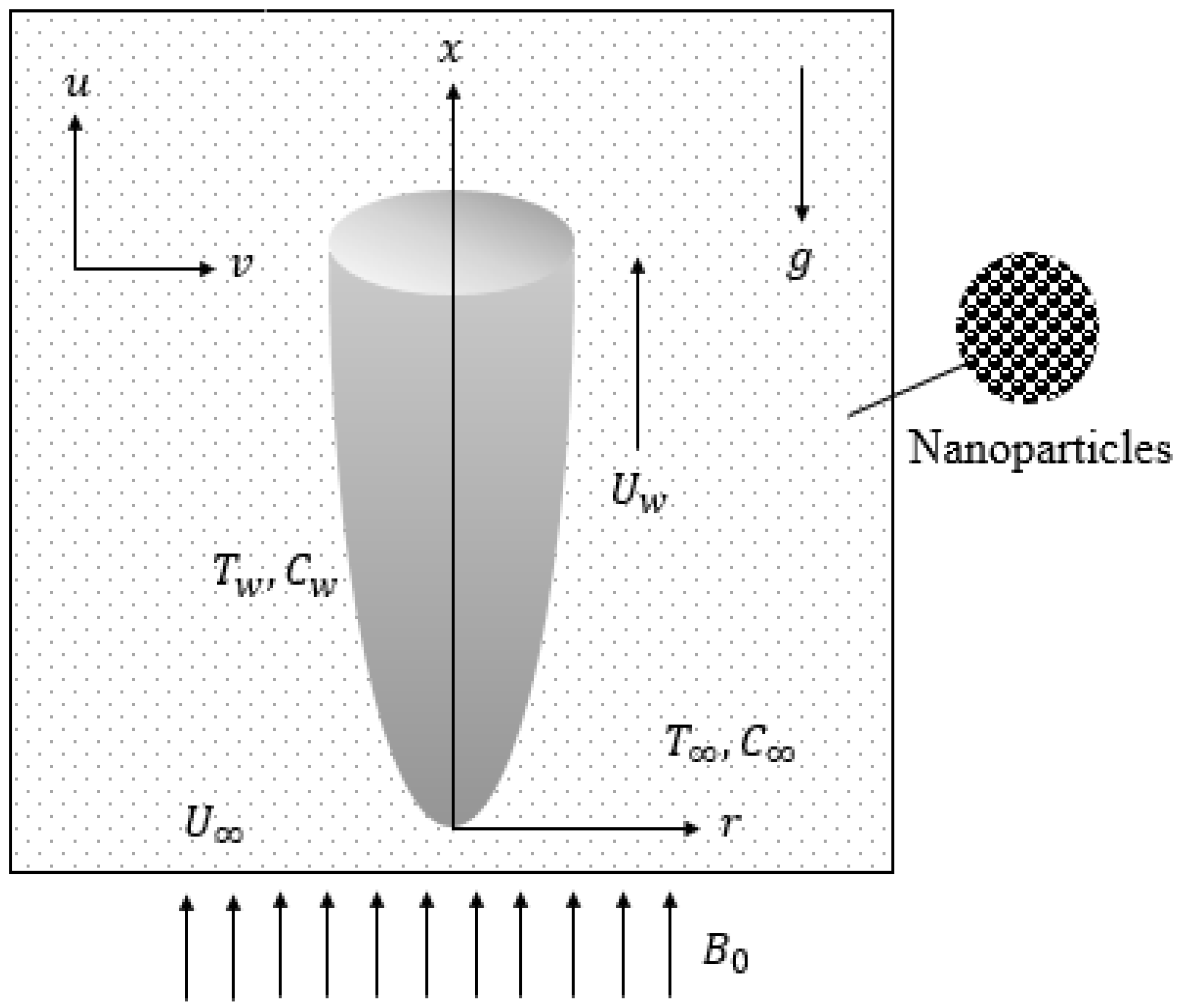
Figure 2.
Variation of (a) shear stress, (b) local heat flux and (c) local mass flux with mixed convection parameter for different values of magnetic parameter M.
Figure 2.
Variation of (a) shear stress, (b) local heat flux and (c) local mass flux with mixed convection parameter for different values of magnetic parameter M.
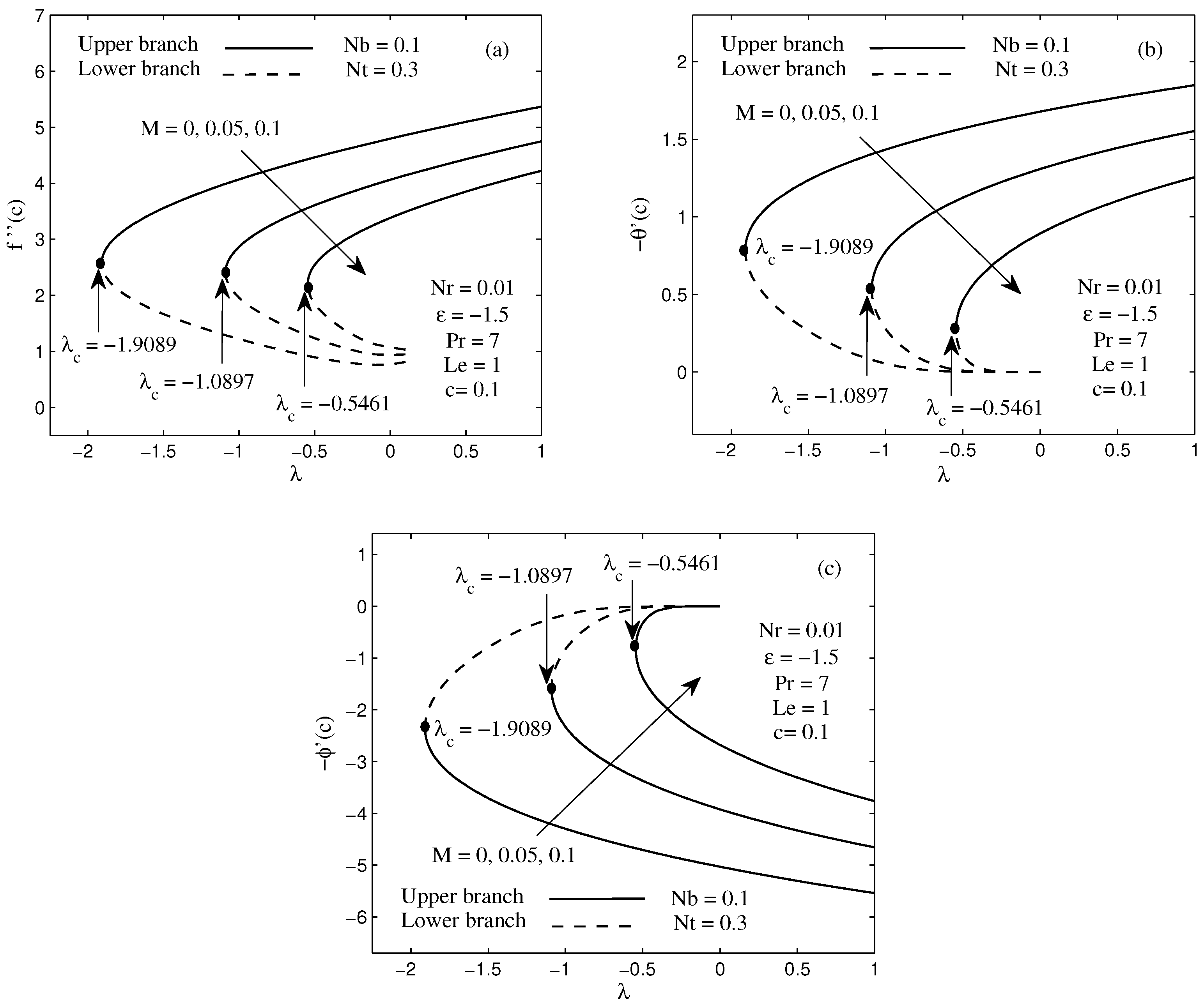
Figure 3.
Variation of (a) shear stress, (b) local heat flux and (c) local mass flux with velocity ratio parameter for different needle size c.
Figure 3.
Variation of (a) shear stress, (b) local heat flux and (c) local mass flux with velocity ratio parameter for different needle size c.
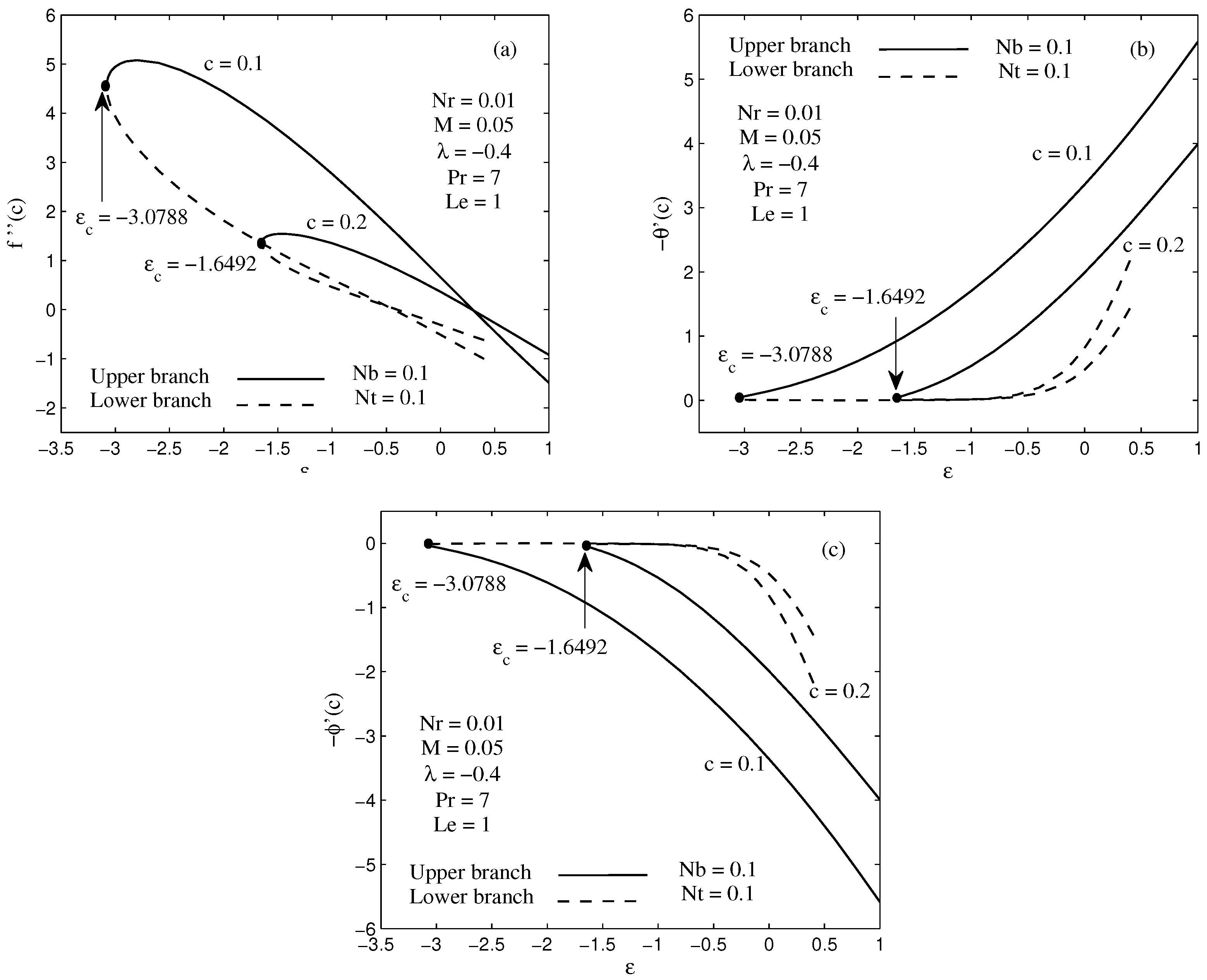
Figure 4.
Variation of skin friction coefficients with velocity ratio parameter for different values of magnetic parameter M.
Figure 4.
Variation of skin friction coefficients with velocity ratio parameter for different values of magnetic parameter M.
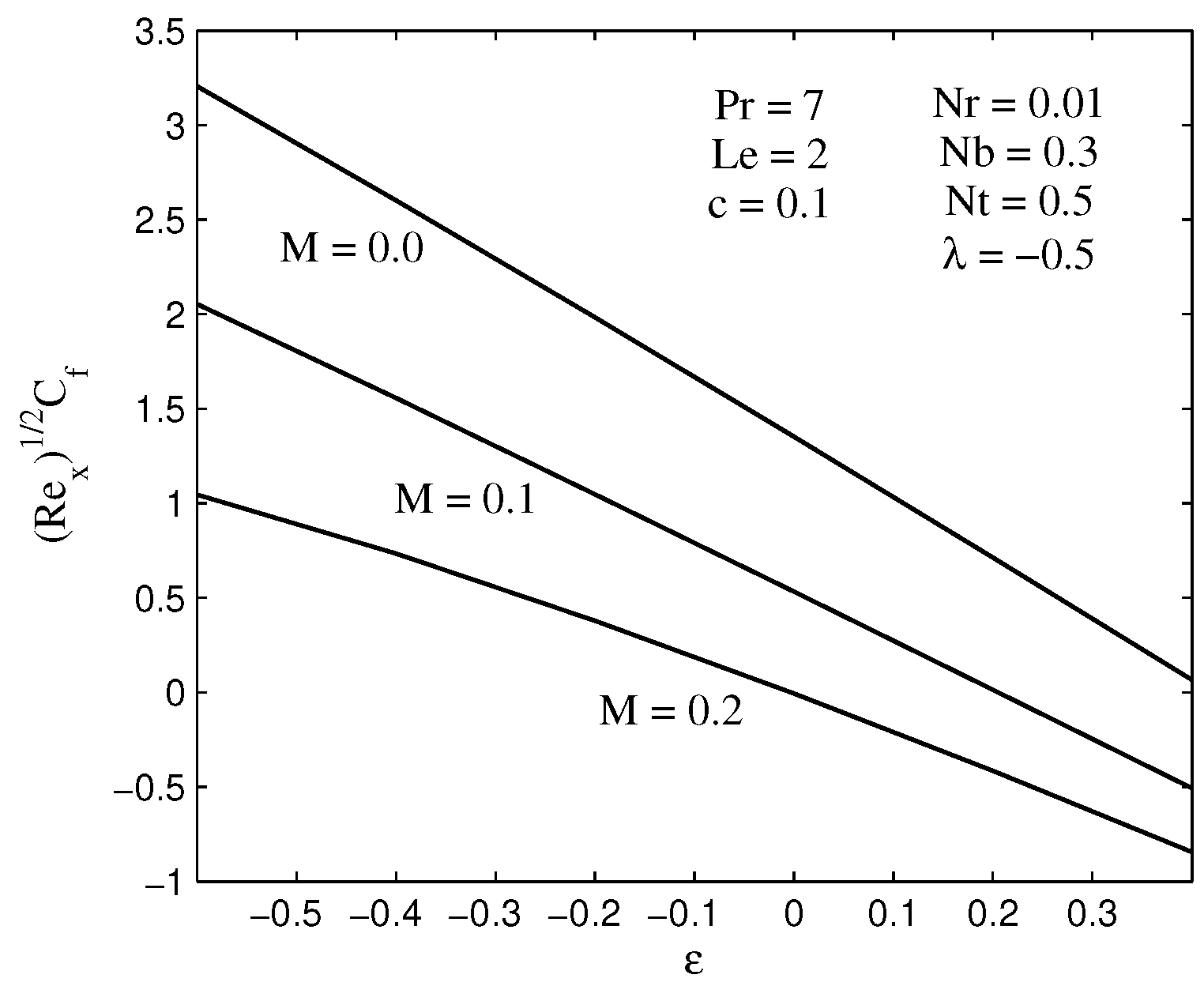
Figure 5.
Variation of local Sherwood number with thermophoresis parameter when (a) and (b) for different values of Brownian motion .
Figure 5.
Variation of local Sherwood number with thermophoresis parameter when (a) and (b) for different values of Brownian motion .
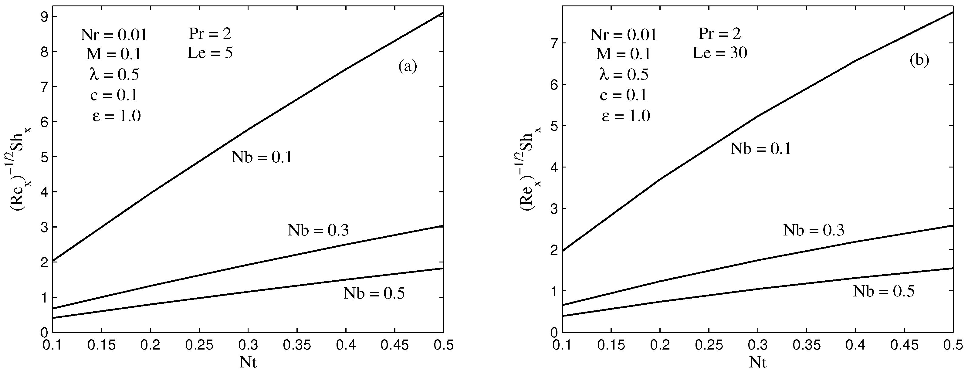
Figure 6.
Variation of (a) skin friction coefficients; (b) local Nusselt number and (c) local Sherwood number with thermophoresis parameter for different values of needle size c.
Figure 6.
Variation of (a) skin friction coefficients; (b) local Nusselt number and (c) local Sherwood number with thermophoresis parameter for different values of needle size c.
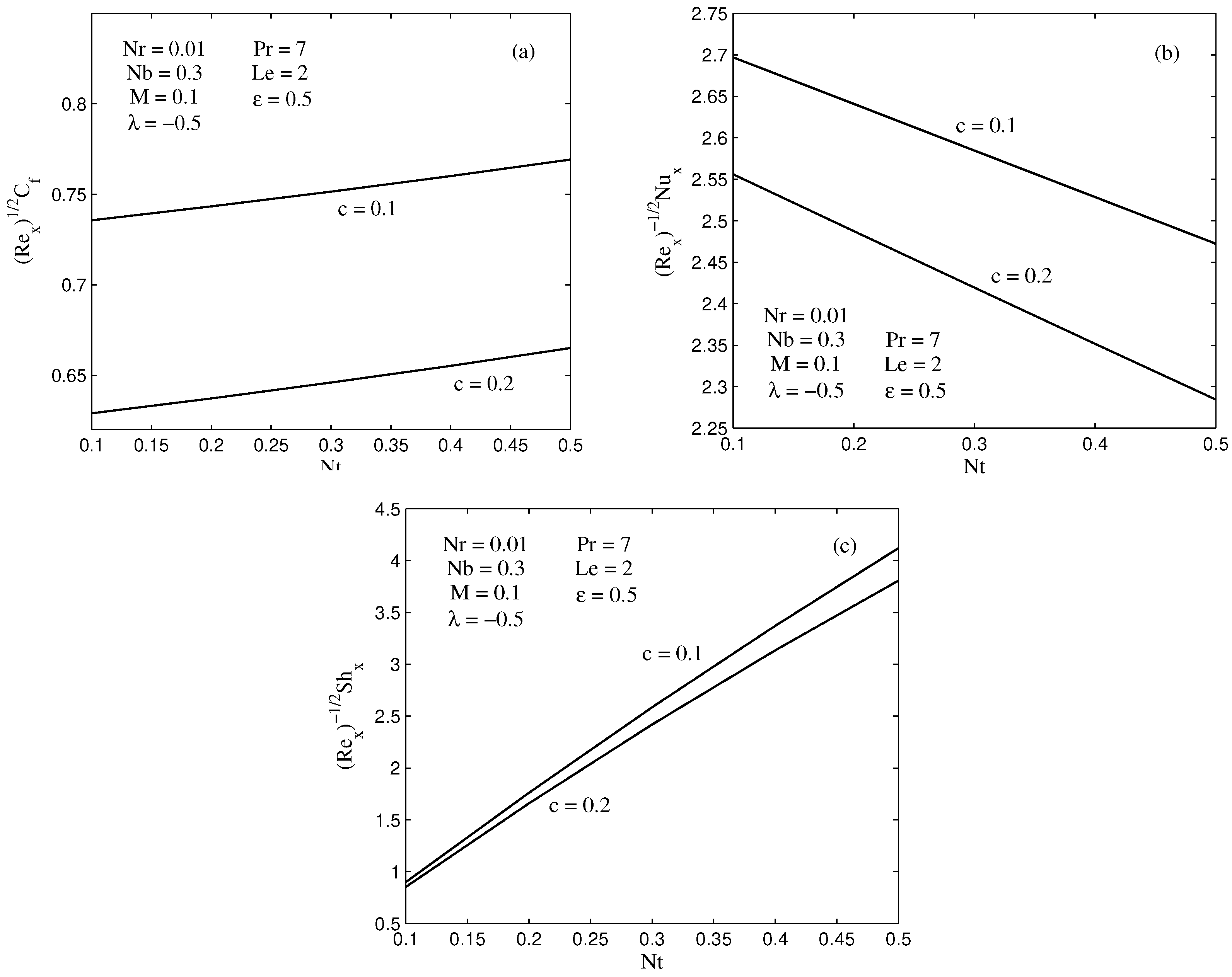
Figure 7.
Effects of the magnetic parameter M on the (a) velocity profiles; (b) temperature profiles; and (c) concentration profiles.
Figure 7.
Effects of the magnetic parameter M on the (a) velocity profiles; (b) temperature profiles; and (c) concentration profiles.

Figure 8.
Effects of the mixed convection parameter on the (a) velocity profiles; (b) temperature profiles; and (c) concentration profiles.
Figure 8.
Effects of the mixed convection parameter on the (a) velocity profiles; (b) temperature profiles; and (c) concentration profiles.

Table 1.
Numerical values of when and for some values of needle size c.
| c | Ahmad et al. [21] | Present Work |
|---|---|---|
| 0.1 | 1.2888171 | 1.2888299 |
| 0.01 | 8.4924360 | 8.4924452 |
| 0.001 | 62.163672 | 62.163606 |
Table 2.
Smallest eigenvalues for some values of magnetic field M and mixed convection when , , , , and .
Table 2.
Smallest eigenvalues for some values of magnetic field M and mixed convection when , , , , and .
| M | Upper Branch | Lower Branch | |
|---|---|---|---|
| 0 | −1.8986 | 0.0301 | −0.0291 |
| −1.898 | 0.0309 | −0.0299 | |
| −1.89 | 0.0410 | −0.0392 | |
| 0.05 | −1.0864 | 0.0173 | −0.0169 |
| −1.086 | 0.0184 | −0.0179 | |
| −1.08 | 0.0299 | −0.0286 | |
| 0.1 | −0.5448 | 0.0111 | −0.0108 |
| −0.544 | 0.0141 | −0.0137 | |
| −0.54 | 0.0243 | −0.0230 |
© 2018 by the authors. Licensee MDPI, Basel, Switzerland. This article is an open access article distributed under the terms and conditions of the Creative Commons Attribution (CC BY) license (http://creativecommons.org/licenses/by/4.0/).
Share and Cite
MDPI and ACS Style
Salleh, S.N.A.; Bachok, N.; Arifin, N.M.; Ali, F.M.; Pop, I. Magnetohydrodynamics Flow Past a Moving Vertical Thin Needle in a Nanofluid with Stability Analysis. Energies 2018, 11, 3297. https://doi.org/10.3390/en11123297
AMA Style
Salleh SNA, Bachok N, Arifin NM, Ali FM, Pop I. Magnetohydrodynamics Flow Past a Moving Vertical Thin Needle in a Nanofluid with Stability Analysis. Energies. 2018; 11(12):3297. https://doi.org/10.3390/en11123297
Chicago/Turabian StyleSalleh, Siti Nur Alwani, Norfifah Bachok, Norihan Md Arifin, Fadzilah Md Ali, and Ioan Pop. 2018. "Magnetohydrodynamics Flow Past a Moving Vertical Thin Needle in a Nanofluid with Stability Analysis" Energies 11, no. 12: 3297. https://doi.org/10.3390/en11123297
Note that from the first issue of 2016, this journal uses article numbers instead of page numbers. See further details here.