An Integration Mechanism between Demand and Supply Side Management of Electricity Markets


1
School of Computer Science, University of Manchester, Manchester M13 9PL, UK
2
BRE Trust Center for Sustainable Engineering, Cardiff University, Cardiff CF24 3AA, UK
*
Author to whom correspondence should be addressed.
Energies 2018, 11(12), 3314; https://doi.org/10.3390/en11123314
Submission received: 13 October 2018
/
Revised: 20 November 2018
/
Accepted: 23 November 2018
/
Published: 27 November 2018
(This article belongs to the Special Issue Demand Response in Electricity Markets)
Abstract
:One of the main challenges in the emerging smart grid is to jointly consider the demand and supply, which is also reflected in the wholesale market (supply side) and the retail market (demand side). When integrating the demand and supply side into one framework, the mechanism for determining the market clearing price has been changed. This is due to the demand variations in the demand side in response to the market clearing price and the change of generation costs in the supply side from the demand variation. In order to find the best balance between the supply and demand under the demand response management scheme, this paper proposes a new integrated supply and demand coordination mechanism for the electricity market and smart pricing methods for generator and retailers. Another important contribution of this paper is to develop an efficient algorithm to find the match equilibrium between the demand and supply sides in the new proposed mechanism. Experimental results demonstrate that the new mechanism can effectively handle unpredictable demand under dynamic retail pricing and support the ISO to dispatch the generation economically. It can also help in achieving the goals of dynamic pricing such as maximizing the profits for retailers.
1. Introduction
Since the early 21st century, the traditional electricity grid has been restructured and replaced by the Smart Grid (SG) in many countries [1,2]. However, the better infrastructure does not make the grid ‘smart’ automatically. One of core technologies that make the grid ‘smart’ is called demand response (DR). DR is designed to control the demand of electricity on the customer’s side where they could incentivize customers to reduce consumptions in peak demand periods or shift consumption from peak demand periods to off-peak demand periods. With the help of smart meters [1,3], customers will benefit from DR programs by actively managing their demand. A lot of literature has demonstrated that the DR program could bring benefits not only for customers but also for generators and retailers [4,5,6,7,8,9,10] in such that shifting of the demand could flatten the aggregated demand profile and hence reduce the total production cost.
Unlike other products, electricity cannot be stored in stock. To guarantee a reliable supply of electricity for industries and customers, the supply and demand must be balanced at any given time. Therefore, a coordination agency, the Independent System Operator (ISO) [11,12], is needed in order to coordinate the dispatch of generation units and meet the expected demand of electricity across the transmission grid [13]. However, the implementation of DR programs will result in the mismatch integration problem between retail and wholesale the electricity markets, which is caused by the elastic demand from customers—the customers under DR will respond to the retailer’s pricing signal which leads to a new demand (unpredictable of demand-side). On the one hand, this mismatch integration problem will prevent the retailer from determining the proper retail prices and the quantity of electricity it should buy from the wholesale market. On the other hand, without knowing sufficiently accurate demand, it is very difficult for the ISO to schedule the generations efficiently for the wholesale market. As a result, in that situation, a lot of real-time balancing and reserve energy resources are required to guarantee the security of supply in the system, which leads to a lower social welfare for the energy system and is much undesirable.
Most of existing studies consider the demand and the supply side separately. The studies focusing on demand side within the retailer market usually take advantage of the historical smart meter consumption data to build customers’ demand models. After obtaining customers’ demand models, retailers can obtain optimal pricing for their customers and decide how much electricity they should buy from the wholesale market. For instance, Ma and Zeng [14] used historical consumption data to build consumers’ demand models with a matrix of self- and cross-elasticities. This matrix reflects the reaction of customers’ demand to electricity prices. They showed that, with the help of this matrix, the retailers can optimally price the electricity to maximize their profit. Aalami et al. [9,15] proposed a new demand response modelling based on the price elasticity of demand and benefit function of customers. By using this model, the ISO can simulate the behaviour of customers under relevant DR program. Maharjan [16] modeled a retailer and its customers as a Stackelberg game. Within this game, the objective of each player is to maximize its own profit. A distributed algorithm is developed which converges to the Stackelberg equilibrium with using only the local information about the retailer and customers. In [17], Bu and et al. modeled and analyzed the interactions between the retailer and its customers as a four-stage Stackelberg game, in which the customers’ preferences and electricity consumption patterns are modelled via various utility functions. In [18], Chen et al. proposed an optimal demand response scheduling scheme based on Stackelberg game while considering the load uncertainty.
On the other hand, there are studies focusing on the supply side that usually only consider the interactions between the generators and ISO to determine optimal generation schedules to meet demand with assumption that customers’ demand is relatively stable and predictable where an integration mechanism between the retail and wholesale market considering demand response is still missing in the existing studies. For instance, Farqui et al. discussed that serval demand response programs such as dynamic pricing and other time-based pricing rates can be introduced in the wholesale markets run by ISO [19]. Kirschen et al. [4] used historical consumption data to model consumers’ demand model as a matrix of self- and cross-elasticities. With the help of this matrix, the ISO can efficiently schedule the supply and power generation to limit electricity abuse and wastage. Su and Kirschen [6] designed a new centralized complex-bid market-clearing mechanism which can determine the optimal production and consumption schedule to maximize the social welfare. The mechanism has considered the effect of demand shifting and shown that demand shifting improves the economic efficiency of the market.
Although the above studies have provided valuable insights, there are two limitations that still need to be overcome: Firstly, due to the mismatch between the ISO’s estimated demand and actual demand under the retailers’ pricing schemes, the supply and demand cannot be balanced efficiently in real-time by the ISO (i.e., a lot of balancing and reserve energy resources are needed, which is inefficient). In the existing research, each retailer provides the elasticity matrix to the ISO or the ISO estimates the customers’ demand preference based on past data. Then the ISO based on this matrix or the estimated customers’ demand model in order to estimate the demand and calculate the MCP. However, the retailers’ pricing methods in the retail market are obviously different from the ISO and usually unknown to the ISO, which makes the ISO’s modelling of demand inaccurate. For instance, after having received the MCP from the ISO, the retailers will reprice the electricity based on their own pricing considerations and methods. Under the retailers’ announced dynamic prices, the response from customers could lead to a completely different demand from the ISO’s estimation, and result in a huge mismatch between the actual demand and the estimated demand from ISO. To balance the demand and supply, the new arisen demand will pose threats to the security of supply or require a lot of real-time balancing and reserve resources, which is undesirable and much less efficient. That is, the current wholesale market mechanism cannot handle the unpredictable demand introduced by demand response programs. As a result, an energy market integration mechanism which links both the demand-side and the supply-side with considering demand response is urgently needed. Secondly, all the above existing studies assume that a retailer’s total cost is a function (such as [14,15,17,18,20], most are quadratic functions) which only depends on its own demand rather than the demand of all retailers. However, the unit cost (MCP) and the total cost is based on the demand of all retailers in reality, which means that the change of one retailer’s demand could change all retailers’ unit costs and the total cost. Therefore, the current retail pricing mechanisms will not work properly especially when we integrate the wholesale market and the retail market into one framework.
It is obvious from the above analysis that the existing studies and market mechanism, which separates the demand and the supply side management, could not account for the mismatch integration problem introduced by demand response programs. As a result, an energy market integration mechanism to consider both the retail market and wholesale market with demand response is needed. There are only limited studies consider both the demand-side and supply-side into one framework with demand response. Furthermore, the current market structure and operation mechanism (e.g., double auction for market clearing) of the wholesale market is usually not considered in existing studies. For instance, Yu et al. [21] proposed a novel incentive-based demand response model from the view of the grid operator to enable system-level dispatch of demand response resources. In this model, the effect of demand response can be appropriately reflected in the whole system where a two-loop Stackelberg game is modeled to capture the hierarchical interactions among different groups including generators, grid operator, energy service provides and end consumers. However, same as other existing studies of this kind, Yu et al. [21] mainly focuses on integrating the demand response into the whole energy system in order to induce the demand reduction in the retail side and cost minimization in the generation side, rather than balancing the demand and supply based on the current structure of the electricity market.
To overcome the above limitations, in this paper we propose a new market integration mechanism to integrate and balance the demand and the supply to address the challenges of unpredicted demand due to dynamic pricing and demand response management programs. The main contributions of this paper are summarized as follows:
- Different from the existing market mechanism where the ISO only declares a single demand in the wholesale market, in our mechanism, the ISO declares a demand interval to the wholesale market for each hour. The demand interval is easy to estimate and more robust than a single demand and enables the ISO to handle unpredictable demand under the DR programs in our mechanism.
- The proposed mechanism also enables the ISO to realize the goals of dynamic pricing and demand response by utilizing smart meters such as effectively reducing CO2 emission, minimizing bills for customers and maximizing the profit for both retailers and generators. The related smart pricing methods for the retailer are also proposed in the context of this new market integration mechanism.
- An efficient algorithm is proposed to find the match equilibrium between the demand and supply side for the proposed new integration mechanism. Moreover, a formal proof process is also provided in this paper, which shows that the proposed algorithm and mechanism are effective and valid for the real market.
The rest of this paper is organized as follows: In Section 2, we illustrate the problem statement and the methodology which is applied to solve the problem. Then the proposed market model is presented in Section 3, Section 4 and Section 5 in detail. After that, numerical results are given in Section 6. This paper is summarized in Section 7.
2. Problem Description
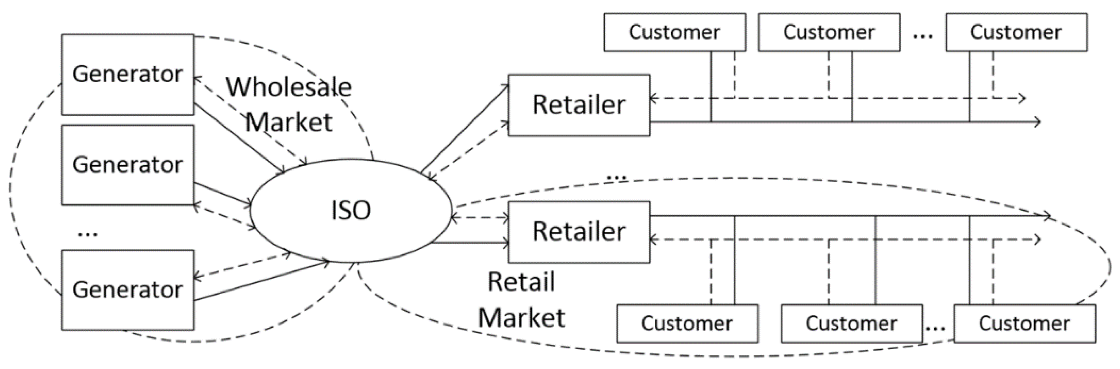
The structure of the electricity market that we consider in this paper is shown in Figure 1. Similar with [22,23] and [21], the electricity market consists of several generators, ISO, several retailers and many customers. The ISO acts as the coordinator between the wholesale and the retail markets by determining the MCP and scheduling the power generation to meet the required demand of the retailer market.
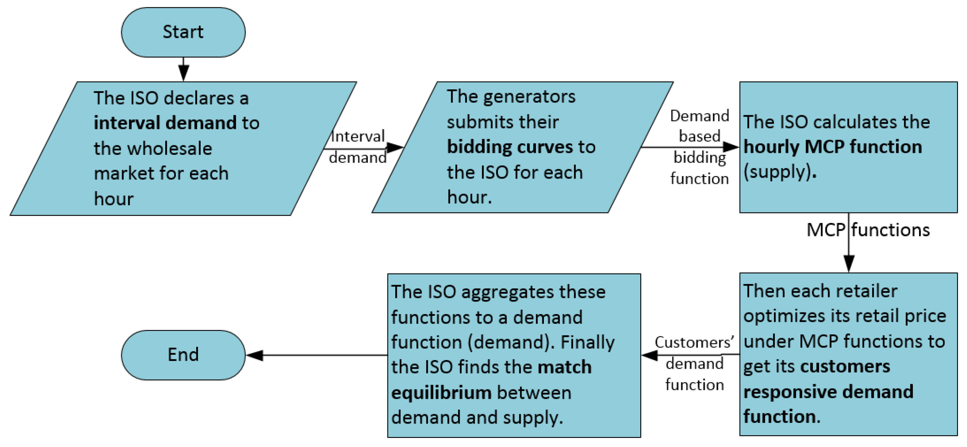
Given the above electricity market, the working process of the proposed mechanism is presented as follows: firstly, facing the difficulty of unpredictable demands, the ISO declares a demand interval to the wholesale market for each hour. Knowing the interval demand, each generator decides its bid curve of each hour. After receiving the bid curve of each hour from each generator, the ISO generates the aggregated MCP supply curve (MCP function) for each hour and sends these to retailers. Based on hourly MCP functions, the retailers decide their optimal prices for their customers. Then the total customers’ demand function, which is a function of the MCP, can be obtained by the retailer and sends them respectively to the ISO. The ISO then aggregates these functions from retailers to a total demand function which is dependent on the MCP. Finally, the ISO finds the demand match equilibrium between demand and supply and use the corresponding MCP as the final MCP of the proposed mechanism. The working process of the proposed new mechanism is also presented in Figure 2 and each step within this process is described briefly as follows:
- Step 1. ISO declares the demand interval of each hour of the next day to all the generators:
Different from the existing practice in which ISO declares a predicted demand figure of each hour of the next day to all the generators, the declared demand interval in the new mechanism avoids the difficulty of the unpredictable demand under the DR programs. Such a demand interval only needs to be determined wide enough to cover all the possible demands of each hour in the next day, such as the min and max demand of each hour from the historical data plus any possible variation due to the other factors such as weather conditions or other events. The benefit of using demand intervals is that it is more robust than a single demand figure and enables the ISO to handle unpredictable demand under the DR programs.
- Step 2. Each generator decides its hourly bid curve, based on the declared demand interval from ISO:
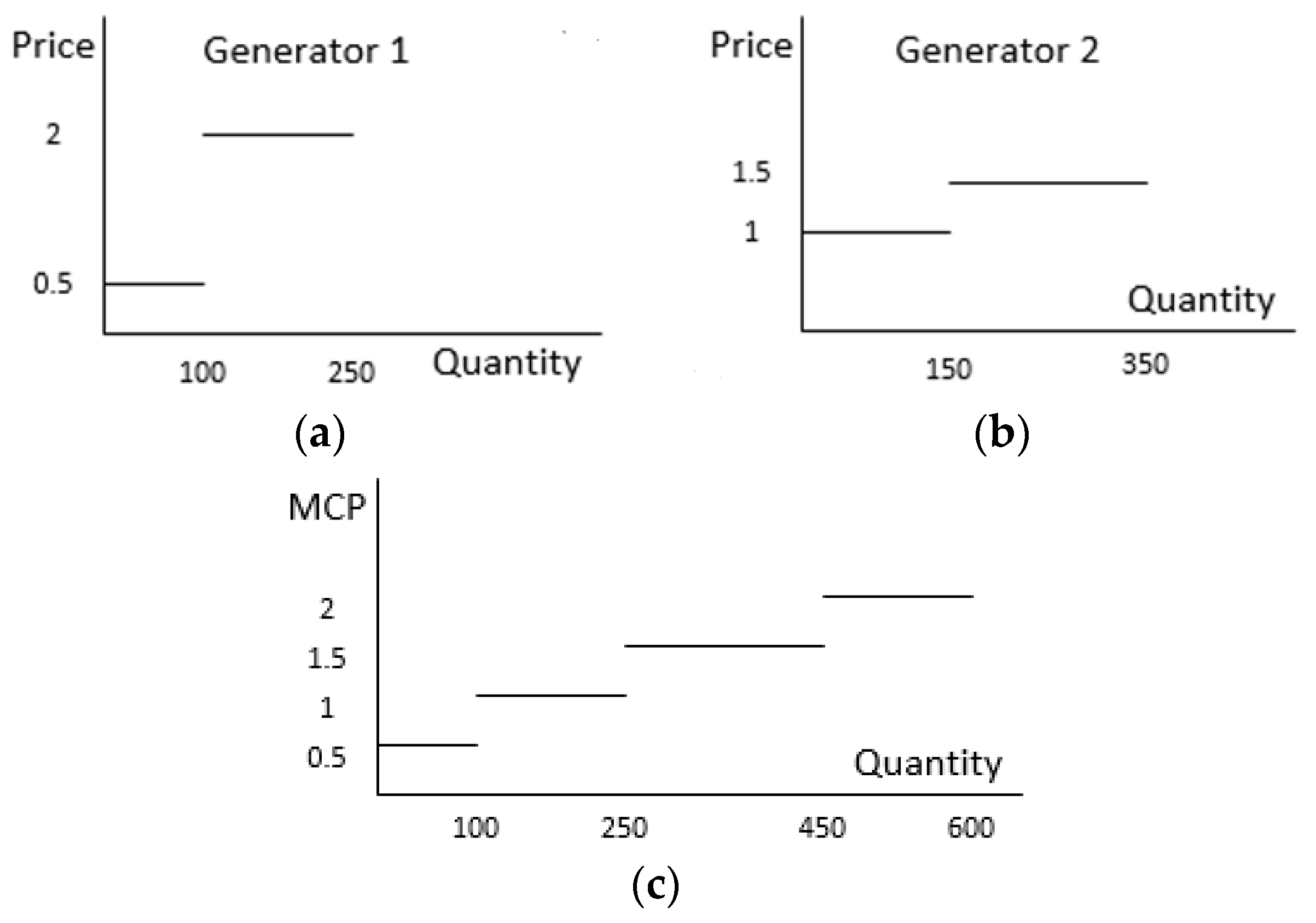
Different from the existing practice where each generator decides a single value of supply and the corresponding price as its bid based on a single demand figure from ISO [6,24], each generator will submit a hourly bid or supply curve based on the interval demand announced by ISO. Such a bid supply curve of a generator usually is a piecewise constant and monotone increase function with the bid quantity as the input variable and the bid price as the output variable, as shown in Figure 3 (e.g., see Generator 1). To address the problem of how to generate the bid curves for a generator within the proposed mechanism, we have proposed a neural network approach to predict the winning curves in [25]. Therefore, this problem will not be further discussed in this paper.
- Step 3. After receiving the bid curve from each generator, the ISO calculates the aggregated bids curve (step function) for each hour.
This hourly-aggregated bid curve is the calculated hourly MCP. The most important feature of this MCP is that it is a function which is dependent on demand. This is different from the current work in which the calculated MCP is a single value and not dependent on the demand (as the demand is just a one number in that case). Each MCP function consist a set of supply segments and the corresponded MCP. This MCP function can directly reflect the MCP with a minimum production cost under the demand from the retailers. The Figure 3 shows an example to explain the process of Step 3. The problem is that how to generate a MCP curve under generators’ submitted bids for each hour. An algorithm is proposed to solve this problem, which is presented in Section 3.
- Step 4. Based on hourly MCP functions, the retailers decide their optimal prices for their customers. Then the total customers’ demand function, which is a function of the MCP, can be obtained by the retailer and sent back respectively to the ISO.
For the retail market, we consider that each electricity retailer has its own customers in the market as shown in Figure 1 and the day-ahead dynamic pricing is applied. The customers consume the next day’s electricity depending on the announced price, and their preference is to maximize their utility (such as minimizing their bills, or maximizing the convenience, or combining both). In our new mechanism, the ISO sends hourly MCP functions to all retailers. Since each MCP function is a step function which consist of a set of segments, each segment is a price with a lower and upper bound of corresponding supply quantity. Then the retailer can obtain a set of MCP vectors for 24 h: = , in which for any hour , . By using the estimated customers’ reaction function learned from historical demand and pricing data and basing it on each MCP vector for the next day, the retailer determines the 24-h prices for the next day in order to maximize its profit. Each MCP vector is then matched with a customers’ demand vector. Then customers’ demand function which is a function of the MCP can be obtained by the retailer and sent to the ISO. This is different from current mechanisms which only calculate a single vector of 24 values for the demand. The main problem for the demand side is the retailer’s pricing problem. That is, how to price optimally in order to maximum the profit under each MCP vector for the retailer. A solution is provided in Section 4.
- Step 5. After receiving the customers’ demand function from each retailer, the ISO aggregates these functions to a demand function which is dependent on the MCP. Based on the obtained MCP functions and demand function, the next step of the proposed mechanism consists of the ISO finding the balance points between the demand and supply. The balance points in each hour of the next day are the proposed result of this mechanism.
As aforementioned, because of demand response, the customers will usually react to dynamic retail prices, which will lead to a new demand different from the expected or predicted by the ISO/retailers. According to the definition, the balance point in each hour means that the customers’ ultimate demand under the dynamic retail prices (the amount of electricity that the customers buys from their retailers in the retail market) and the supply from the wholesale market in this hour (the amount of electricity that the generators sells to the retailers in the wholesale market) are located in the same segment in the MCP function, which indicates that they have the same unit cost for the retailer. Since the unit cost is unchanged in the retail market, the retailer’s optimal pricing model is deemed to be successful after integrating the demand side with the supply side. However, without our integration mechanism, the ISO’s aim of balancing supply and demand will fail due to its incapability of handling the effects of demand response in the market. That is why finding the match equilibrium is so important for the ISO when integrating the demand and supply side into one framework. As a result, in this paper we propose a new integration mechanism for the ISO to efficiently find the match equilibrium between the supply and the demand and an analytical optimization method is presented to attain the match equilibriums, which are given in Section 5.
3. Generation Side
In this section, the method of how the ISO obtains the MCP function in the wholesale market is illustrated.
In the proposed new mechanism, the first step involves the ISO declaring a demand interval to the wholesale market for each hour as we showed in Figure 2. Then, based on the informed hourly demand interval, each generator submits its bid curve (a set of bid segments which is sorted by the bid price in the increasing order: (), where is the bid price of -th segment of generator ’s bid curve in hour h, and is the lower and upper bound of supply of this segment.) to the ISO for each hour. At the third step of our mechanism, the ISO uses Algorithm 1 to aggregate all the bidding curves to a supply curve of hour h and, based on this bidding curve, the ISO obtains a MCP function in hour h. In order to reach the requirement of economic dispatch, the production cost on the generation side should be minimized and the demand from the retailer should be fulfilled. Therefore, the MCP functions should minimize the production costs under any amount of demand. Algorithm 1 shows how we get the MCP function for hour h. In Algorithm 1, is the number of generators; is the number of total segments in all generators’ bidding curves of this hour; is the number of total segments of all generators’ bidding curves in hour h, where ; is the k-th segment of the proposed step function in hour h; is the corresponding unit price of ; is the corresponding supply quantity of . Then the ISO aggregates all the bidding curves to a supply curve of hour h. This supply curve represents a MCP function in that hour. In order to reach the requirement of economic dispatch, the ISO should minimize the production cost of the dispatched generation and fulfill the demand from the retail market. Therefore, the production cost should be minimized under any amount of demand in each hourly MCP function. Algorithm 1 shows how the ISO obtains the MCP function for hour h. Through using Algorithm 1, the ISO can obtain the MCP function (1) for each hour and sends these functions to all retailers. is the demand from the retail market in hours:
In Algorithm 1, the ISO sorts all bids segments of all generators’ bidding curves in the increasing order by the unit price and then starts from the smaller one in order to put them into the aggregated bidding curve. The segments in the aggregated bidding curve are also ordered in increasing order, which means that the amount of electricity which has the lowest unit price is always dispatched first. Therefore, we can say that the MCP functions minimize the production cost under any amount of demand. Then the ISO transfers the obtained MCP functions to the format of Table 1. Table 1 is the MCP table with the corresponding supply segments under all MCP functions. For each hour h, we use to present the maximize number of segments in the MCP function of hour h (for any two different hours i and j in , could be different to ).
| Algorithm 1 Calculate the MCP function of hour h | |
| Input: Each generator’s bid curve of hour h: generator i’s bid curve can be represented as a set of bid segments () sorted by the bid price in the increasing order; | |
| Output:MCP function of hour h; | |
| 1: | For each generator , get the unit price and the corresponding quantity bids () of each segment in the generator i’s bidding curve of hour h. |
| 2: | Let be the ordered unit prices of all segments in generators’ bidding curves and be the corresponding quantity bids , where is the number of total segments in all generators’ bidding curves. |
| 3: | Assigns the value of and to and respectively, assigns and to the lower and upper bound of respectively. |
| 4: | Fork = 2 to do |
| 5: | Assigns the value of and to and respectively; assign to the upper bound of and assign the value of upper bound of to the lower bound of . |
| 6: | End for |
| 7: | A new set of segments () is obtained, which can be plotted as a step function in the coordinate system. This new step function is the MCP function in hour h (Equation (1)). |
4. Retailer’s Pricing Optimization
In this section, we describe the details of the retailer’s optimal pricing model.
As stated before, we assume that all households have installed the smart meter. This means that historical price and demand information in the retail market are available for the retailer. Through using Ma’s learning method in [10], we can model customers’ consumption behaviors by estimating the customer’s reaction function. The form of estimated reaction function for each hour can be represented as:
The represents the cross-elasticity coefficients which relate the responsiveness of the customers’ demand for the electricity at hour to a change in the price of electricity during other hours. For instance, when the price of electricity at hour increases but prices at other times remain unchanged, some demand at hour will be shifted to hour , and therefore the demand at hour increases. Thus, cross-elasticity is usually greater than 0. In contrast with the cross-elasticity, self-elasticity coefficient means the relationship between the demand in hour h and the price of that hour. That is, when the price at hour increases but prices at other times remain unchanged, the demand at hour decreases, and thus the self-elasticity is usually less than 0.
The parameters in the Equation (2) are unknown and one can use historical price and demand data to estimate the above parameters. As described in [14], this problem can be formulated as a quadratic programming problem, which can be solved in Matlab with existing solvers.
After obtaining the customers’ demand model, the next step is to solve the optimal pricing problem for the retailer under certain constrains. In the following part of this section, we will introduce the retailer’s optimal pricing model.
In our model, each retailer sets optimal prices for its customers in order to maximize its own profit after receiving the MCP vector. Normally the retailers in the market are always competitive in-between. However, as we are discussing the pricing for next day and the competition which exists within a day can be ignored. This is because the customers switching within one day is very limited, and thus can be ignored. Therefore, retailers are pricing independently and there is no cross-impact between the prices of different retailers in this scenario, meaning that each retailer has its own customers. That is, we do not consider the competition among retailers with 24 h in this model. If needed, a retailer can set price differential bounds with its competitors to take the competitive impact of prices into consideration.
For each hour , the minimal and maximal retail price constraints are set as follows:
If the retailer set its price in each hour h equal to in order to maximize its profit, then its customers would also have no options to reschedule their demands. Thus, we set the constraint on the retailer’s total revenue:
Finally, we can express the retailer j’s optimal pricing problem as problem (5):
where is retailer j’s optimal retail price in hour ; is the demand from the retailer j’s customers in hour ; is the profit of retailer j. Given an MCP vector (consists of ), the retailer j can find the best prices for maximizing its profit by solving the optimization problem in Equation (5). As this is a quadratic programming problem, it can be solved with the SCIP solver from Matlab OPTI TOOLBOX.
It should be noted that in our mechanism, the retailer receives the hourly MCP function from the ISO. This means that the in Equation (5) is not a number but a function like showed as Equation (1). Therefore, the solution of problem in Equation (5) will be dependent on each of MCP function in hour h, which is much more complicated to solve than before. That is, based on the hourly MCP functions, the retailer obtains a set of MCP vectors for next 24 h, which includes all possible combinations of MCP vectors. Then each retailer optimizes its retail price under each MCP vector for the next 24 h where each MCP vector is then matched with a customers’ response vector. Thereafter, the customers’ demand function which is dependent on the MCP vector, can be obtained by the retailer and sent to the ISO, i.e., . After that, the ISO aggregates these demand functions to an aggregated demand function. Finally, the ISO finds the match equilibrium between the demand and supply as a result of the proposed mechanism where the details of how the ISO finds the match equilibrium between demand and supply are illustrated in the next section.
5. Balancing the Demand Side and Supply Side
In this section, we introduce our new analytical optimization method to solve the mismatch integration problem. This method can accurately find the match equilibrium in order to best balance the supply and demand. In the first sub-section, the definition of match equilibrium will be introduced. Then we will illustrate the detail of the new analytical optimization method in the second sub-section.
5.1. Match Equilibrium
The methods involving how to obtain the MCP function on the supply side and how to find the optimal prices in order to maximize the profit for the retailer on the demand side have been discussed and solved in the previous sections. However, in the existing wholesale pricing mechanism, the supply and the demand under the demand response program cannot always be matched as aforementioned. In order to overcome this problem, we will illustrate our new analytical optimization method which can efficiently find the match equilibrium between supply and demand in this subsection.
Recall that in the fifth step of our mechanism as shown in Figure 2, the ISO wants to find the match equilibriums between demand and supply for each hour of the next day. Here we firstly define the match equilibriums.
Definition 1.
Denote the MCP vector obtained by the ISO from allfunctions (Equation (1)) as . If MCP satisfies the following condition (6), it is said that the demand and supply reach the match equilibrium under this MCP vector proposed by ISO.
In Equation (6), is the demand of all retailers in hour h under , where is equal to the demand of retailer j’s customers: which can be calculated by solving optimization problem (5); and are the lower and upper bounds of corresponding supply segment in Table 1 respectively.
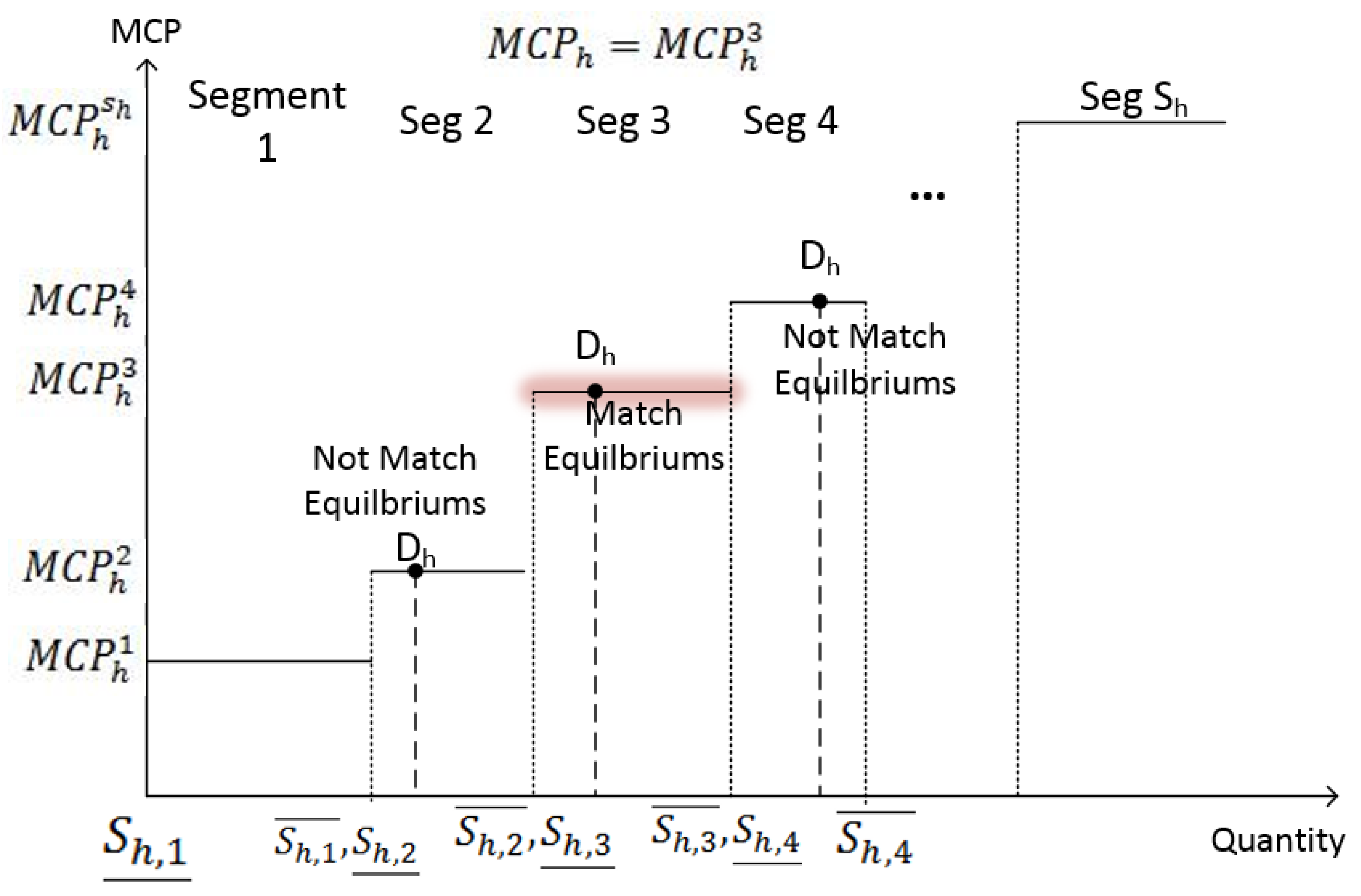
Under the match equilibrium, the total customers’ demand of hour h: is located within the supply segment: (, ] in Table 1 when the market clearing price is . Therefore, the balance of supply and demand is matched and then avoids the shortage and surplus of electricity. Figure 4 shows an example of match equilibrium in hour h.
Although the MCP functions are already known, finding the match equilibrium between the demand and supply for each hour of the next day remains a complicated problem for the ISO. This is because the combination of MCP vectors for the next day amounts to a really large number. For each hour h, we use to present the maximize number of segments in the MCP function (Equation (1)) at hour h. The domain of in the MCP function is . Then the combination of all possible MCP vectors in the next day is equal to . For example, when both of are equal to 3 and H is equal to 24, the numbers of combination of all MCP vectors for the next day is 2.8243 ×10¹¹. It is unrealistic, or impossible, for each retailer to solve the problem in Equation (5) so many times.
To the best of our knowledge, it is impossible to find an exact mathematical optimization method for such a problem. Since the number of all possible combinations of MCP vectors is extremely large, it is also intractable to solve the problem through enumeration. Even if retailers were able to solve problem in Equation (5) for all those combinations, it would cost the ISO a lot of time to connect these results with the MCP functions and find the match equilibriums. To overcome the problem, we have designed a Genetic Algorithm-based approach to solve this problem to an approximated solution [26]. Although the genetic algorithm could provide a tractable solution compared to the enumeration, it still needs to calculate the pricing optimization problem for many times and is only able to get an approximate solution [27]. Therefore, we want to propose a new algorithm to solve the integration problem more accurately and efficiently.
Based on the Equation (6), we proposed the Equations (7) and (8) to analyze whether an MCP vector is good or not. That is, only when the ISO finds a MCP vector: which makes equals to 0, we could say that the match equilibrium can be reached in the electricity market:
In Equations (7) and (8), ; is equal to zero if the demand of all retailers in hour h satisfies the Equation (6). When this occurs, it means that the ISO finds the match equilibrium at hour h. Otherwise, presents the difference between the retailers’ demand at hour h and the supply under , where the minimum (maximum) supply is the lower (upper) bound of ’s corresponding supply segment in Table 1. For possible MCP vectors, we want to propose an algorithm to find an MCP vector which makes given in (8) equal to 0. In other words, the optimization objective function of the problem is given by Equation (8) and the aim of the optimization is to minimize the objective. Since the objective function takes the form of absolution values, the minimum objective of the optimization problem is zero, which means that the match equilibrium is obtained for the considered integration problem. Finally, according to this final/optimal MCP vector, the ISO can schedule a generation scheme and retailers can price the electricity for each hour of the next day, then the match equilibrium can be reached in the electricity market.
5.2. Proposed Algorithm
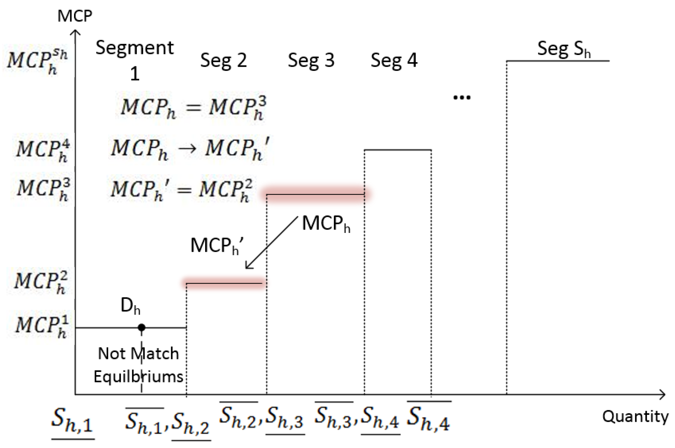
In this part, our proposed new algorithm will be illustrated. From the Equation (2), we know that customers’ demand for hour h can be affected by the price of this hour and other hours. As demonstrated in [14], self-elasticity is usually greater than , we consider the self-elasticity to be the main factor affecting the demand of all customers in this paper. For hour h, if is less (greater) than 0 that means the retail market expects less (greater) electricity demand from the supply side (see second (third) condition in Equation (7)) due to the lower (higher) MCP. In order to reach the match equilibrium in that hour, should be decreased (increased) in order to increase (reduce) the demand. Figure 5 illustrates this scenario: under an MCP vector: , where equals to , i.e., equals to the value of third segment in hour h’s MCP function (as can be seen in Equation (1)), the total customers’ demand is not located within the same segment as with a less amount, which means that the match equilibrium in hour is not reached. As a result, should be decreased to where equals to to increase the demand in order to decrease the value of and to reach the match equilibrium in that hour. We can use the same idea to find the match equilibria for the remaining hours. Based on the above example, we propose a formal Algorithm 2 to attain the match equilibriums for H hours of next day. Note that Algorithm 2 is the ultimate solution algorithm for the whole integration problem.
| Algorithm 2 Analytical optimization method | |
| Input:MCP function of each hour (Table 1); A random MCP vector generating from Table 1. | |
| Output: A MCP vector (which reaches the match equilibriums); | |
| 1: | Retailers calculate problem (5) by using the input MCP vector; |
| 2: | The ISO calculates for each hour and gets a vector: Er = ; |
| 3: | While exists ; |
| 4: | Find hour h in the set of , where ; |
| 5: | If & ; |
| 6: | Decreases to the value of previous segment in Table 1; |
| 7: | If ; |
| 8: | Increases to the value of next segment in Table 1; |
| 9: | Retailers calculate problem (5) under the modified new MCP vector and get new for each hour; |
| 10: | End while; |
| 11: | Output the final MCP vector and each retailer’s estimated demand. |
In order to ensure the correctness and feasibility of this new algorithm in our mechanism, it is necessary to prove the monotonicity in step 3. If we can prove that the property of monotonicity is held in step 3, this means that will be decreased after each loop. Then we can say that our algorithm becomes closer to the final result (find a MCP vector which makes ) after each loop. Besides, we should also prove the convergence of Algorithm 2. If we can prove that property, which means Algorithm 2 can converge (i.e., find a MCP vector which makes ) after limited numbers of iterations, we can say that our algorithm is feasible to the proposed mechanism.
Firstly, we define the monotonicity of our algorithm:
Definition 2.
For hour h, we have(or) andwhere) (or)), then change the value offromto(or), we useto present the changed . If Equation (9) holds, we can say that each iteration in step 3 is monotone.
In Equation (9), mean all hours in H except for hour h, . For the scenario of and (or and ), cannot be increased (or decreased), which is the reason that we set ) (or )). It means that the preferred customers’ demand in that hour violates the given demand interval from the ISO. When this happens, the match equilibrium may not be reached. Such situations should be avoided by the ISO. A simple solution is to make sure the declared hourly demand interval be wide enough to consider all possible demand from the retail market.
To facilitate the understanding and for the purpose of illustration, we set H equal to 2 and j equal to 1 (that is only two time periods and one retailer are considered) in our proof process. However, the proof is also applicable to cases where there are more than one retailer and more time periods. For the case of the number of retailers, this is mainly because the cross effects of customers among different retailers can be ignored in the context of day-ahead dynamic pricing in the retail market. For the case of time periods, since in each loop of Algorithm 2 we only change a single hour’s MCP ( changes to ) and in the proof process we split into two parts: and (i.e., all other hours except h as a whole) considering how the change in affects these two parts separately, there is no difference when H is set to be 2 or other values, e.g., 24. Based on the above analysis, the setting of these two parameters (i.e., number of retailers and time periods) does not affect the correctness of our proof process. As a result, in the following proof process, we consider H = 2 (i.e., the peak hour and off-peak hour) and j = 1 (one retailer) without loss of generality. Given the demand functions of the retailer in both time periods represented in Equations (10)–(12):
the optimization problem in Equation (5) can be written to Equations (13)–(15):
In our proof process, we will use two theorems. In the following we will prove these two theorems firstly before we present the proof of monotonicity and convergence of Algorithm 2.
Theorem 1.
In problem (13), we assume that the retailer’s optimal retail price in the peak hour will stay the same or decrease (increase) when is decreased (increased).
Proof.
The optimal point of has three different scenarios when is unchanged. Since the Equation (13) is a quadratic equation and the decision variables are and , we can plot it as a parabola in the coordinate system. The x axis represents the value of and y axis represents the value of . The first scenario is that the optimal solution is in the peak point of Equation (13)’s parabola when the peak point is satisfied the constraints in Equations (14) and (15). On the contrary, the optimal solution is not the peak point in the parabola in both the second and third scenario: the optimal is in the boundary of constraint in Equations (14) and (15) respectively. The Equation (13) can be transferred to:
☐
According to the peak-point equation in the quadratic equation, we know for equation , the peak point is . Based on the differential of Equation (16) of , the value of peak point in x axis is:
From Equation (17), we know is decreased when is decreased. As a result, in the first scenario, we can deduce that will be decreased when is decreased.
In the second scenario, the optimal result of Equation (13) is located at the boundary of sales price constraint Equation (15), which means is equal to (when ) or (when ). We know is decreased when is decreased, which means the parabola of Equation (16) is moved to the left in the coordinate system. Therefore will stay the same when is decreased.
Now we consider the third scenario, the optimal result of (13) is in the boundary of the revenue constraint (14). Then the optimal solution must satisfy the Equation (18):
This equation is also a quadratic equation for . We know for equation , the solution is . Therefore, we can obtain the solution of Equation (18): and , where . In that scenario, the following inequality must be held; otherwise the optimal result of Equation (13) is not located in the boundary of revenue constraint.
The solution space of in that scenario is: and . The optimal is either or . As a result, when Equation (16)’s parabola is moved to the left in the coordinate system, the optimal is either decreased from to or kept the same as before.
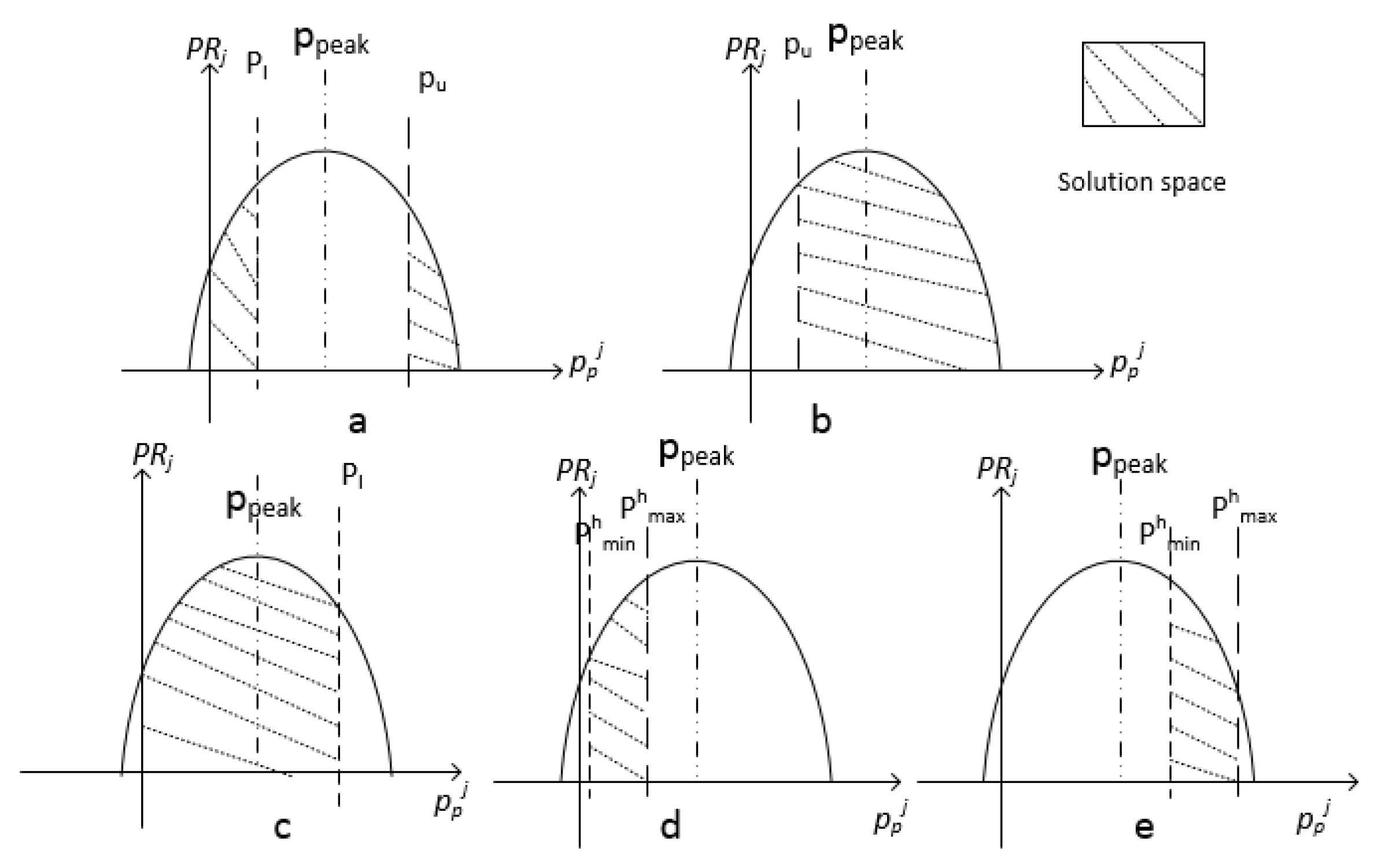
Therefore, we complete the proof of Theorem 1. Figure 6 illustrates the solution space of these three scenarios of problem Equation (13): part (b) and (c) represents scenario 1; part (a) represents scenario 3 and part d and e represent scenario 2.
The second theorem that we used in our proof process is illustrated as follows:
Theorem 2.
The necessary and sufficient condition that the electricity is a demand consistent product in the considered retail market is that, for each , the following inequality holds:
The proof of the above theorem is given in [14]. In the following, we give the proof of the monotonicity and convergence properties in Algorithm 2 (Theorem 3).
Theorem 3.
The monotonicity and convergence properties are held in Algorithm 2. In other words, Algorithm 2 can arrive at the final result (find a MCP vector: , which makes ) after a limited number of iterations.
Proof.
Monotonicity: for peak hour, if is smaller than 0, the retailer’s demand is smaller than the lower bound of corresponding segment in Table 1. According to our new algorithm, the ISO decreases to the value of the previous segment in the MCP table (Table 1) (for example, if , is the second value of column h in Table 1, then decreases from to ), we use to represent the changed . According to Theorem 1, the retailer decreases or keeps unit sales price in the peak hour from to when the unit cost (MCP) in the peak hour from the supply side is decreased. According to Table 1, we can get the Equation (21) when is decreased to :
☐
According to Equations (7) and (8), we calculate the change of after is deceased to:
According to the property of self-elasticity, the demand will increase or keep the same when the retail price in the peak hour is decreased from to , then we can get:
There could be two different situations for , either be bigger than 0 or smaller than 0.
If then:
If :
From (12) and Theorem 2 we know and , so we can conduct that in both of these two situations.
Therefore, we proved the monotonicity in this scenario. Similarly, we can use the same method to prove the monotonicity when is greater than 0. In addition to proving the monotonicity of Algorithm 2, we should also prove the convergence in Algorithm 2 to ensure that the program will finally stop at the point that Er is equal to 0.
Convergence: We set equal to the value of minimum segment in the Table 1. From Equations (24)–(26), we know that:
Assuming is the result of Step 2 in Algorithm 2 and , t is the looping times of step 3 in the algorithm. From Equation (27) we know that:
If Algorithm 2 will never stop, which means . According to Equation (28) we can deduce that:
From the Equation (8) we know . But Equation (29) is contradictory with the condition . Therefore, we can deduce that our algorithm can stop in finite steps, which completes the proof of convergence in the Algorithm 2.
After proofing the convergence and monotonicity, we can say that the using Algorithm 2 in our proposed mechanism can converge to a result that all hours in H can be matched. Then Theorem 3 is proved. The running time T of Algorithm 2 can be given as:
where the above equation indicates that the ISO only calculates optimization problem in Equation (5) for no more than times in proposed mechanism. In the above, is the greatest number in the vector () and t is the running time used for solving the problem in Equation (5) once. It is worth highlighting that the derivation of the upper bound of the running time of Algorithm 2 in Equation (30) is important since it provides meaningful metrics and benchmarks in practical applications and implementation.
5.3. Cases of Renewable Energy Integration
In our proposed approach, given the interval demand provided by the ISO, each generator decides a piecewise constant supply function, which provides a much more flexible scheme than the current one supply volume with one offer price from each generator. For example, in a given hour of the next day, assume that a generation company has three types of power generations: A renewable power supply as type 1 which can generate K1 (kw) electricity with unit cost c1, another renewable power supply as type 2 which can generate K2 (kw) electricity with unit cost c2, and a conventional power supply as type 3 which can generate K3 (kw) electricity with unit cost c3. Then the power supply function is: for the first K1 (kw) supply, the offering price from the generator is (here is the unit profit margin decided by the generator). For the next K2 (kw) supply, the offering price is ; For the further K3 (kw) supply, the offering price is . If the generator knows that there is a lot of renewable supply in type 1 (or type 2 or both) in a given hour or time period next day, then he can reduce unit margin m1, which will lead to a cheaper offer or supply price and as a consequence a cheaper retail price. As a result, it will in turn provide the more incentive to customers for more usages with the cheaper energy (based on the flexibility from the consumers’ side) and lead to higher demand. In this approach, the generated renewable energy will be used up (if price offered or profit margin is set lower enough) or at least used more (if the price offered is not low enough), and the other conventional energy usages in the give hour and/or other hours will be reduced due to the provided incentive. In other words, by tuning the unit profit margin and set the right offer price dependent on the variations of the renewable power availability, the generators have the flexibility to provide a stronger or weaker incentive to the retail markets and in turn to the end customers by offering the right price.
Further the proposed scheme also provides a simpler pricing mechanism as the cost and price can be set based on the individual energy resources and corresponding generation costs rather than a mixed one based on the current mechanism. In other words, this simple example illustrates that the proposed new mechanism provides the generators with the flexibility to integrate the renewable and conventional power resources with one unified framework and enables a simpler pricing mechanism for energy supplying and demand management.
6. Numerical Results
In this section, we present some experiment results. Firstly, the exact parameters are illustrated. All the data are represented in the demand model derived from PJM which includes the day-ahead pricing and demand information between 1 January 2011 and 30 November 2012 [10,28]. Table 2 is the MCP function obtained from the aggregated bidding curve. In order to simplify the calculation, the MCP functions of each hour are set to be the same in the experiment. The constraints in the pricing model are listed as follows: revenue restriction is 34,347,000 $ and max price is 68.398 $/MWh. We consider one retailer in the retail market in the simulation.
In our previous work, we have designed a Genetic Algorithm-based approach to solve the integration problem [26], which is also implemented in this paper based on the above input data and acts as a benchmark algorithm for comparison with our analytical optimization-based solution method. In the following, the process of the GA based approach is described in the context of our considered integration problem.
In genetic algorithm, a population of candidate solutions to an optimization problem has evolved towards finding better solutions. Each candidate solution has a set of properties which can be mutated and altered. In our problem, each combination of MCP vector in MCP table (Table 1) is a candidate solution. The candidate solution has 24 properties which means that each hour is a property; the value of can be mutated and altered. The evolution of the GA algorithm usually starts from a population of randomly generated individuals, and it is an iterative process. A generation in GA means the population in each iteration. In each generation, though solving the objective function in the optimization problem, the fitness value of every individual in the population can be evaluated. The more fit individuals are stochastically selected from the current population, and each individual’s genome is modified (recombined and possibly randomly mutated) to form a new generation. The new generation of candidate solutions is then used in the next iteration of the algorithm. Normally, the algorithm terminates when either a maximum number of generations has been produced, or a satisfactory fitness level has been reached for the population [29,30,31,32]. As we said before, each combination of MCP vector in MCP table is a candidate solution. So the solution domain in our problem is the MCP vector of next 24 h: , in which for any hour . The input of the GA program in our problem is the MCP for the next 24 h. For each MCP vector, the program returns a fitness value according to fitness function which is shown as Equations (7) and (8) (the only difference is that we use and Z rather than and to represent the fitness value in GA). The GA can find the best MCP vector among all combinations of MCP vector which has the best fitness value in certain populations and generations. The program is set to stop when the fitness value is less than 2% of yesterday’s demand or a fixed number of generations are reached, whichever become first.
Analysis of the Results
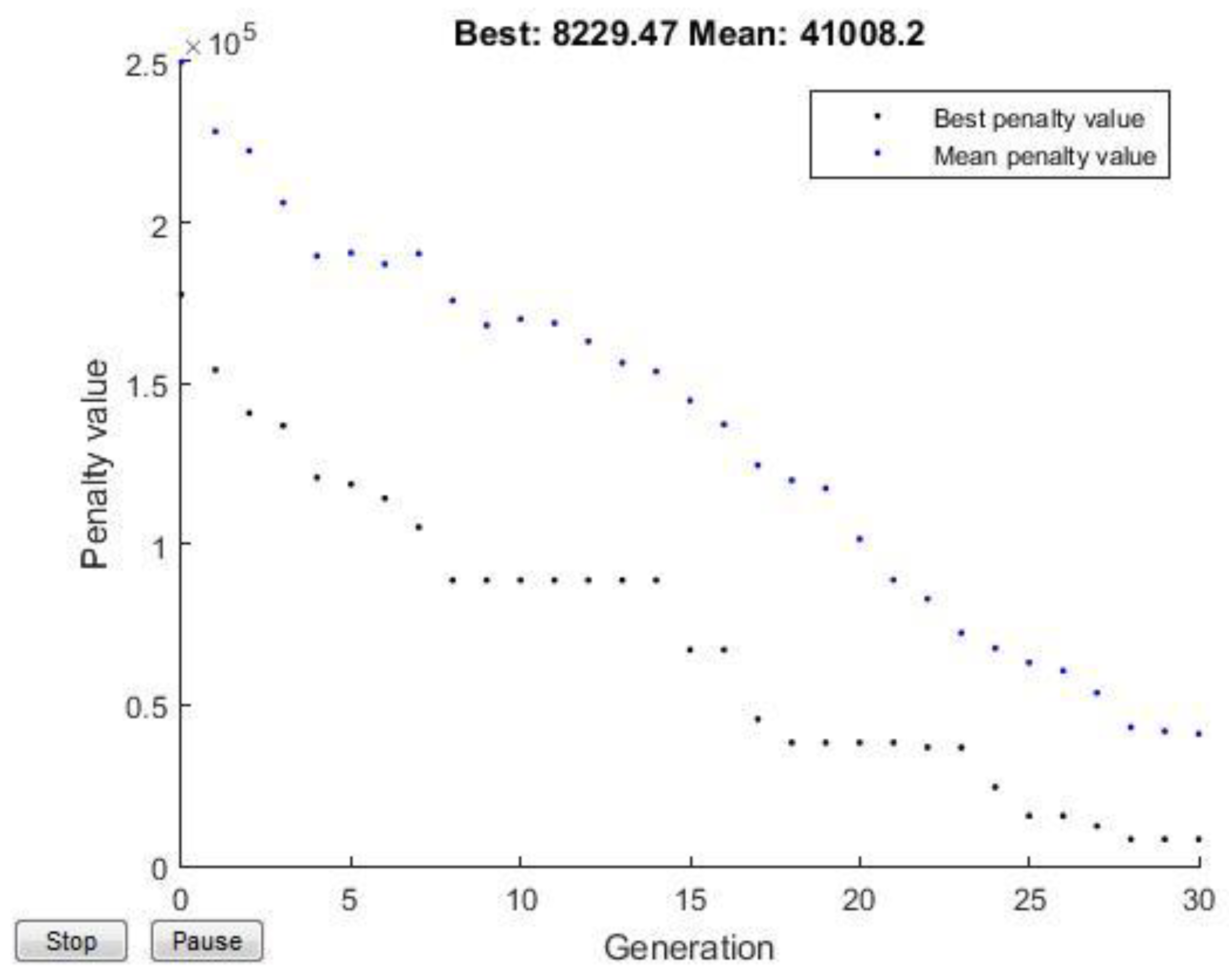
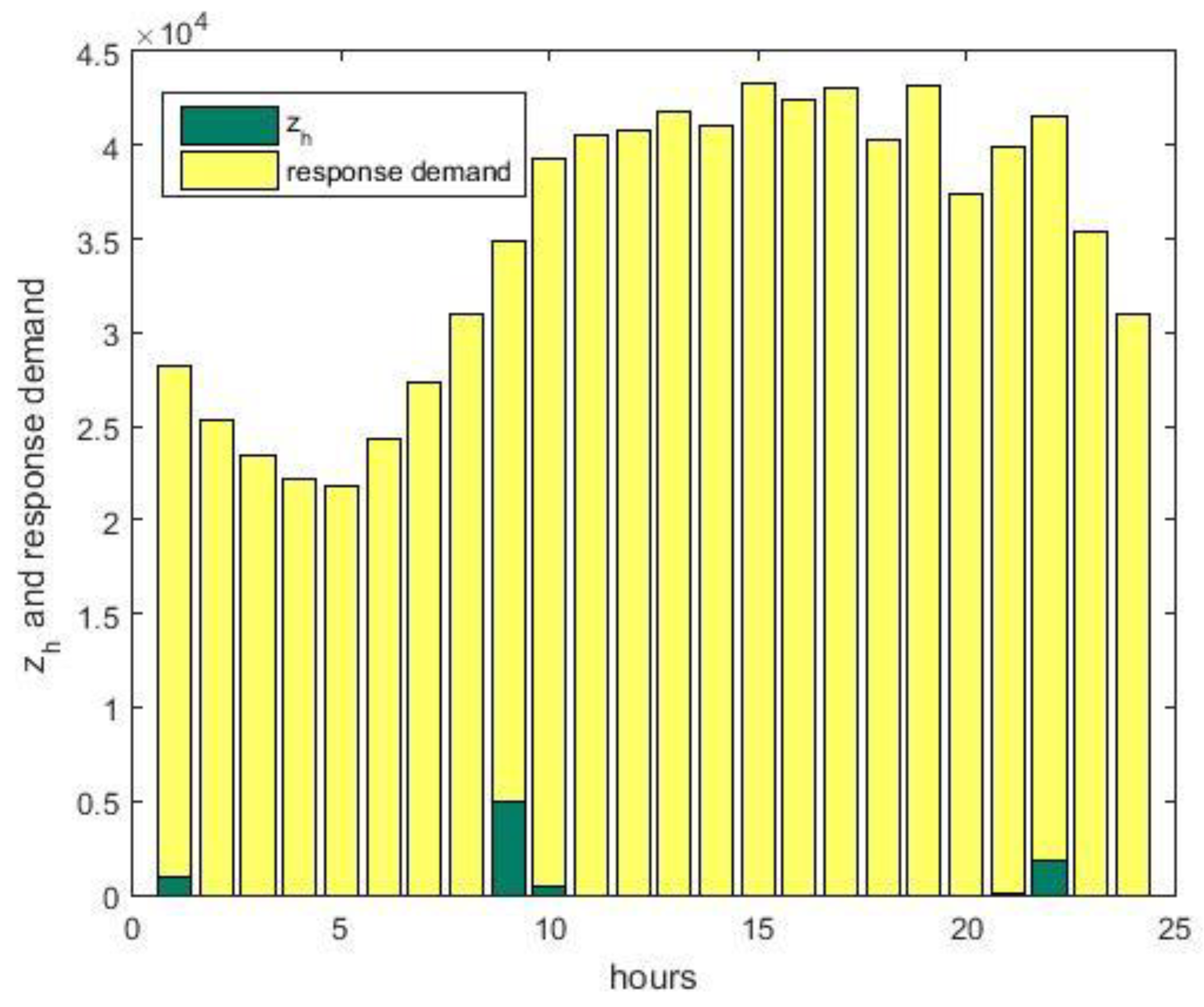
Figure 7 is the running result of the Genetic Algorithm under the MCP function shown in Table 2. The max generation is set as 30 and the match threshold value is set as 2% of yesterday’s demand: 16,786.56 MWh. After 28 generations, the best objective value (i.e., ) of GA method is 8229.47 MWh, which is quite a small number compared with the average demand per hour from all customers: 34,972 MWh. Table 3 show the details of the best fitness value () under the final MCP vector in 24 h. It can be found that in most hours equals zero, which means that the total customers’ demand in hour h is located within the supply segment: in Table 1. Figure 8 present the hourly demand from customers and the fitness value in each corresponding hour under the final MCP vector. It can be found that there are 5 h where is not equal to 0, which account for 3.26%, 14.23%, 1.18%, 0.31% and 4.24% respectively of the corresponding demand in each of those hours.
As aforementioned, it is not possible to find an exact mathematical optimization problem to solve the integration problem directly. As there are many possible combinations of MCP vectors, it is not tractable to use enumeration method to solve the problem. For instance, for small cases where only 10 hours’ MCP are considered varying and the corresponding MCP function of each hour takes only two segments in Table 2, it requires to solve the retailer’s smart pricing problem for times and takes around 3 h to finish for enumeration method. Image that if we only consider two MCP function segments but for each of those 24 h (i.e., all 24 hours’ MCP are considered varying), this is still a relatively small case but already gives us a solution space of possible MCP vectors. In other words, we need to solve Equation (5) for times in this case for the enumeration method, which is obviously intractable and would take months to complete even with a modern cluster. As a result, we developed this GA based metaheuristic algorithm to solve the problem to an approximated solution. Although from the above results, GA could give a reasonable solution, the limitations of such algorithm are also obvious: for GA based solution method, it still needs to solve the retailer’s pricing optimization problem for many times due to its iteration nature and can only solve the problem to an approximated solution (e.g., as can be seen from the above among 24 h, the match equilibriums for 5 h are not attained under GA based method). Although a better result could be obtained e.g., by increasing the number of generation, the running time of GA-based method will increase dramatically and suffer from the scalability issues.
For the above considered example, under the environment of 8 GB RAM, 3.20 GHz Intel Core processor with parallel processing, GA-based method needs 10 h to obtain the above result when the max generation is set as 30 and the population size as 60. Therefore, (1) the GA based method in this case might work for small problem size but would suffer from scalability issues when the problem size grows; (2) the implementation of GA based method requires each retailer to determine the optimal price for so many times (1800 times in our experiment), thus requiring huge information exchanges/communication between the ISO and retailers frequently. These limitations are overcome by our Analytical optimization method.
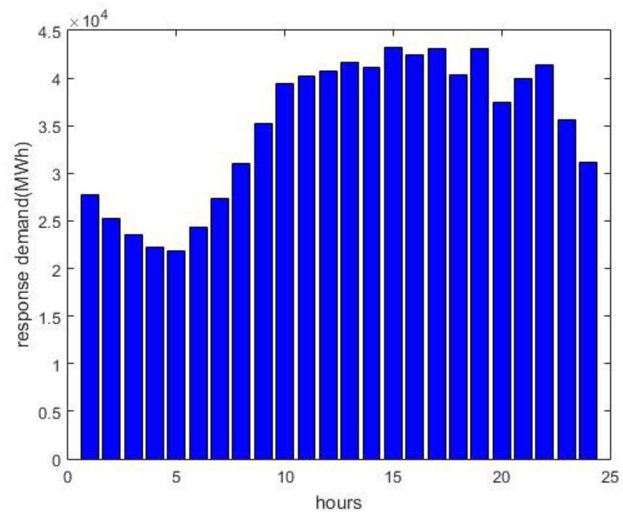
For our Analytical optimization method, after only a few numbers of iterations, the objective value of in our experiment becomes 0. The running result of Algorithm 2 under the MCP function is showed in Table 4. It can be found that equals to zero for each hour, which means the customers’ reaction demand for hour h is in the same segment with the MCP of that hour. It also means the ISO finds the match equilibrium in all hours of the next day. In contrast to the long running time of GA-based method (which takes about 10 h), the running time of Algorithm 2 is only for about 15–45 min, showing that our new method is much more efficient and accurate than GA based method. In addition, Figure 9 shows the customers’ demand (estimated reaction demand) under the final/optimal MCP. From the above results, it can be found that the proposed integration mechanism and the analytical optimization-based solution algorithm are feasible and effective.
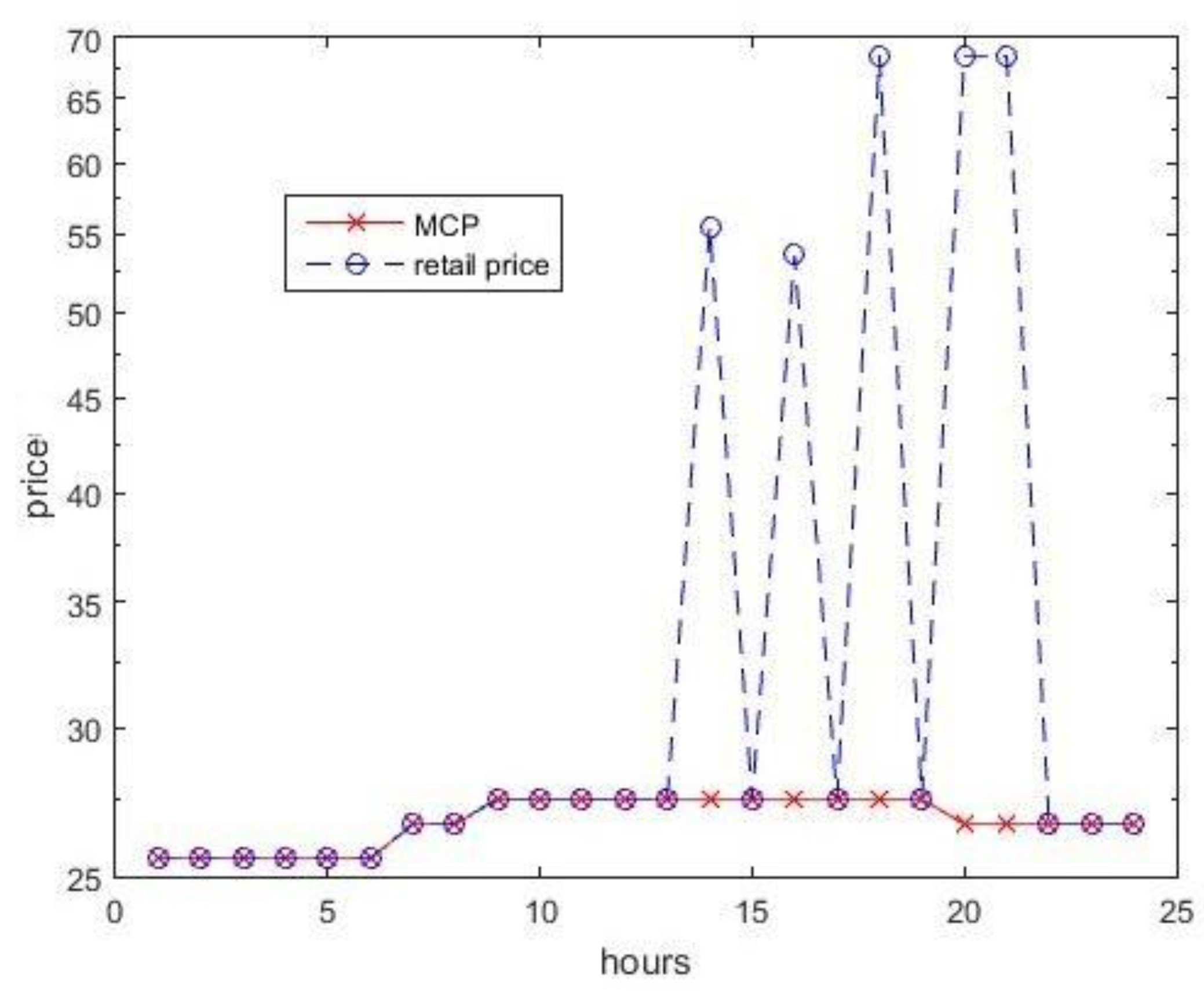
The detailed results of the dynamic pricing model of the retailer in the retail market within the analytical optimization method are also given in the following. Firstly, the retailer’s revenue in this the experiment under the final MCP is 29,728,216 $, which satisfies the revenue constraint. On the other hand, it indicates that our dynamic pricing model enables the retailer to optimize its profit without increase the revenue. Secondly, Figure 10 shows the comparison between the final MCP vector in the wholesale market and the dynamic retail price of the retailer. It can be found that the retail prices in peak hours are increased compared with the wholesale MCP. This is to encourage customers to reduce their consumption in peak hours and shift their consumption from peak-periods to non-peak periods, which is also the reason why the estimated customers’ demand shows a lower peak-to-average ratio of 1.2637. From Figure 10, we can also see that for off-peak hours, the retailer set the retail prices to be low, same as the wholesale MCP. The reason for this is two-fold: (1) the lower off-peak prices will encourage customers to shift their consumption with the incentives of reducing their bills; (2) the inclusion of revenue constraint that we set in Equation (5) ensures that we will have sufficient number of hours with low prices. If we do not include the revenue constraint, the retailer will usually set the price of the electricity as high as they can in order to achieve more profit/revenue. In addition, this will lead to undesirable situations that the prices in hours with small price elasticities (off-peak hours) are set very close to the upper bounds of the retail price constraint, giving bad price image to customers. Based on the above results and analysis, it demonstrates that our proposed integration mechanism and solution algorithm are efficient in finding the match equilibriums for the demand response integration problem and in enabling the smart pricing strategy of retailers in the retail market.
7. Conclusions
The work in this paper presents an integration mechanism with demand response which integrates the demand-side and supply-side as well as its market counterparts (i.e., retail market and wholesale market). Different from the existing market mechanism, where the ISO only declares a single demand to the generators or suppliers in the wholesale market, in our mechanism the ISO declares a demand interval to the wholesale market for each hour. The demand interval is easy to estimate and more robust than a single demand figure and enables the ISO to handle unpredictable demand under the DR programs in our mechanism. Another important contribution of this paper is to propose an analytical optimization method to find the match equilibrium between the demand and supply side in the new mechanism. A formal proof is also given to prove the feasibility and effectiveness of the proposed analytical optimization solution method. Through a comparative analysis of the simulation results by comparing the proposed analytical optimization-based solution method with a GA-based benchmark solution method, it demonstrates the feasibility and effectiveness of the proposed integration mechanism and analytical optimization-based solution algorithm in enabling the demand response integration and reasonable smart retail pricing strategies. For instance, the proposed analytical solution method can find the matching equilibriums for all considered hours with only around 15–45 min, which is more effective and efficient than the GA-based benchmark solution method (which takes about 10 h to only find an approximated solution).
Although the work of this paper fulfills the aims of developing an effective energy system in order to balance the demand and supply in the Smart Grid, there is still some work that can be developed in the future, such as proposing different pricing models for different types of customers. With the information from the smart meter, the retailer could classify the customers into different types: price-making customers and price-taking customers. Therefore, different pricing strategies can be offered to different customers in order to incentivize them to participate in potential demand response programs. In addition, we plan to investigate the computational aspects of the problem further in our future work including taking advantage of modern distributed and parallel computational facilities in solving very large-scale demand response integration problems.
Author Contributions
X.J.Z. and Z.L. conceived of the presented idea. Z.L. carried out the experiment and analysis the data. Z.L. wrote the manuscript with the support from X.J.Z. and the input from F.M. F.M. revised the manuscript. All authors discuss the reviewers’ comments and contributed to final manuscript.
Funding
This research received no external funding.
Conflicts of Interest
The authors declare no conflicts of interest.
Nomenclature
| Parameter | Description |
| h | h-th hour |
| -th generator | |
| j | j-th retailer |
| The number of segments in this generator i’s bid curve | |
| Bid price of -th segment in generator i’s bid curve | |
| Lower bound of -th segment in generator i’s bid curve | |
| Upper bound of -th segment in generator i’s bid curve | |
| Market clear price in hour h | |
| The number of total segments in all generators’ bidding curves (MCP function) of hour h, where | |
| The k-th segment of the proposed step function (aggregated bidding curve) in hour h | |
| the demand from the retail market in hour h | |
| The corresponding unit price of | |
| The cross-price elasticity | |
| The self-elasticity | |
| The maximum price that the retailer can offer to its customers | |
| The minimum price that the retailer can offer to its customers | |
| The total bill constraint of retailer j’s customers | |
| The retailer j’s optimal retail price in hour h | |
| The total demand of retailer j’s customers in hour h | |
| Fitness value of a MCP vector in hour h (Analytical optimization Method) | |
| Er | Fitness value of a MCP vector (Analytical optimization Method) |
| The MCP vector which makes the electricity market reaches the match equilibrium | |
| Market clearing price for -th segment in hour h under the MCP table (Table 1) | |
| All hours in (1, … H) except for hour h | |
| Retailer j’s demand in hour h. | |
| Retailer j’s profit in period (1, … H). | |
| P | Peak hour |
| o | Off-peak hour |
| Lower bound of ’s corresponding supply in Table 1 | |
| Upper bound of ’s corresponding supply in Table 1 | |
| The value of peak point in x axis for quadratic function. | |
| The biggest number in the vector () |
References
- Fang, X.; Misra, S.; Xue, G.; Yang, D. Smart grid—The new and improved power grid: A. survey. IEEE Commun. Surv. Tutor. 2012, 14, 944–980. [Google Scholar] [CrossRef]
- Blumsack, S.; Fernandez, A. Ready or not, here comes the smart grid! Energy 2012, 37, 61–68. [Google Scholar] [CrossRef]
- Meng, F.L.; Zeng, X.J. A profit maximization approach to demand response management with customers’ behavior learning in smart grid. IEEE Trans. Smart Grid 2016, 7, 1516–1529. [Google Scholar] [CrossRef]
- Kirschen, D.S.; Strbac, G.; Cumperayot, P. Factoring the elasticity of demand in electricity prices. IEEE Trans. Power Syst. 2000, 15, 612–617. [Google Scholar] [CrossRef]
- Mohsenian-Rad, A.H.; Leon-Garcia, A. Optimal residential load control with price prediction in real-time electricity pricing environments. IEEE Trans. Smart Grid 2010, 1, 120–133. [Google Scholar] [CrossRef]
- Su, C.L.; Kirschen, D. Quantifying the effect of demand response on electricity markets. IEEE Trans. Power Syst. 2009, 24, 1199–1207. [Google Scholar] [CrossRef]
- Albadi, M.H.; El-Saadany, E.F. Demand response in electricity markets: An overview. In Proceedings of the Power Engineering Society General Meeting, Tampa, FL, USA, 24–28 June 2007; pp. 1–5. [Google Scholar] [CrossRef]
- Rassenti, S.J.; Smith, V.L.; Wilson, B.J. Controlling market power and price spikes in electricity networks: Demand-side bidding. Proc. Natl. Acad. Sci. USA 2003, 100, 2998–3003. [Google Scholar] [CrossRef] [PubMed] [Green Version]
- Aalami, H.A.; Moghaddam, M.P.; Yousefi, G.R. Modeling and prioritizing demand response programs in power markets. Electr. Power Syst. Res. 2010, 80, 426–435. [Google Scholar] [CrossRef]
- Walawalkar, R.; Fernands, S.; Thakur, N.; Chevva, K.R. Evolution and current status of demand response (DR) in electricity markets: Insights from PJM and NYISO. Energy 2010, 35, 1553–1560. [Google Scholar] [CrossRef]
- Kassakian, J.G.; Schmalensee, R.; Desgroseilliers, G. The Future of the Electric Grid. MIT. Available online: http://web.mit.edu/mitei/research/studies/the-electric-grid-2011.shtml (accessed on 26 March 2017).
- ISO RTO. Available online: http://en.wikipedia.org/wiki/ISO_RTO (accessed on 06 August 2017).
- Ma, Z.; Billanes, J.D.; Jørgensen, B.N. Aggregation potentials for buildings—Business models of demand response and Virtual Power Plants. Energies 2017, 10, 1646. [Google Scholar] [CrossRef]
- Ma, Q.; Zeng, X.J. Demand modelling in electricity market with day-ahead dynamic pricing. In Proceedings of the 2015 IEEE International Conference on Smart Grid Communications (SmartGridComm), Miami, FL, USA, 2–5 November 2015; pp. 97–102. [Google Scholar] [CrossRef]
- Aalami, H.A.; Moghaddam, M.P.; Yousefi, G.R. Demand response modeling considering interruptible/curtailable loads and capacity market programs. Appl. Energy 2010, 87, 243–250. [Google Scholar] [CrossRef]
- Maharjan, S.; Zhu, Q.; Zhang, Y. Dependable demand response management in the smart grid: A Stackelberg game approach. IEEE Trans. Smart Grid 2013, 4, 120–132. [Google Scholar] [CrossRef]
- Bu, S.; Yu, F.R.; Liu, P.X. A game-theoretical decision-making scheme for electricity retailers in the smart grid with demand-side management. In Proceedings of the 2011 IEEE International Conference on Smart Grid Communications (SmartGridComm), Brussels, Belgium, 17–20 October 2011; pp. 387–391. [Google Scholar] [CrossRef]
- Chen, J.; Yang, B.; Guan, X. Optimal demand response scheduling with stackelberg game approach under load uncertainty for smart grid. In Proceedings of the 2012 IEEE Third International Conference on Smart Grid Communications (SmartGridComm), Tainan, Taiwan, 5–8 November 2012; pp. 546–551. [Google Scholar] [CrossRef]
- Faruqui, A.; Hajos, A.; Hledik, R.M. Fostering economic demand response in the Midwest ISO. Energy 2010, 35, 1544–1552. [Google Scholar] [CrossRef]
- Faria, P.; Vale, Z. Demand response in electrical energy supply: An optimal real time pricing approach. Energy 2011, 36, 5374–5384. [Google Scholar] [CrossRef] [Green Version]
- Yu, M.; Hong, S.H. Incentive-based demand response considering hierarchical electricity market: A Stackelberg game approach. Appl. Energy 2017, 203, 267–279. [Google Scholar] [CrossRef]
- Samadi, P.; Mohsenian-Rad, H.; Schober, R. Advanced demand side management for the future smart grid using mechanism design. IEEE Trans. Smart Grid 2012, 3, 1170–1180. [Google Scholar] [CrossRef]
- Mohsenian-Rad, A.H.; Wong VW, S.; Jatskevich, J. Autonomous demand-side management based on game-theoretic energy consumption scheduling for the future smart grid. IEEE Trans. Smart Grid 2010, 1, 320–331. [Google Scholar] [CrossRef]
- Li, C.A.; Svoboda, A.J.; Guan, X. Revenue adequate bidding strategies in competitive electricity markets. IEEE Trans. Power Syst. 1999, 14, 492–497. [Google Scholar] [CrossRef]
- Liu, Z.; Zeng, X.; Yang, Z.-L. Demand Based Bidding Strategies Under Interval Demand for Integrated Demand and Supply Management. In Proceedings of the 2018 IEEE Congress on Evolutionary Computation (CEC), Rio de Janeiro, Brazil, 8–13 July 2018. [Google Scholar] [CrossRef]
- Liu, Z.; Zeng, X.J.; Ma, Q. Integrating demand response into electricity market. In Proceedings of the 2016 IEEE Congress on Evolutionary Computation (CEC), Rio de Janeiro, Brazil, 8–13 July 2018; pp. 2021–2027. [Google Scholar] [CrossRef]
- Yao, L.; Lim, W.; Tiang, S. Demand bidding optimization for an aggregator with a Genetic Algorithm. Energies 2018, 11, 2498. [Google Scholar] [CrossRef]
- PJM. Available online: http://www.pjm.com/ (accessed on 25 July 2014).
- Mitchell, M. An Introduction to Genetic Algorithms; MIT Press: Cambridge, MA, USA, 1998; ISBN 0-262-13316-4. [Google Scholar]
- Goldberg, D.E. Genetic Algorithms in Search, Optimization and Machine Learning; Addison-Wesley Professional: Boston, MA, USA, 1989; ISBN 0201157675. [Google Scholar]
- Reed, P.; Minsker, B.; Goldberg, D.E. Designing a competent simple genetic algorithm for search and optimization. Water Resour. Res. 2000, 36, 3757–3761. [Google Scholar] [CrossRef] [Green Version]
- Genetic Algorithm. Available online: https://en.wikipedia.org/wiki/Genetic_algorithm (accessed on 14 April 2017).
Figure 1.
The structure of electricity market.

Figure 2.
The process of proposed mechanism.

Figure 3.
Example of generators’ bid curve and the aggregated bidding curve. (a) Generator 1’s bid curve; (b) Generator 2’s bid curve; (c) The aggregated bidding curve.
Figure 3.
Example of generators’ bid curve and the aggregated bidding curve. (a) Generator 1’s bid curve; (b) Generator 2’s bid curve; (c) The aggregated bidding curve.

Figure 4.
An example of the match equilibrium.

Figure 5.
An example of the new method.

Figure 6.
The solution space of three scenarios for problem in Equation (13). (a) Scenario 3; (b) Scenario 1(1); (c) Scenario 1(2); (d) Scenario 2(1); (e) Scenario 2(2).
Figure 6.
The solution space of three scenarios for problem in Equation (13). (a) Scenario 3; (b) Scenario 1(1); (c) Scenario 1(2); (d) Scenario 2(1); (e) Scenario 2(2).

Figure 7.
Running result of the GA-based method.

Figure 8.
The customers’ demand and .

Figure 9.
Customers’ demand.

Figure 10.
MCP vector and retailer’s sales price ($/MWH).


Table 1.
The MCP table and corresponding supply segments.
| … | … | ||||
| MCP | Supply Segments | MCP | Supply Segments | ||
| … | … | ||||
| … | … | ||||
| … | … | … | … | … | … |
| … | … | … | … | ||
| … | |||||
| … | |||||
“…” represents the omitted hours’ MCP and corresponded supply segments.
Table 2.
Aggregated bidding curve/MCP function.
| Segment Scale | Segment Number | |||
|---|---|---|---|---|
| 25.5510 | 7100 | 20,200 | 27,300 | 1 |
| 26.6490 | 12,500 | 27,300 | 39,800 | 2 |
| 27.5010 | 8300 | 39,800 | 48,100 | 3 |
| 28.3853 | 8400 | 48,100 | 56,500 | 4 |
| 30.0894 | 7500 | 56,500 | 64,000 | 5 |
| 32.2739 | 9000 | 64,000 | 73,000 | 6 |
| 35.2795 | 7100 | 73,000 | 87,000 | 7 |
| 37.8002 | 12,500 | 87,000 | 91,500 | 8 |
| 42.3322 | 8300 | 91,500 | 98,900 | 9 |
Table 3.
Running results of GA-based method.
| Hour | Hour | Hour | |||
|---|---|---|---|---|---|
| 1 | 920.28 | 9 | 4958.7 | 17 | 0 |
| 2 | 0 | 10 | 463.02 | 18 | 0 |
| 3 | 0 | 11 | 0 | 19 | 0 |
| 4 | 0 | 12 | 0 | 20 | 0 |
| 5 | 0 | 13 | 0 | 21 | 123.434 |
| 6 | 0 | 14 | 0 | 22 | 176.395 |
| 7 | 0 | 15 | 0 | 23 | 0 |
| 8 | 0 | 16 | 0 | 24 | 0 |
Table 4.
Running results of Algorithm 2.
| Hour | Hour | Hour | |||
|---|---|---|---|---|---|
| 1 | 0 | 9 | 0 | 17 | 0 |
| 2 | 0 | 10 | 0 | 18 | 0 |
| 3 | 0 | 11 | 0 | 19 | 0 |
| 4 | 0 | 12 | 0 | 20 | 0 |
| 5 | 0 | 13 | 0 | 21 | 0 |
| 6 | 0 | 14 | 0 | 22 | 0 |
| 7 | 0 | 15 | 0 | 23 | 0 |
| 8 | 0 | 16 | 0 | 24 | 0 |
© 2018 by the authors. Licensee MDPI, Basel, Switzerland. This article is an open access article distributed under the terms and conditions of the Creative Commons Attribution (CC BY) license (http://creativecommons.org/licenses/by/4.0/).
Share and Cite
MDPI and ACS Style
Liu, Z.; Zeng, X.; Meng, F. An Integration Mechanism between Demand and Supply Side Management of Electricity Markets. Energies 2018, 11, 3314. https://doi.org/10.3390/en11123314
AMA Style
Liu Z, Zeng X, Meng F. An Integration Mechanism between Demand and Supply Side Management of Electricity Markets. Energies. 2018; 11(12):3314. https://doi.org/10.3390/en11123314
Chicago/Turabian StyleLiu, Zixu, Xiaojun Zeng, and Fanlin Meng. 2018. "An Integration Mechanism between Demand and Supply Side Management of Electricity Markets" Energies 11, no. 12: 3314. https://doi.org/10.3390/en11123314
Note that from the first issue of 2016, this journal uses article numbers instead of page numbers. See further details here.