Energy Modeling and Parameter Identification of Dual-Motor-Driven Belt Conveyors without Speed Sensors


School of Information and Control Engineering, China University of Mining and Technology, Xuzhou 221116, China
*
Author to whom correspondence should be addressed.
Energies 2018, 11(12), 3313; https://doi.org/10.3390/en11123313
Submission received: 15 October 2018
/
Revised: 22 November 2018
/
Accepted: 23 November 2018
/
Published: 27 November 2018
(This article belongs to the Section I: Energy Fundamentals and Conversion)
Abstract
:The energy model of belt conveyors plays a key role in the energy efficiency optimization problem of belt conveyors. However, the existing energy models and parameter identification methods are mainly limited to single-motor-driven belt conveyors and require speed sensors. This paper will present an energy model and a parameter identification method for dual-motor-driven belt conveyors whose speed sensors are not available. Firstly, a new energy model of dual-motor-driven belt conveyors is established by combining the traditional energy model with the dynamic model of a dual-motor-driven system. Then, a parameter identification method based on an extended Kalman filtering algorithm and recursive least square approach is proposed. Finally, the feasibility and effectiveness of the method are demonstrated by simulation experiments.
1. Introduction
Belt conveyors play an important role in continuous bulk material transport in the mining industry, chemical production, power plants, and so on [1,2]. As shown in Figure 1, a belt conveyor is mainly composed of a belt, drive motor, drive pulley, roller, and take-up device [1]. The drive pulley is powered to rotate the belt and move the materials on the belt forward [2]. The traditional control for belt conveyors can only make belt conveyors run at a constant speed [2,3], and the average utilization of a belt is less than the design capacity [4], which may lead to a large amount of energy wastage. According to standard DIN 22101, considerable energy savings can be achieved by adjusting the belt speed in accordance with a change in material feed rate [5]. However, the relationship among the energy consumption, feed rate, and belt speed is complex, and the energy consumption is also closely related to the working environment and the operational condition of the drive motors [6]. Therefore, it is of great importance to study the energy model and parameter identification methods for belt conveyors, which have been concerns for many scholars [7,8,9,10].
The existing energy models of belt conveyors can be mainly divided into two categories: data-driven energy models [11,12] and analytical energy models [7,13,14,15,16]. The accuracy of data-driven energy models is affected by experimental data greatly. Thus these models are not conducive to formulate and solve the EEO (energy efficiency optimization) problems. For EEO problems, analytical energy models are more reasonable.
The classical analytical energy models originated from ISO 5048, DIN 22101 and CEMA (Conveyor Equipment Manufacturers Association) are based on resistance calculation. But they involve too many parameters and can hardly be used for EEO problems. According to JIS B 8805 and FDA (Fenner Dunlop Australia), an alternative analytical energy model is established by energy conversion methodology. This energy model uses fewer parameters but usually results in large errors. Combining with the advantages of the above two methods, an energy model which can be expressed as (1) was established in [6].
where , , and are determined by the structural parameters and operation parameters of the belt conveyors. is the mechanical power of the belt conveyors (kW), is the belt speed (m/s), and is the feed rate (t/h). In practice, many reasons probably make a belt conveyor different to its design condition. Hence, , , , and should be identified through experiments instead of being derived from design parameters [17]. However, is difficult to measure directly, which poses a challenge to the parameter identification of the energy model (1). Based on the relationship among the power and the efficiency of the drive motor and the mechanical power of the belt conveyor, an offline parameter identification method based on least square and an online parameter identification method based on recursive least square were proposed in [17]. However, for a dual-motor-driven belt conveyor, the relationship between the efficiency and the mechanical power of the belt conveyor cannot be determined directly. Therefore, the above parameter identification methods cannot be extended to dual-motor-driven belt conveyors directly. An alternative method was proposed by [14], where an energy model was established by combining the energy model with a dynamic model of the drive motor, and a parameter identification method was proposed based on an adaptive observer. In [18], an energy model of belt conveyors driven by rigidly connected dual motors was established by connecting the dynamic model of the drive motors with the energy model of belt conveyors. Meanwhile, a parameter identification method based on recursive least square was proposed. However, drive motors must be equipped with speed sensors in this method. In practice, however, the drive motors may not be equipped with speed sensors and the reasons are as follows: Firstly, speed sensors will increase the size and cost of systems unnecessarily [19]. Furthermore, the reliability of the motors will be influenced [20]. Secondly, the working environment of the drive motors is complex and harsh, so the speed sensors are prone to failure and their maintenance is very difficult. Thirdly, it is also not suitable for installing speed sensors in hostile environments [21]. Additionally, in some extreme cases, there is no place for installing speed sensors. Furthermore, the speed sensor hinders the development of the motor to achieve a higher speed and miniaturized direction [22,23]. Therefore, this paper will study the problems of energy modeling and parameter identification of dual-motor-driven belt conveyors without speed sensors. The contributions of this paper are as follows: (1) a new energy model of dual-motor-driven belt conveyors is established by combining the classical energy model and the dynamic model of the dual-motor-driven system; (2) a parameter identification method for dual-motor-driven belt conveyors without speed sensors is proposed based on the extended Kalman filtering algorithm and recursive least square. The flowchart of the research is shown in Figure 2.
The rest of this paper is organized as follows: In Section 2, the energy model of belt conveyors based on the dynamic model of the dual-motor-driven system is established. In Section 3, the state observer of the two drive motors is established. EKF (extended Kalman filtering) is adopted to realize the simultaneous estimation of the speed and load torque. Then, a parameter identification method based on RLS (recursive least square) is proposed. In Section 4, simulation results are presented. The last section concludes the paper.
2. Energy Model
This section will establish a new energy model for dual-motor-driven belt conveyors. To do this, the dynamic model of the dual-motor system will be discussed first. Consider that the drive pulley of belt conveyors is driven by two squirrel cage asynchronous motors rigidly connected by a gear transmission system, as shown in Figure 3.
The motion equation of the gear transmission system can be expressed as follows [24]
where is the torque of girth gear, is the friction coefficient of girth gear, is the angular velocity of girth gear, is the load torque and is the load rotating inertia.
The motion equation of the motor is [25]
where is the electromagnetic torque, is the friction coefficient of motor and is the number of pole-pairs. The angular velocity of two motors and the angular velocity of the girth gear meet the following relation.
where is the radius of girth gear, r is the radius of pinion and n is the gearbox reduction ratio.
The motion equation of dual-motor-driven system can be expressed as follows [24]
Then according to (4), we have
Then we have,
where
Because the motors are rigidly connected by gear transmission system, we use to express the speeds of two motors. We use to express the number of pole-pairs. Simplifying (7), yields
In accordance with Flux Orientation Control strategy, the mathematical model of an asynchronous motor oriented by rotor flux can be expressed as follows [25]
where is the mutual induction, is the self-induction of the rotor, and is the self-induction of the stator; and are the components of the stator currents, respectively; is the stator phase resistance and is the rotor phase resistance; is the rotor flux; and are the components of stator voltages, respectively; is the coefficient of the leakage inductance which is determined by ; is the rotor time constant which is determined by ; is the synchronous speed and it is accurately calculated using .
The first equation of (10) is the motion equation of motor, and the load is assumed to be a slowly time-varying value, then the torsional elastic torque and damping torque can be ignored. Hence, the electromagnetic torque can be expressed as follows
In accordance with Flux Orientation Control strategy, the stator current is decomposed into excitation current and torque current. The rotor flux produced only by excitation current, and the electromagnetic torque is proportional to the product of rotor flux and torque current. Hence, the components between torque and magnetic field of stator current are decoupled.
Therefore, the dynamic model of dual-motor-driven system is given by
where is time constant and can be expressed as
For a belt conveyor, the load torque can be expressed as follows
where is the total resistance of the belt conveyors, is the radius of the drive pulley.
According to [6], the total resistance of the belt conveyors can be calculated by
The belt speed can be accurately calculated by , and . is the bulk density of material () and is the width between the skirt boards (m). is the artificial friction factor. is the center-to-center distance (m). is a constant. is the mass of the moving parts of the equipment (); it can be expressed as . is the unit mass of the rotating parts of the carrying idler rollers (), is the unit mass of the rotating parts of the return idler rollers (), and is the unit mass of the belt (). , , and are the constants which relate to the structural parameters of the belt conveyor.
Combining (14) and (15), we have
where
Then incorporating into according to (9) and (16), we have
As a result, the energy model of dual-motor-driven belt conveyors can be expressed as follows
The advantage of this energy model is that the dynamic model of the dual-motor-driven system is involved, which is convenient for parameter identification. The model proposed in this section can be used for an energy model of dual-motor-driven belt conveyors.
The vector is determined by the structural parameters of the belt conveyor, which are difficult to measure. Hence is the parameter to be identified.
Remark 1.
The energy model of dual-motor-driven belt conveyors is established by combing the classical energy model (1) with the dynamic model of the dual-motor-driven system (12). Compared with the data-driven energy model in [11], the proposed model (20) is more convenient to formulate the energy optimization problem of belt conveyors. From the view point of parameter identification, the proposed model (20) is applicable to dual-motor-driven belt conveyors, while the analytical energy model in [14] and [17] can only be applied to single-motor-driven belt conveyors.
3. Parameter Identification
In this section, a new parameter identification method will be proposed for the energy model of dual-motor-driven belt conveyors without speed sensors. The basic idea is as follows: firstly, the linearized state space model of the system will be established. Then, the EKF algorithm is used to estimate the speed and total load torque of the belt conveyors [26,27,28]. Finally, the RLS algorithm is adopted to identify the energy model parameters. The scheme of identification is shown in Figure 4.
3.1. State Space Model of the Energy Model
The energy model (20) can be rewritten as follows
We rewrite (21) as
where is the differential operator. In the process of implementing the EKF algorithm, the continuous system needs to be discretized. Equation (22) can be expressed as follows
where is the sampling time, the recurrence formula of matrix can be obtained by combining (22) and (23) as follows
where
with , , . The state variables are denoted as follows
Then, we have
where is the interference and is the measurement noise caused by inaccurate measurement. In general, and are assumed to be Gaussian white noise with zero mean.
3.2. Extended State Equation of the Energy Model
Selecting and as state variables, the extended state equation of the energy model (27) is as follows
where is the extended state matrix which can be expressed as
Equation (29) can be rewritten as follows
Then, we have
A linearized model of (32) will be used in the sequel. So we define and as follows
Combining (32) and (34), we have
Furthermore,
where .
Then combining (29)–(36), the extended discrete state space model is established as follows
where and are the covariance matrix of and , respectively.
3.3. Parameter Identification of the Energy Model Based on EKF and RLS
Based on (37), EKF can be used to estimate and . The scheme of EFK is shown in Figure 5.
The steps of EKF algorithm are as follows
- Prediction of state:where is the estimated state at , is the predicted state at .
- Estimation of error covariance matrix:where is the state error covariance at . is the predicted state error covariance. is the assumed process noise covariance.
- Computation of the Kalman filter gain:
- State Estimation:where is the output measurement of system at , is the predicted Jacobian matrix at .
- Update of the error covariance matrix:
The relationship among the motor speed, material feed rate, load torque and the parameters of energy model can be expressed as follows
Combining (20) and (43), we have
Because speed and load torque of the dual-motor-driven system can be estimated by EKF algorithm. So we define
Therefore, combining with the estimated results, the basic form of least square method for the energy model of the dual-motor-driven belt conveyors can be written as follows
In order to avoid calculating the matrix inversion in the identification process, the recursive least square method is adopted in this paper, the algorithm is implemented by the following equations [29].
Remark 2.
The proposed parameter identification method for the energy model consists of EKF and RLS. EKF is adopted to estimate the motor speed and load torque, and RLS is used to identify the parameters of the energy model base on the estimated value of the motor speed and load torque. Compared with the existing parameter identification methods of energy models [14,17,18], the advantages of this method are as follows: 1) speed sensors are not required; 2) the method is applicable to dual-motor-driven belt conveyors and can be extended to multi-motor-driven belt conveyors.
4. Simulation Study
In this section, the obtained parameter identification method for the energy model of dual-motor-driven belt conveyors without speed sensors will be illustrated. We set the parameters of energy model as , , and [17]. Load is added at 0.04 s, and is set to be as follows [14]
The state vectors of the state observer are as follows
Table 1 gives the parameters of the motors, and sampling time is taken as .
After multiple simulations, the matrices , and are respectively taken as follows
The estimated results of the state variables are given as follows. The EKF algorithm was introduced to estimate and . The estimated speed is displayed in Figure 6, where we can see that the EKF algorithm can estimate the motor speed. The estimated load torque is shown in Figure 7. The figure shows that the estimated load torque can track the time-varying load.
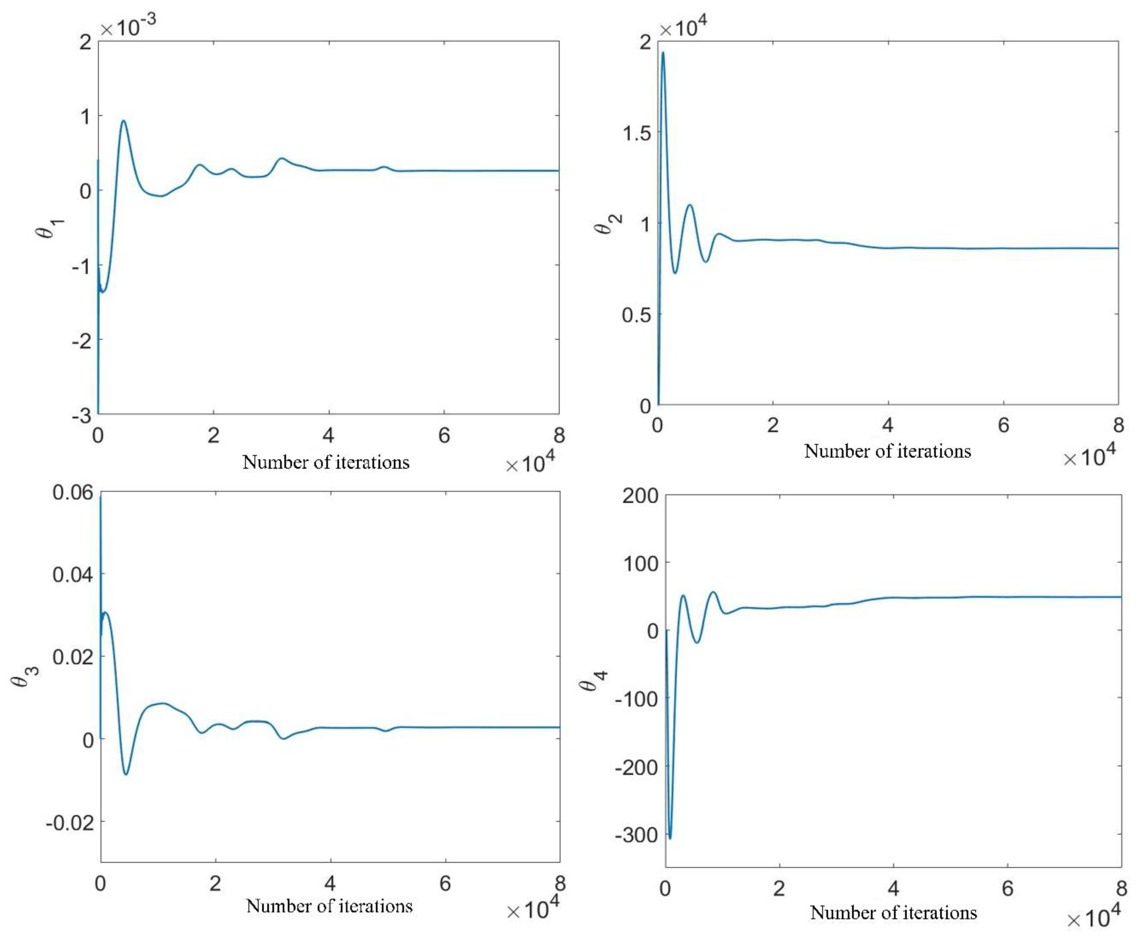
The RLS algorithm is used for identifying the parameters of the energy model, and the results of identification are shown in Figure 8. We can see that the identified values achieve a steady value after approximately 50,000 times recursion, and the identified values of the parameters are obtained. Table 2 shows the comparison between the identified values and the true values. The identification error is less than 4%, and it can be seen that the identified results are acceptable when motor speed and load torque cannot be obtained directly. In the simulation process, the results of the parameter identification based on RLS are influenced by the accuracy of the estimated motor speed and load torque. In addition, the accuracy of the estimated motor speed is greatly influenced by the set values of the EKF algorithm.
5. Discussion
This paper established an energy model and proposed a parameter identification method for dual-motor-driven belt conveyors without speed sensors, which lays a foundation for the energy optimization of belt conveyors. The main contributions are twofold. Firstly, the traditional energy model of belt conveyors is combined with the dynamic model of a dual-motor-driven system to build a new energy model of dual-motor-driven belt conveyors. Secondly, the speed and load torque of the dual-motor-driven system are estimated by using the EKF algorithm to identify the parameters of the energy model. In addition, the identified results of the new parameter identification method are acceptable when the motor speed and load torque cannot be obtained directly.
Based on the electric power of the motor, belt speed, and the feeding rate, a parameter identification method was proposed in [17]. However, this method needs power meters, speed sensors, and electronic belt scales. Furthermore, this method is only applicable to the belt conveyors driven by a single drive motor. So, comparing with the method proposed in [17], the parameter identification method proposed in this paper can be applicable to dual-motor-driven belt conveyors which need not power meters and speed sensors. In [18], based on the measurements of motor current, speed, and feed rate, a parameter identification method is derived by using flux linkage observer and recursive least square. However, drive motors must be equipped with speed sensors in this method. Therefore, the proposed parameter identification method in this paper can compensate for the deficiencies of the above two methods. This means that our method is more applicable in the mining industry, chemical production, power plants, and other complex industrial environments.
The energy modeling method designed in this paper is limited to a rigidly connected gear transmission system. Hence, the energy model of flexible coupling dual-motor-driven belt conveyors needs to be studied in the future. The relationship between the parameters of the energy model and the mechanical parameters of belt conveyors is complex, and the parameters change with the state of belt conveyors. Therefore, it is necessary to design a fast and adaptive method of parameter identification to identify parameters online. Based on the proposed parameter identification method, the energy model of dual-motor-driven belt conveyors without speed sensors can be identified. Thus the relationship among the energy consumption, feed rate, and belt speed will be established. Based on the obtained energy models, the problem of energy optimization of dual-motor-driven belt conveyors can be formulated and studied in the future. The resulted methods can adjust belt speed in accordance with the change in material feed rate to save energy.
Author Contributions
Conceptualization, C.Y.; Data curation, J.L.; Formal analysis, H.L. and L.Z.; Funding acquisition, C.Y.; Investigation, J.L.; Methodology, C.Y.; Project administration, H.L.; Software, J.L.; Supervision, L.Z.; Writing—original draft, J.L. and H.L.; Writing—review & editing, C.Y., H.L. and L.Z.
Funding
This work was supported by the Fundamental Research Funds for the Central Universities under Grant 2017XKQY055.
Acknowledgments
The authors would like to express their gratitude to all those who helped them during the writing of this paper. And the authors would like to thank the reviewers for their valuable comments and suggestions.
Conflicts of Interest
The authors declare no conflict of interest.
References
- Song, W. General Belt Conveyor Design, 1st ed.; China Machine Press: Beijing, China, 2006; pp. 1–2. ISBN 7-111-18415-7. [Google Scholar]
- Pang, Y.S. Intelligent Belt Conveyor Monitoring and Control, 1st ed.; TU Delft: Delft, The Netherlands, 2010; pp. 1–2. ISBN 978–90-5584-134-9. [Google Scholar]
- Ristic, L.B.; Jeftenic, B.I. Implementation of fuzzy control to improve energy efficiency of variable speed bulk material transportation. IEEE Trans. Ind. Electron. 2012, 59, 2959–2969. [Google Scholar] [CrossRef]
- He, D.J.; Pang, Y.S.; Lodewijks, G. Speed control of belt conveyors during transient operation. Powder Technol. 2016, 301, 622–631. [Google Scholar] [CrossRef]
- Hiltermann, J.; Lodewijks, G.; Schott, D. A methodology to predict power savings of troughed belt conveyors by speed control. Part. Sci. Technol. 2011, 29, 14–27. [Google Scholar] [CrossRef]
- Zhang, S.R.; Xia, X.H. A new energy calculation model of belt conveyor. In Proceedings of the IEEE 2009 Green Innovation for African Renaissance, Nairobi, Kenya, 23–25 September 2009. [Google Scholar]
- Mathaba, T.; Xia, X. A parametric energy model for energy management of long belt conveyors. Energies 2015, 8, 13590–13608. [Google Scholar] [CrossRef]
- Marx, D.J.L.; Calmeyer, J.E. A case study of an integrated conveyor belt model for the mining industry. In Proceedings of the 7th Africon Conference in Africa, Gaborone, Botswana, 15–17 September 2004. [Google Scholar]
- Luo, J.; Huang, W.J.; Zhang, S.R. Energy cost optimal operation of belt conveyors using model predictive control methodology. J. Clean. Prod. 2015, 105, 196–205. [Google Scholar] [CrossRef]
- Halepoto, I.A.; Khaskheli, S. Modeling of an integrated energy efficient conveyor system model using belt loading dynamics. Indian J. Sci. Technol. 2016, 9, 47. [Google Scholar] [CrossRef]
- Zhang, Y. Belt Conveyor Energy-Saving Control System Technology Research. Master’s Thesis, Xi’an University of Science and Technology, Xi’an, China, 2014. [Google Scholar]
- Sun, W.; Wang, H.; Yang, H.Q. Research of energy-saving control system with frequency-conversion speed-regulation for belt conveyor. Ind. Mine Autom. 2013, 39, 98–101. [Google Scholar] [CrossRef]
- Xia, X.H.; Zhang, J. Control systems and energy efficiency from the POET perspective. In Proceedings of the IFAC Conference on Control Methodologies and Technology for Energy Efficiency, Vilamoura, Portugal, 29–31 March 2010. [Google Scholar]
- Shen, Y.J.; Xia, X.H. Adaptive parameter estimation for an energy model of belt conveyor with DC motor. Asian J. Control 2014, 16, 1122–1132. [Google Scholar] [CrossRef]
- Middelberg, A.; Zhang, J.; Xia, X. An optimal control model for load shifting—With application in the energy management of a colliery. Appl. Energy 2009, 86, 1266–1273. [Google Scholar] [CrossRef]
- Hiltermann, J.; Lodewijks, G.; Rijsenbrij, J.C. Reducing the power consumption of troughed belt conveyors by speed control. In Proceedings of the 6th International Conference for Conveying and Handling of Particulate Solids, Queensland, Australia, 3–7 August 2009. [Google Scholar]
- Zhang, S.R.; Xia, X.H. Modeling and energy efficiency optimization of belt conveyors. Appl. Energy 2011, 88, 3061–3071. [Google Scholar] [CrossRef] [Green Version]
- Yang, C.Y.; Li, H.; Che, Z.Y. Energy consumption modeling and parameter identification for double-motor driven coal mine belt conveyers. Control Theor. Appl. 2018, 35, 335–341. [Google Scholar] [CrossRef]
- Barut, M.; Bogosyan, S.; Gokasan, M. EKF based sensorless direct torque control of IMs in the low speed range. In Proceedings of the IEEE International Symposium on Industrial Electronics, Dubrovnik, Croatia, 20–23 June 2005. [Google Scholar]
- Maes, J.; Melkebeek, J.A. Speed-sensorless direct torque control of induction motors using an adaptive flux observer. IEEE Trans. Ind. Appl. 2000, 36, 778–785. [Google Scholar] [CrossRef]
- Kubota, K.; Matsuse, K. Speed sensorless field oriented control of induction motor with rotor resistance adaptation. In Proceedings of the Industry Applications Society Meeting, Ontario, TO, Canada, 2–8 October 1993. [Google Scholar]
- Wang, J. Study on the Speed Sensorless Vector Control of PMSM. Master’s Thesis, Huazhong University of Science and Technology, Wuhan, China, 2013. [Google Scholar]
- Barut, M.; Bogosyan, S.; Gokasan, M. Speed-sensorless estimation for induction motors using extended Kalman filters. IEEE Trans. Ind. Electr. 2007, 54, 272–280. [Google Scholar] [CrossRef]
- Christopoulos, G.A.; Safacas, A.N.; Zafiris, A. Energy savings and operation improvement of rotating cement kiln by the implementation of a unique new drive system. IET Electr. Power Appl. 2015, 10, 101–109. [Google Scholar] [CrossRef]
- Ruan, Y.; Chen, B.S. Control Systems of Electric Drives-Motion Control Systems, 4th ed.; China Machine Press: Beijing, China, 2012; pp. 179–180. ISBN 978–7-111-27746-0. [Google Scholar]
- Alsofyani, I.M.; Idris, N.R.N.; Jannati, M. Using NSGA II multiobjective genetic algorithm for EKF-based estimation of speed and electrical torque in AC induction machines. In Proceedings of the Power Engineering and Optimization Conference, Langkawi, Malaysia, 24–25 March 2014. [Google Scholar]
- Barut, M.; Bogosyan, S.; Gokasan, M. Experimental evaluation of braided EKF for sensorless control of induction motors. IEEE Trans. Ind. Electr. 2008, 55, 620–632. [Google Scholar] [CrossRef]
- Liu, Y.; Sun, Z. EKF-based adaptive sensor scheduling for target tracking. In Proceedings of the International Symposium on Information Science and Engineering, Shanghai, China, 20–22 December 2008. [Google Scholar]
- Qiang, M.H.; Zhang, J.E. RLS parameter identification and emulate based on matlab/simulink. Autom. Instrum. 2008, 6, 4–5. [Google Scholar] [CrossRef]
Figure 1.
Belt conveyor assembly.
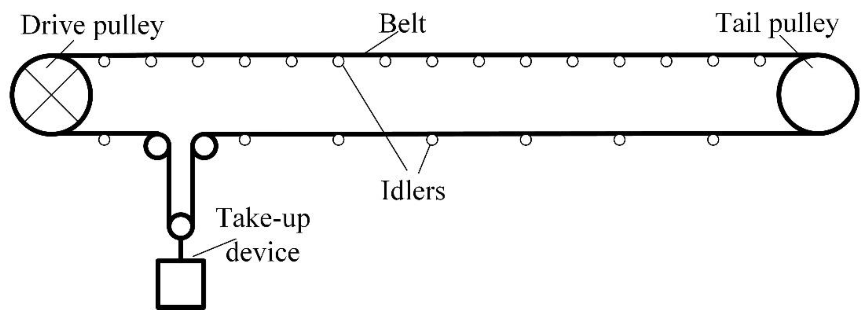
Figure 2.
The flowchart of the research.
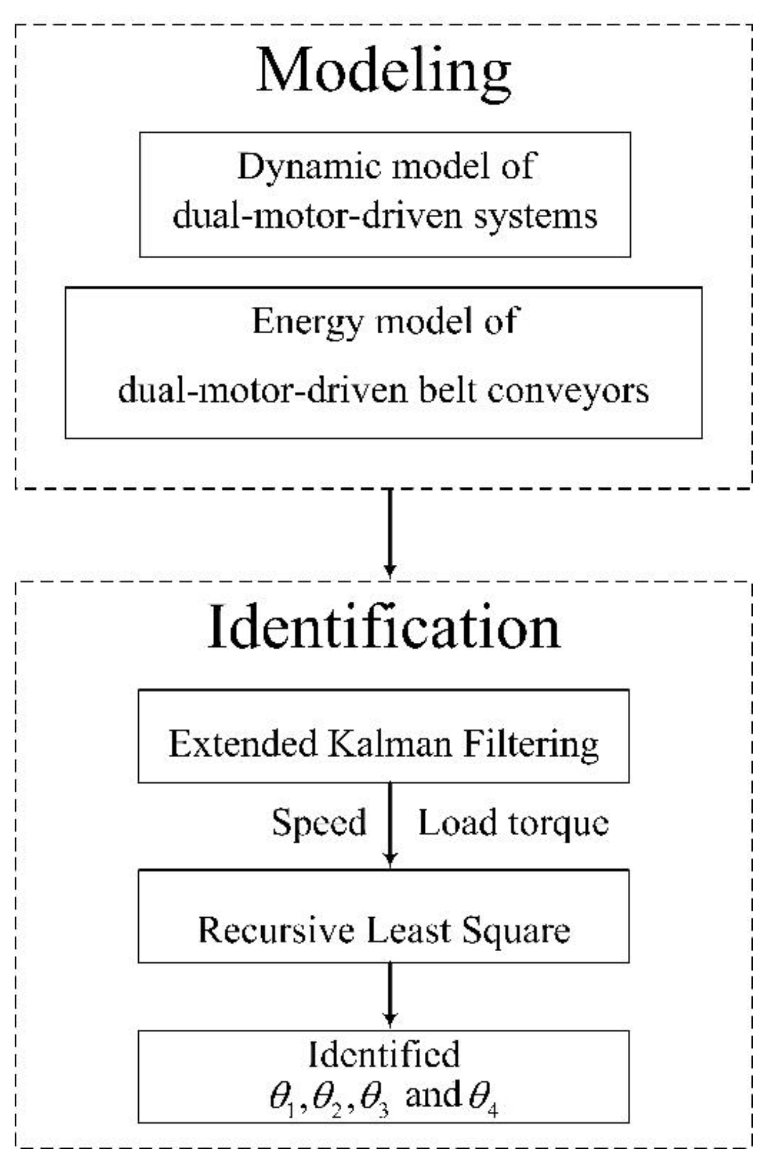
Figure 3.
Dual-motor-driven transmission system.
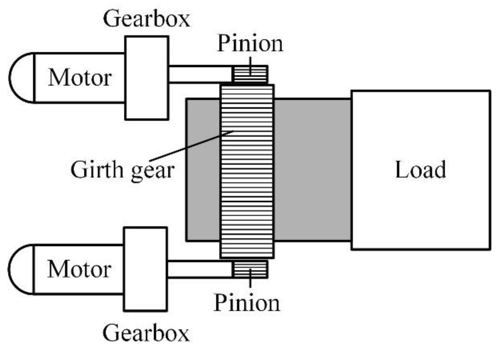
Figure 4.
Parameter identification scheme based on EKF and RLS.

Figure 5.
The scheme of EKF.

Figure 6.
The estimated value of motor speed.
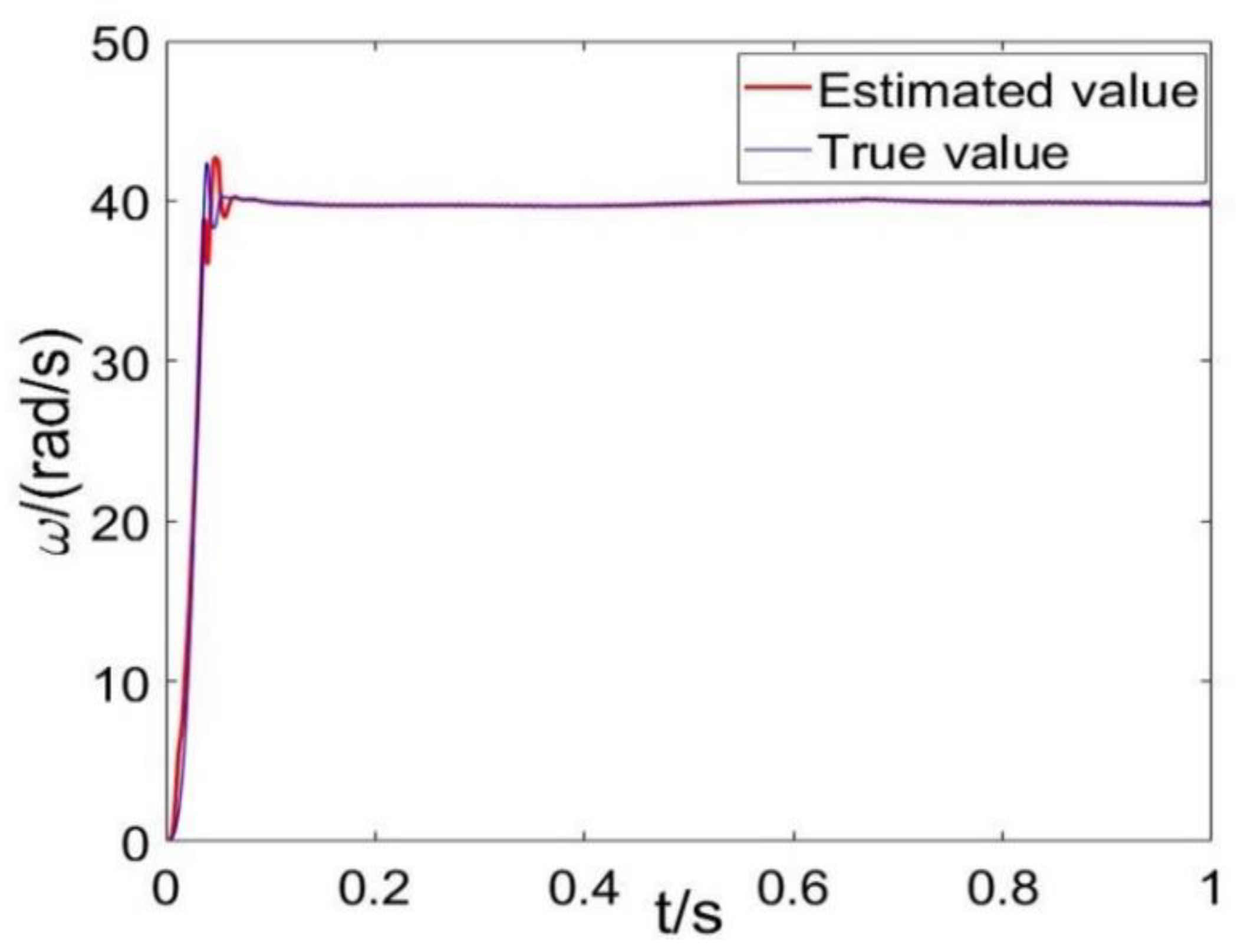
Figure 7.
The estimated value of load torque.
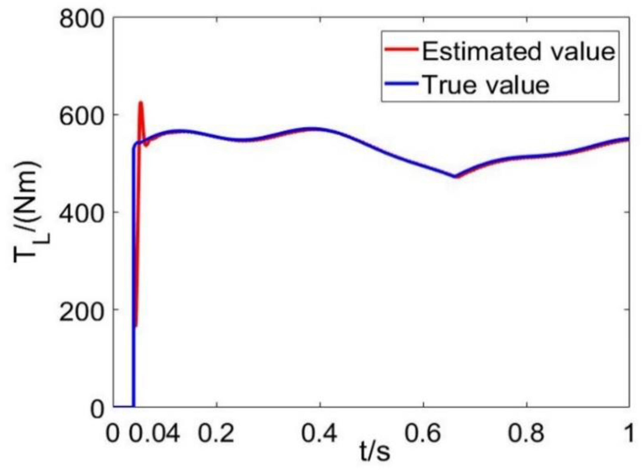
Figure 8.
The results of parameter identification.

Table 1.
Motors parameters list.
| Parameter | Value | Parameter | Value |
|---|---|---|---|
| 0.069 H | 0.070 H | ||
| 0.071 H | 0.073 H | ||
| 0.079 H | 0.080 H | ||
| 0.087 H/Ω | 0.088 H/Ω | ||
| 0.435 Ω | 0.437 Ω | ||
| 0.816 Ω | 0.815 Ω | ||
| 0.19 (N·m·s2) | 0.192 (N·m·s2) | ||
| 2 |
Table 2.
The results of parameter identification and true values.
| Parameters | ||||
|---|---|---|---|---|
| Identified value | 8566.3 | 0.0031 | 51.6804 | |
| True value | 8550.9 | 0.0032 | 51.2986 | |
| error | 3% | 0.18% | 3.23% | 0.74% |
© 2018 by the authors. Licensee MDPI, Basel, Switzerland. This article is an open access article distributed under the terms and conditions of the Creative Commons Attribution (CC BY) license (http://creativecommons.org/licenses/by/4.0/).
Share and Cite
MDPI and ACS Style
Yang, C.; Liu, J.; Li, H.; Zhou, L. Energy Modeling and Parameter Identification of Dual-Motor-Driven Belt Conveyors without Speed Sensors. Energies 2018, 11, 3313. https://doi.org/10.3390/en11123313
AMA Style
Yang C, Liu J, Li H, Zhou L. Energy Modeling and Parameter Identification of Dual-Motor-Driven Belt Conveyors without Speed Sensors. Energies. 2018; 11(12):3313. https://doi.org/10.3390/en11123313
Chicago/Turabian StyleYang, Chunyu, Jinhao Liu, Heng Li, and Linna Zhou. 2018. "Energy Modeling and Parameter Identification of Dual-Motor-Driven Belt Conveyors without Speed Sensors" Energies 11, no. 12: 3313. https://doi.org/10.3390/en11123313
Note that from the first issue of 2016, this journal uses article numbers instead of page numbers. See further details here.