Phase Balancing Home Energy Management System Using Model Predictive Control

Abstract

Most typical distribution networks are unbalanced due to unequal loading on each of the three phases and untransposed lines. In this paper, models and methods which can handle three-phase unbalanced scenarios are developed. The authors present a novel three-phase home energy management system to control both active and reactive power to provide per-phase optimization. Simplified single-phase algorithms are not sufficient to capture all the complexities a three-phase unbalance system poses. Distributed generators such as photo-voltaic systems, wind generators, and loads such as household electric and thermal demand connected to these networks directly depend on external factors such as weather, ambient temperature, and irradiation. They are also time dependent, containing daily, weekly, and seasonal cycles. Economic and phase-balanced operation of such generators and loads is very important to improve energy efficiency and maximize benefit while respecting consumer needs. Since homes and buildings are expected to consume a large share of electrical energy of a country, they are the ideal candidate to help solve these issues. The method developed will include typical distributed generation, loads, and various smart home models which were constructed using realistic models representing typical homes in Austria. A control scheme is provided which uses model predictive control with multi-objective mixed-integer quadratic programming to maximize self-consumption, user comfort and grid support.

1. Introduction

The Energy Efficiency Directive of the European Commission provides great emphasis on the need to empower and integrate customers by considering them as key entity towards sustainable and energy efficient future [1]. Evolving systems such as smart meters are on a road map towards increased market integration. With the help of such devices, ICT aspects such as data mining, management, processing, and commutation are gaining lots of traction in smart grid [2].

In recent days, with rigorous funding and investment in renewable energy, large number of distributed energy resources such as photo-voltaic systems, wind generators, and new loads such as electric mobility and storage systems are gaining importance. They pose lots of challenges to the network such as voltage violations and line loading. Most of the typical distribution networks are unbalanced due to unequal loading on each of the three phases and untransposed lines [3]. Additionally, unbalance is further increased with the high penetration of single-phase distributed generators. Three-phase unbalance imposes various degrees of stresses on different components in distribution network. Losses on the lines and distribution transformers increase considerably with the increase in phase unbalance [3]. Therefore, it is extremely important to consider three-phase models. They have strong dependencies on external factors such as weather, ambient temperature, and irradiation which follows daily, weekly, and seasonal cycles. Photo-voltaic systems inject large amounts of active power into the network, especially when the solar irradiation is high during midday. Voltage violations may occur due to partial stochastic power input. Therefore, it is important to include reactive power in models so that it can be used to performed voltage regulation.

Homes and buildings are projects to consume a large share of total energy production. Therefore, it makes sense to produce strategies to use them to help mitigate the issues discussed above. Most of the homes today are not capable of providing any kind of support to the grid. Certain upgrades need to be made so that they can perform demand response. Loads which can be controlled directly or indirectly to provide demand response is referred to as demand side management (DSM). DSM is also referred to as flexibility. DSM can be used to provide number of grid support functionalities such as shifting the peak load to off-peak hours or curtailing the load to reduce the peak demand [4]. Smart building customers are given the opportunity to schedule the devices on their own to maximize comfort level and based on this initial schedule, the optimizer maximizes economic return which will result in demand which is more leveled over time [5]. Additionally, the optimizer will either minimize payment or maximize comfort based on the consumer needs in which, the user comfort is represented as a group of linear constraints [6].

2. Related Work

To control various devices in smart homes and all the issues associated with it, the authors in paper have presented a control scheme using Model predictive control, which is an ideal candidate to handle dynamic systems with evolving disturbances described in the previous section.

Various implementations of model predictive controller (MPC) in buildings are available in the literature. The core principle or issue being addressed by bodies of research mentioned below is dynamic scheduling of various flexibilities in building. Most of the authors below have addressed this issue using various MPC algorithms, problem formulations and objectives.

After analyzing the large body of work in MPC for buildings, three major categories can be defined. MPC in buildings is mainly used for demand side and flexibility management, building temperature control and optimal usage of energy.

2.1. Demand Side and Flexibility Management

A multi-scale stochastic MPC is implemented to schedule heating, ventilation, air conditioning which is referred to as HVAC systems and controllable loads such as electric vehicles and washer/dryers is implemented in [7]. In [8], the authors have presented an MPC approach to tackle the load shifting problem in households equipped with controllable appliances and electric storage units. This approach used time of day tariff to minimize energy consumption. A decision-making framework for real time control of load serving entity of flexibilities used to provide ancillary services to the market is presented in [9]. This paper provides a generalized framework which includes wide array of flexibilities. An example with electric vehicle charging is provided in detail.

The authors in [10] have proposed a scheme which uses time varying real time pricing to schedule appliances in buildings in smart grid context. Thermal mass of the building is considered with a comfort indicator and a model associated with it is presented. Thermal mass storage is used to hedge against varying prices with a goal to minimize energy costs. Control approach for home energy management system (HEMS) under forecast uncertainty is presented in [11]. The smart home is controlled as a grid connected micro-grid with PV generation, battery systems, critical and controllable loads. Objective of MPC is to maximize the use of renewable energy generation and to minimize operation costs. It includes predictions of PV, load, and market prices. Various scenarios are considered with different forecasting accuracies.

The authors in [12] presented an MPC model for HVAC system in medium sized building with receding horizon control. It is used to provide demand side flexibilities. Objective is to operate the building economically while respecting the comfort of dwellers. MPC scheme provided is a robust one to participate in both reserve and spot markets. Sensitivity of the controller towards economic and technical constraints are evaluated. The National Electricity Market of Singapore (NEMS) is used as a study case for grid building integration studies.

In [13], a non-intrusive identification of components in smart home is provided with a sampling frequency of one hertz. These identified models are used to predict flexibilities. These flexibilities are shifted in time to minimize energy costs. An MPC technique for energy optimization in residential appliance is proposed in [14]. Home cooling and heating system control is proposed to analyze the effect of conventional thermostats. In [15], an MPC EMS system for residential micro grids is furnished. EMS optimally schedules smart appliances, heating systems, PV generators based on consumer preferences. Weather and demand forecasts are integrated in it. Mixed-integer linear programming (MILP) is the core of MPC which minimizes the system costs of this residential micro-grid. At each sample time, the optimization algorithm adjusts itself to account for updated weather dependent PV systems and heating units in a receding fashion. This method is coupled with accurate simulation of micro-grid including energy storage and flexible loads. Emulation of real-world grid conditions on standard network interface is presented. The authors in [16] have provided a method to maximize the use of renewable energy resources in islanded grids. PV systems are used to provide energy to home loads and pico hydro power plant. MPC is used to control the flow valve of hydro plant and to modulate the energy supply to fulfill the deficit during islanded conditions.

An economic MPC is illustrated in [17]. It includes PV combined heat and electrical storage system. Uncertainties from thermal behaviors of the building are quantified, formulated and MPC’s capability to handle it is presented in this research work. An MPC scheme to control loads in residential buildings are presented in [18]. It also presents a novel load aggregation method using MPC for distribution networks. This method is tested with 342 bus network with 15,000 buildings. In [19], an MPC controller to perform demand side management is presented. It uses an ON/OFF PID controller and MPC to control air conditioning in rooms in houses. It also includes PV systems. Weekly expenses are calculated for each tariff is compared with control methods.

2.2. Temperature Control

The authors in [20], have presented a method to control temperature in building in a cost-effective manner. It uses linear programming heuristic to minimize the objective function of electricity cost to run air conditioning system. In [21], authors have presented models for Heat Recovery Ventilators connected to single zone building, its potential and nonlinear MPC is implemented to optimize energy consumption. Three distinct time zones are used namely, slow timescale for temperature of structural elements, fast timescale for air temperature and intermediate dynamics for recovery systems. A stochastic optimization technique is provided in [22]. This paper introduces several load classes such as heating, ventilation, air conditioning which is commonly referred to as HVAC systems. A first order thermal dynamic model is used with a mixed-integer MPC to generate load schedules. Real data is coupled with numerical solutions. The authors in [23] have proposed an MPC algorithm to control temperature in single zone building coupled with renewable energy generators such as solar and wind. MPC objective is to control temperature within certain permissible limits and optimal amount of power consumption.

In [24], a temperature control scheme with the consideration of occupants with three comfort indicators namely, strict, mild, loose levels are provided. It also includes window blind position control, illumination, and ambient temperature. Weather data such as solar irradiation, illumination, and ambient temperature is forecasted and used in MPC algorithm. Goal of MPC is to minimize energy consumption and maintain the desired level of comfort for occupants. Paper [25] focuses on analysis of MPC application to domestic appliances to optimize them. Relationship between MPC weight adjustment and minimization of energy consumption is evaluated. In this context, water heater, room temperature control by air conditioning system and refrigerators are explored.

In [26], a centralized direct control of on/off thermostats is furnished. Device operation temperature, on/off status, more importantly, temperature ramps are calculated and communicated to the central controller. It is observed that, same or better performance can be achieved by communication of temperature ramps which are essential data points. It also reduces the communication needs significantly. Right information exchange is essential for better performance and data flow reduction is the concluding argument of this paper.

An MPC control scheme to provide the best tradeoff between temperature control and energy cost is described in [27]. It also provides a comparison between PID controller and MPC. The weights are modified to obtain the best solution to increase quality of various electrical and thermal models. The authors in [28], have presented an MPC for entire building with a comfort metric to ensure high priority to user comfort for each of the various zones in the building. Simulation results are provided for four months showing large percentage of reduction in electrical and thermal energy consumption.

2.3. Optimal Energy Usage

Paper [29] proposes an MPC control strategy in HEMS to optimize energy usage and optimal operational schedules for input variables. It also provides results which demonstrated revenue from selling power to the utility. In [30], authors have furnished an MPC approach to obtain savings in residential households. Impact of local power generation such as roof top PV systems is determined for off-peak, mid-peak and on-peak periods. Hybrid MPC formulation for buildings is provided in [31]. It describes the interactions between continuous and discrete systems. It involves a two-level computation structure. Individual systems are controlled with upper level discrete commands.

In [32], an approach to minimize energy in home and office building is presented with renewable energy resources such as PV systems. This is done using an MPC technique with mixed-integer programming to handle switching constraints. This method allows for sufficient performance with respect to energy regulation and efficiency. It is shown that with various seasons, an annual savings of about 1.72% can be achieved with this approach. An MPC approach is introduced in [33] which exploits its capacity to reduce energy consumption and improve efficiency to reduce energy bills. MPC was trained for two different weight sets which is compared to thermostat control with three typical household loads.

It is shown that it is necessary to augment control weights to maximize energy cost minimization potential. In [34], an energy scheduling approach for smart home appliances using stochastic MPC is presented. It comprises a combination of genetic algorithm and linear programming. It analyzes the competence of the algorithm proposed with the objective of energy reduction.

An MPC scheme with a sample time of one hour is presented in [35]. It includes hot water usage, electric vehicle, domestic heating and with an actuator with water tank to use it as heat storage. Total power and energy cost is minimized. MPC robustness is evaluated using forecasted load profiles of the household. It is shown that using energy storage, the overall energy consumption of the household can be minimized.

A comprehensive cost optimal design is presented for a building HVAC system which includes MPC to generate cost optimal solution is presented in [36] The controller provides an optimal hourly set point for cooling and heating devices. This method is applied to multi-zone building in Italy. In [37], a study to minimize the cost of electricity for coordinating houses connected a micro-grid. It uses multi-objective optimization for micro-grid control which includes a house and an independent local plant. The control algorithm minimizes losses by power exchanges between the plant and the house.

It can be clearly seen that, three-phase implementation of HEMS is lacking. The papers mentioned above only use simple single-phase flexibility models and appliances are single phased. Additionally, reactive power control is not addressed by any of the research work mentioned above. Since three-phase models are not used, phase unbalance minimization cannot be performed. In this paper, the authors present a three-phase unbalanced HEMS in which, three objective functions, maximize user comfort, self-consumption and grid support is implemented. It also includes control scheme to manage both active and reactive powers and can handle number of electrical appliances with various configurations.

The contributions in this paper are enlisted below,

• Various three-phase linear flexibility models are presented in Section 3.
• Flexibilities are modeled in both active and reactive power.
• Three objective functions are provided in Section 5 along with three objective weights which are user defined.
• Control scheme is described in Section 6 for three-phase HEMS with various chronological events.
• Simulation results for three-phase unbalanced HEMS with active and reactive power control is provided in Section 7.

3. System Models

HEMS is a platform which enables monitoring and control of various energy appliances in the household. It allows the deployment of various control strategies to achieve an objective. Smart home in this paper refers to a home which is fitted with a HEMS. Using this system, various objectives can be achieved. For example, keeping the room temperature within certain comfortable limits.

3.1. Overview

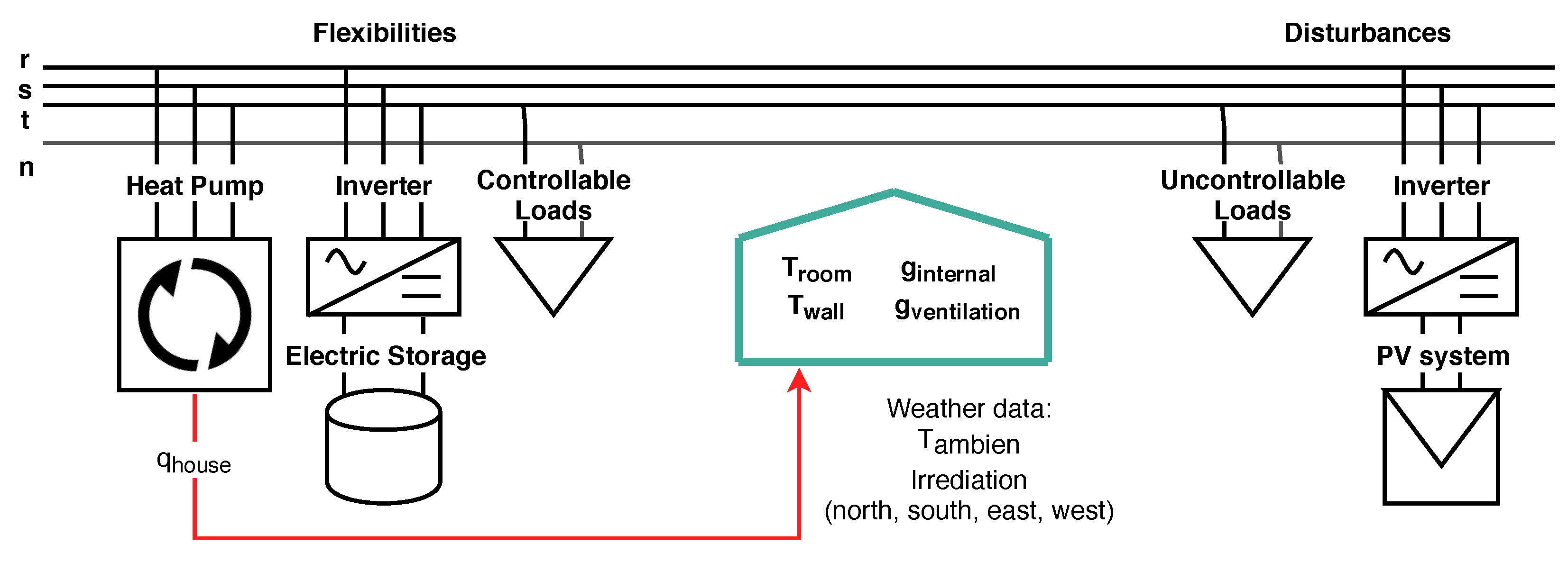
Smart home models can be segregated into two categories. Namely, thermal and electrical models coupled by a heat pump. The main reason to use a thermal model is to characterize indoor temperature due to the thermal inertia of the house, since consumer comfort is paramount. The controller is formulated to give complete control to the user, a user-centric approach. The models are linear in nature so that, simple control strategies can be produced. Figure 1 represents a three-phase HEMS. It contains both single and three-phase components and therefore, it is unbalanced. In this scenario, the heat pump is three phased, inverters for battery and PV are three phased, controllable, and uncontrollable loads are single phased. The control scheme provided in this paper can include variety of configurations such as single-phase—neutral, phase—phase, three-phase star configuration, three-phase star configuration with neutral, and three-phase delta configuration. This can be done using the constraint imposed on the grid connection point described in Section 4.4.

3.2. Smart Home Thermal Model

Various linear single zone models representing single family homes with heat pumps and thermal parameters of the building are considered. They are based on nonlinear models which were constructed using data, representing physical behavior of real buildings in Vienna and Salzburg regions in Austria. Due to consumer privacy, more details about these homes cannot be provided. By generalizing these models, four study cases are derived, and their essential distinguishing features are shown in

Table 1. Building study cases which represent typical households in Austria. During the modeling stage of these houses, they only contained single-phase loads. To perform effective demand response, they had to be upgraded to include various other flexibilities such as single/three-phase heat pumps, controllable loads, electric storage, and PV system with three-phase inverters. Some of the important specifications such as heat demand, control method, and rated capacities which influences the control scheme are provided in this table.

House Hype	Passive House	Low-Energy House	Existing House	Renovated House
Heating demand	15 kWh/(m2a)	45 kWh/(m2a)	100 kWh/(m2a)	75 kWh/(m2a)
Heater	Under floor	Under floor	Radiator	Radiator
Heat exchange medium	Air-water	brine-water	brine-water	air-water
Power control	Variable	On/off	On/off	Variable
Rated capacity	1 kW/ 3 kW	1.2 kW/5 kW	4 kW/12kW	2.7 kW/7 kW
(Electrical/thermal)

. Nonlinear models were created in Dymola [38], which is a modeling and simulation tool, as part of the project iWPP-Flex [39]. They were linearized using the functions within Dymola and were mathematically verified.

In the context of smart HEMS, the models of smart homes are recommended to be kept sufficiently simple to maintain generality, so that many building types can be accommodated. Therefore, first order models are implemented. Additionally, the focus of this work is not to use realistic building models but rather the control strategy and to minimize the objective function.

As a result, continuous state space models were generated and are assumed to be ordinary discrete linear time-invariant and is then discretized with a sampling time step of 15 min which can be observed in Equation (1).

$$x_{room}(t+1)=A_{room}{x}_{room}(t)+B_{room}{u}_{room}(t)$$

(1)

The state variables $x_{room}$ of the building model are the room and wall temperature. The later represents the temperature of wall, floor, and ceiling of the house. $A_{room}$ and $B_{room}$ are the system matrices.

$$x_{room}=\left[\begin{array}{c}{T}_{wall}\\ T_{room}\end{array}\right]$$

(2)

Limits on room and wall temperatures are given in Equations (3) and (4)

$$T_{wall}^{min}\le T_{wall}(t)\le T_{wall}^{max}$$

(3)

$$T_{room}^{min}\le T_{room}(t)\le T_{room}^{max}$$

(4)

The input quantities for the building are heat flow supplied by the heat pump, ambient temperature, solar irradiation from all directions, internal gains, and ventilation.

$$u_{room}=\left[\begin{array}{c}{q}_{room}\\ T_{ambienttemperature}\\ i_{north}\\ i_{east}\\ i_{south}\\ i_{west}\\ g_{internalgain}\\ g_{ventilation}\end{array}\right]$$

(5)

Limits on heat flows into the building are provided in Equation (6)

$$0\le q_{room}(t)\le q_{room}^{max}$$

(6)

3.3. Heat Pump in Residential Building

Heat pump is used to provide the heat flow into the home which is the only controllable variable in the home model described in Section 3.2. Heat pump is the only coupling element between electrical and thermal systems as mentioned above.

Equation (7) describes the relationship between heat pump power and heat flows. The model represented below is that of a single-phase heat pump since it is in a modest home. This can be easily extended to three-phase by dividing the right-hand side of Equation (7) by 3 for per-phase balanced active power. Coefficient of performance ($cop$) is assumed to be constant with respect to time.

$$P_{heatpump}(t)=\frac{q_{room}(t)}{co{p}_{heatpump}}$$

(7)

Where, $P_{heatpump}$ is the active power and $co{p}_{heatpump}$ is the coefficient of performance. Low-energy and existing house contains on-off heat pump. To model this, a binary variable $B_{heatpump}$ with 0 for off and 1 for on is used.

$$P_{heatpump}(t)=B_{heatpump}{P}_{heatpump}^{rated}$$

(8)

The pump in heat pump consists of an induction motor. This motor is assumed to be lossless and with constant power factor ($p{f}_{heatpump}$) as described in Equation (9), using which reactive power ($Q_{heatpump}$) is calculated.

$$Q_{heatpump}(t)=tan(co{s}^{-1}(p{f}_{heatpump}))P_{heatpump}(t)$$

(9)

Since only heating period is considered, $P_{heatpump}$ and $Q_{heatpump}$ ≥ 0. Constraints on heat pump active power limits.

$$0\le P_{heatpump}(t)\le P_{heatpump}^{max}$$

(10)

Constraints on heat pump reactive power limits,

$$0\le Q_{heatpump}(t)\le Q_{heatpump}^{max}$$

(11)

where, $P_{heatpump}^{max}$ and $Q_{heatpump}^{max}$ are the maximum rated power active and reactive powers of head pump, respectively.

4. Electrical System Constraints

In recent years, lots of smart electrical appliances are becoming popular. It is possible to control the behavior of these appliances. In this paper, the authors have decided to use the following electrical appliances.

4.1. Electric Storage Constraints

For the maximal use of intermittent renewable energy generators and self-consumption, electric batteries are becoming very important in the recent days. Therefore, it is necessary to model and include them in the HEMS systems. In this paper, only linear battery models are used. Equation (12) represents the energy balance of electric storage system, a battery.

$$soc(t+1)C_{battery}=soc(t)C_{battery}+\Delta t{\eta }_{battery}{P}_{battery}(t)$$

(12)

It can be seen in Equation (12) that, $P_{battery}$ takes values both positive and negative. This is a form of linearization because, the battery charging and discharging efficiencies are different and therefore, nonlinear. This nonlinearity can be tackled by solving it as is, using a nonlinear solver or by splitting the $P_{battery}$ into $P_{charging}$ and $P_{discharge}$. The latter is coupled with a binary variable to make it either charge or discharge, leading to MILP. The authors have chosen to use the linear form and the reasons for it are provided in Section 4.2.

Constraints on soc limits are given below,

$$so{c}^{min}\le soc(t)\le so{c}^{max}$$

(13)

Constraints on battery charging and discharging power limits are as follows.

$$P_{battery}^{min}\le P_{battery}(t)\le P_{battery}^{max}$$

(14)

4.2. Three-Phase Inverter Constraints

The battery described in the previous section is connected to a three-phase inverter. The inverter can control active and reactive power flows on each of the phases. The relationship between battery and inverter is described using simple power balance Equation (15).

$${(P_{battery}(t))}^2={(P_{inverter}(t))}^2+{(Q_{inverter}(t))}^2$$

(15)

Equation (15) is nonlinear. If on the precious section, a binary variable is defined and $P_{battery}$ is split into $P_{charging}$ and $P_{discharge}$, Equation (15) becomes nonlinear and non-convex. One way to deal with the nonconvexity is to limit the $Q_{inverter}$ with a constant power factor as shown in Equation (16). However, this is still nonlinear.

$$Q_{inverter}^{\rho }(t)=tan(co{s}^{-1}(p{f}_{inverter}))P_{inverter}^{\rho }(t)$$

(16)

where, $\rho$ is the phase and $\rho \in phases(r,s,t)$. To remedy the nonlinearity, the inverter is only controlled at unity power factor. In other words, the reactive power is zero. This is represented in Equation (17)

$${(P_{battery}(t))}^2={(P_{inverter}(t))}^2$$

(17)

Individual phase powers are represented as follows,

$$P_{inverter}(t)=\sum _{\rho }{P}_{inverter}^{\rho }(t)$$

(18)

4.3. Constraints on Controllable Loads

Simple controllable loads are used with constant power factor operation as described in Equation (21). Controllable loads have the following constraints. Equations (19) and (20) are the active and reactive power constraints and Equation (21) is the relationship between them.

$$0\le P_{controllableload}^{\rho }(t)\le P_{controllableload}^{max}$$

(19)

$$0\le Q_{controllableload}^{\rho }(t)\le Q_{controllableload}^{max}$$

(20)

It is assumed that the power factor is constant with time. Typical power factor for household loads is between 0.90 to 0.95.

$$Q_{controllableload}^{\rho }(t)=tan(co{s}^{-1}(p{f}_{controllableload}))P_{controllableload}^{\rho }(t)$$

(21)

4.4. Constraints on Grid Connection Point

The grid connection point (point of common coupling) is where the smart home is connected to the grid. When excess power is fed into the grid, it is referred to as infeed and when power is drawn, it is referred to as consumption. Since $P_{grid}$ takes both positive and negative values due to battery linearization, both infeed and consumption is represented by $P_{grid}$. It also represents the energy balance of all the electrical components in the smart home.

Equations (22) and (23) are constraints on limits of active and reactive power at the grid connection point.

$$P_{grid}^{\rho }(t)=P_{inverter}^{\rho }(t)+P_{heatpump}^{\rho }(t)+P_{controllableload}^{\rho }(t)+P_{uncontrollableload}^{\rho }$$

(22)

$$Q_{grid}^{\rho }(t)=Q_{heatpump}^{\rho }(t)+Q_{controllableload}^{\rho }(t)+Q_{uncontrollableload}^{\rho }$$

(23)

4.5. Various Disturbances Applied to HEMS

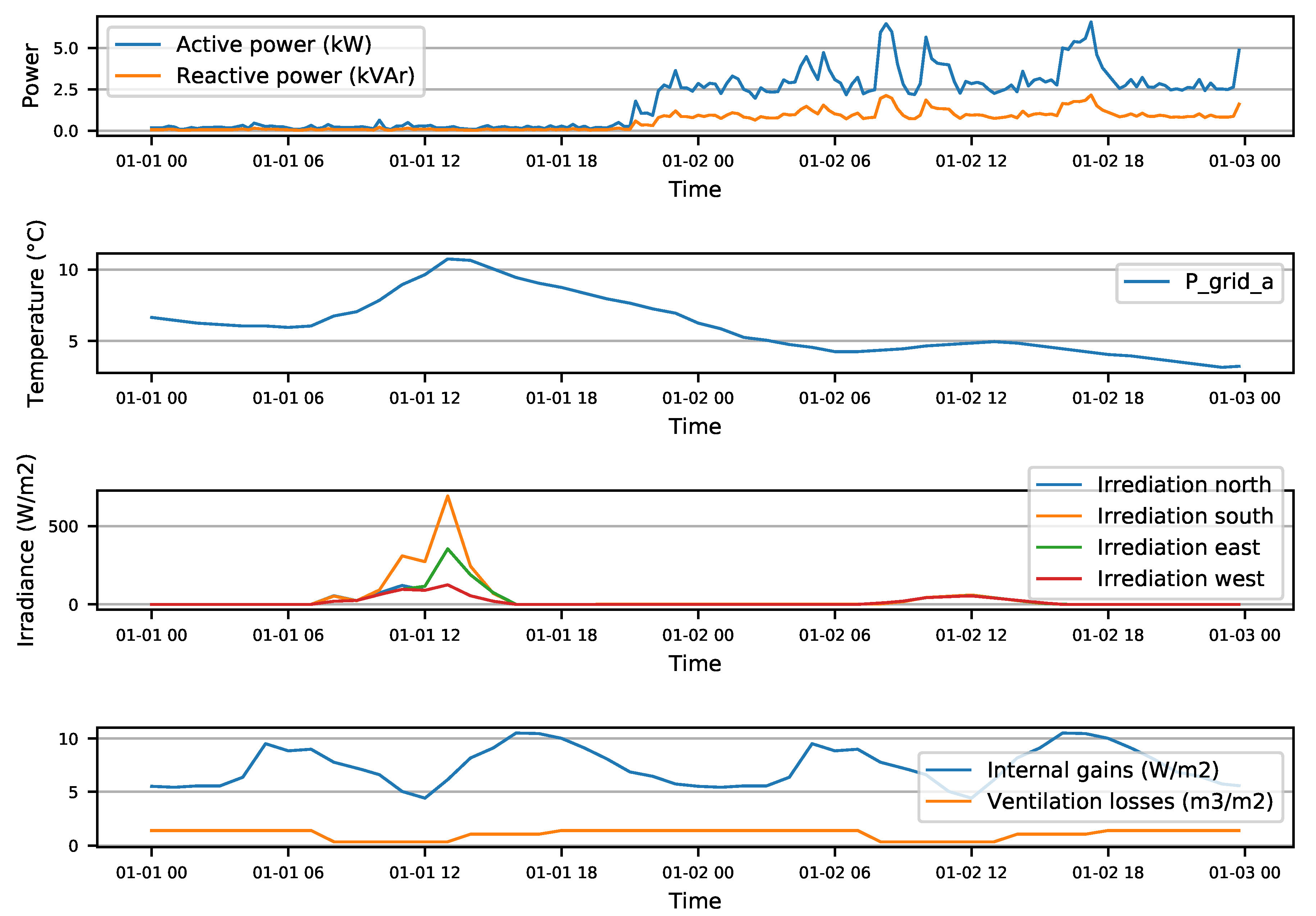
Various electrical and thermal disturbances are applied to HEMS during simulation which can be seen in Figure 2.

Disturbances are forecasted using a convolutional neural network which is not described in this paper. Uncontrollable loads data is from a smart meter from a real household in Austria. Various thermal disturbances such as ambient temperature and irradiation data is sourced from weather stations in Austria, ventilation, and internal gains from the project iWPP-Flex.

5. Objective Functions

In this paper, three different objectives are considered. These are explained in detail below.

5.1. Improve Self-Consumption

In many countries, with higher share of renewables, it is more economical to self-consume and therefore, the following objective function in Equation (24) is minimized. Since electricity tariffs only depend on active power, reactive power is excluded from the objective.

$$J_{selfconsumption}=\sum _t\sum _p{(P_{grid}^{\rho }(t))}^2$$

(24)

On the other hand, in Austria, it is more economical to feed as mush power into the grid as possible since power sale tariff is higher than consumption tariffs. It can be done easily by maximizing equation. It is customary to involve a variable price signal along with $P_{grid}$ which is the electricity tariff provided by the energy retailer. However, this is neglected for the sake of clarity.

5.2. Improve User Comfort

Since user comfort is paramount, this objective is introduced. It minimizes the difference between a reference temperature and actual room temperature in smart home. The limits of these temperature are defined by the user.

$$J_{usercomfort}=\sum _t{(T_{room}^{reference}(t)-T_{room}(t))}^2$$

(25)

5.3. Improve Grid Support

As mentioned in Section 1, smart homes can provide support to the grid by optimally controlling its renewable generation and consumption. Therefore, objective in Equation (26) is provided. It minimizes the difference between reference and actual active, reactive powers at grid connection point. This reference is generated from a large grid level optimal power flow controller based on a grid level objective function.

$$\begin{array}{cc}\hfill J_{gridsupport}=\sum _t\sum _p& {(P_{gridreference}^{\rho }(t)-P_{grid}^{\rho }(t))}^2+{(Q_{gridreference}^{\rho }(t)-Q_{grid}^{\rho }(t))}^2\hfill \end{array}$$

(26)

This paper does not include details or methods to generate this reference profile and instead uses it as is. If the smart home can follow this reference profile, grid level optimization is achieved. The objective on the grid can be loss minimization, line loading minimization, operational efficiency, unit dispatch and so on. In this paper, the reference profiles where generated with an objective to minimize the three-phase unbalance on the grid level. For this to work, multiple buildings connected at various locations in the network must follow its own reference profile provided by the grid controller, simultaneously.

5.4. Complete Objective Function

Complete objective function is provided in Equation (27). Weights $\mathcal{S}$, $\mathcal{U}$ and $\mathcal{G}$ are introduced with self-consumption, user comfort and grid support, respectively. By varying these weights, more importance can be given to the objectives.

$$minimizeJ=\mathcal{S}{J}_{selfconsumption}+\mathcal{U}{J}_{usercomfort}+\mathcal{G}{J}_{gridsupport}$$

(27)

These weights can be varied on-line and the controller updates it in the next simulation step. There are the most prominent parameters which the user can determine and can have significant influence over the controller and ultimately the optimum. Controllable variables are $P_{battery}$, $P_{heatpump}$ and $P_{controllableload}$.

6. Control Scheme

Due to the high intermittency of renewable energy generators, loading in households along with dependencies on external factors such as weather and solar irradiation, it is extremely important to choose a controller which makes effective use of available predictions.

Therefore, the authors have chosen to use MPC. MPC control used is receding horizon control. Figure 3 describes an MPC and data exchange between various devices in smart home. MPC is responsible to generate optimal set-points to minimize the objective function.

MPC control scheme is illustrated in Figure 4. It describes various functions which need to be executed within a sample duration.

The chronological control functions and events described in Figure 4 are described in detail below.

• At time t, measure thermal disturbances such as irradiation, ambient temperature, ventilation losses and internal gains. Additionally, smart meters measures uncontrollable load and photo-voltaic generation.
• These sensor data points are acquired by the data acquisition system and sensor database is updated. Figure 5 illustrates the sensor data acquisition system using in this work.
• Disturbances are forecasted for a given prediction horizon using an appropriate forecasting algorithm. In this paper, using convolutional neural networks.
• Active and reactive power optimal set-points are received from the grid level controller.
• Internal temperature reference signals are received.
• User defined objective weights are received.
• Objective functions are set up using Equations (24)–(27).
• Constraints from Equations (1)–(23) are setup.
• Optimal set-points are generated.
• The process is repeated for next sample period, $(t+1)$.

The optimization problem is solved by a suitable quadratic programming for passive, renovated house and mixed-integer quadratic programming for low-energy and existing houses as discussed in Section 3.3.

7. Simulation Results

In this section, simulation setup and results are provided. As mentioned earlier, the objective weights, $\mathcal{S}$, $\mathcal{U}$ and $\mathcal{G}$ are defined by the user, it is difficult to analyze the controller performance due to large number of combinations of these three variables.

To overcome this, only extreme cases of these weights are considered. This can be observed in Figure 6. The method of choosing weights in such fashion was inspired from [40] in which, mixed-integer quadratic programming is introduced with multi-objective optimization. The simulation is performed for the duration of 48 hours with prediction and control horizon of 24 hours.

Simulation parameters are provided in

Table 2. Simulation parameters.

Variable	Value
Simulation parameters
prediction horizon	24 h
control horizon	24 h
simulation duration	48 h
Building model
$T_{wall}^{min}$	10 C
$T_{wall}^{max}$	40 C
$T_{room}^{min}$	18 C
$T_{room}^{max}$	25 C
$T_{initial}$	18 C
$T_{room}^{reference}$	20 C
Controllable load model
$P_{controllableload}^{max}$	2 kW
$p{f}_{controllableload}$	0.95
Electric Storage model
$so{c}^{min}$	0.3
$so{c}^{max}$	0.9
$C_{battery}$	20 kWh
${\eta }_{battery}$	0.95
$P_{battery}^{min}$	–10 kW
$P_{battery}^{max}$	10 kW
Heat pump model
$cop$	3
$p{f}_{heatpump}$	0.90
Passive house: $P_{heatpump}^{max}$	1 kW
Low-energy house: $P_{heatpump}^{max}$	1.2 kW
Existing house: $P_{heatpump}^{max}$	4 kW
Renovated house: $P_{heatpump}^{max}$	2.7 kW

.

7.1. Analysis of Results

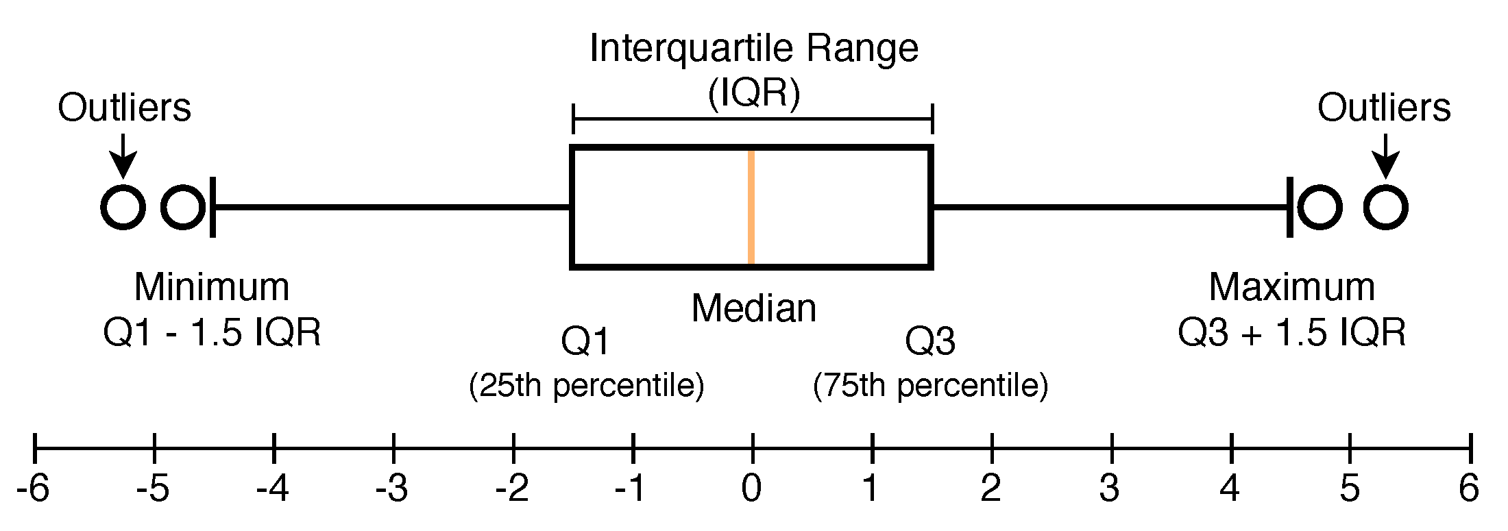
Due to the large number of combinations of objective weights and controllable variables, results are analyzed based on the three objective functions. Four scenarios of objective weights are chosen for analysis. ($\mathcal{S}$, $\mathcal{U}$, $\mathcal{G})=$$(0,0,1)$, $(0,1,0)$, $(1,0,0)$ and $(1,1,1)$. Additionally, to represent powers, only phase r is used. The results are plotted using boxplots. More information about it can be seen in Figure 7.

7.1.1. Improve Self-Consumption

Figure 8 describes the results for the objective function to minimize self-consumption (see, Equation (24)). It illustrates $P_{grid}$ for various home types and for given simulation horizon. It can be observed that for objective weights ($\mathcal{S}$, $\mathcal{U}$, $\mathcal{G})=(1,0,0)$, the controller is trying to get $P_{grid}$ close to zero which can be perceived from the medians which are at zero for all the house types. Same can be observed with objective weights ($\mathcal{S}$, $\mathcal{U}$, $\mathcal{G})=(1,1,1)$. Since all three weights are equal, the results are not as effective as the one from before and $\mathcal{S}$ is not dominating other weights.

7.1.2. Improve User Comfort

Objective terms $abs(T_{room}^{reference}-T_{room})$ is illustrated in Figure 9. Since the objective weight $\mathcal{U}$ is predominant, ($\mathcal{S}$, $\mathcal{U}$, $\mathcal{G})=(0,1,0)$, the absolute difference between $T_{room}^{reference}$ and $T_{room}$ is the least. It can be observed that the temperature median is very close to zero. From this, it can be inferred that the objective function to improve user comfort is maximized. However, since the building models are first order, the controller is quiet easily able to achieve similar results with ($\mathcal{S}$, $\mathcal{U}$, $\mathcal{G})=(1,1,1)$.

7.1.3. Improve Grid Support

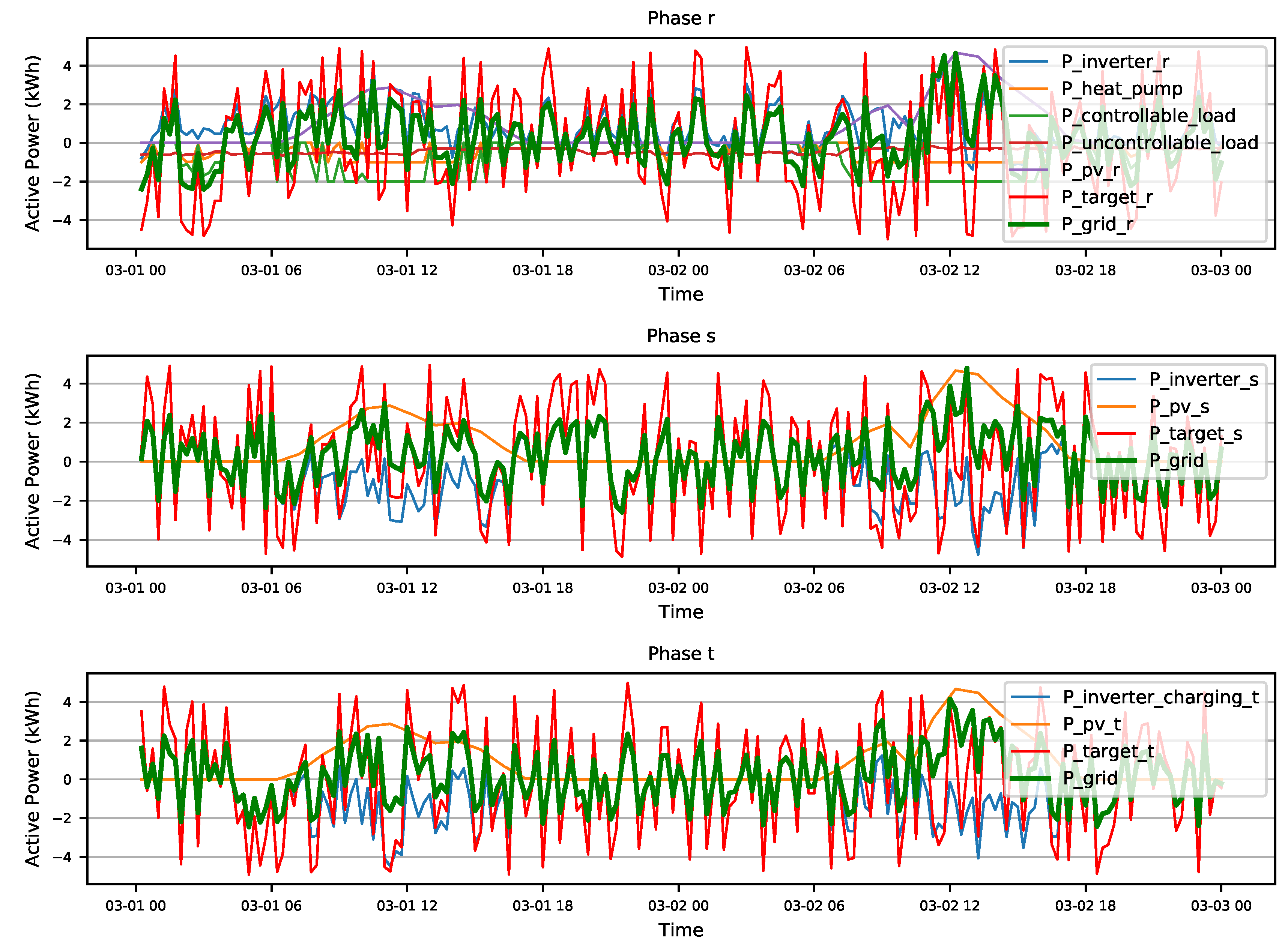
Figure 10 illustrates $abs(P_{gridreference}(t)-P_{grid})$. With the predominant weight in ($\mathcal{S}$, $\mathcal{U}$, $\mathcal{G})=(0,0,1)$ is $\mathcal{G}$. Therefore, similar to previous objectives, it can be observed that the controller is able to minimize the absolute difference between the target profile and the profile at the grid connection point. This is also illustrated in Figure 11 and Figure 12 where, both active and reactive power profiles are presented for phase r.

Figure 11 and Figure 12 describes all the parameters for passive house with objective weight scenario ($\mathcal{S}$, $\mathcal{U}$, $\mathcal{G})=(0,0,1)$ for both active and reactive power. In Figure 11, since the objective weight scenario is to minimize $abs(P_{gridreference}(t)-P_{grid})+abs(Q_{gridreference}(t)-Q_{grid})$, it can be observed that the $P_{grid}$ is trying to closely follow the $P_{gridreference}$.

It is evident from Equation (23) that, there are no direct reactive power controllable variables for all the phases. This makes it difficult for the controller to actively tract $Q_{gridreference}$ which can be observed in Figure 12. In phase r, due to the existing single-phase appliances, better reactive control tracking is possible unlike phase s and t.

8. Conclusions and Outlook

In this paper, a novel three-phase balancing HEMS was presented along with control strategies for both active and reactive power. Four linear building models representing typical households in Austria were described. Various linear three-phase flexibility models were presented in detail. Three unique conflicting objective functions with three weights which are user defined is described. Model predictive control scheme was applied to this smart home for various extreme objective weight scenarios. Active and reactive power set-points were generated for all electrical controllable variables. Due to the vast number of combinations of objective weights, four extreme cases were chosen for analysis, ($\mathcal{S}$, $\mathcal{U}$, $\mathcal{G})=$$(0,0,1)$, $(0,1,0)$, $(1,0,0)$ and $(1,1,1)$. Analysis was done based on three objective functions. It was shown that the results reflect the chosen objective weights for each of the three objective functions. In Figure 11 and Figure 12, grid support maximization objective was illustrated for objective weights ($\mathcal{S}$, $\mathcal{U}$, $\mathcal{G})=$$(0,0,1)$. In these figures, it was shown that $P_{grid}$ and $Q_{grid}$ are indeed able to track their reference profiles and implications being, the objectives on the grid level controller (three-phase unbalance minimization) are being met, leading to a grid level optimization.

The models presented in the paper were linear and first order in nature. In reality it makes sense to use higher order nonlinear models to closely match the real behavior of the smart home. Therefore, the model needs to be extended to nonlinear ones. Even though the scheme includes reactive power, it is not given high importance in this paper to keep it linear. Due to high share of renewable generators, it is interesting to be able to control reactive power in this context. The inverter connected to the battery in this paper only works at unity power factor. However, by including reactive power control, better reactive power tracking can be performed. Additionally, with the power balance equation at the inverter is non-convex in nature. Therefore, the MPC needs to be extended to be able to solve such problems using a non-convex solver.

References

- General, D. Energy Efficiency Directive. Available online: https://ec.europa.eu/energy/en/studies (accessed on 20 August 2018).
- Barbato, A.; Capone, A.; Barbato, A.; Capone, A. Optimization Models and Methods for Demand-Side Management of Residential Users: A Survey. Energies 2014, 7, 5787–5824. [Google Scholar] [CrossRef] [Green Version]
- Sun, Y.; Li, P.; Li, S.; Zhang, L.; Sun, Y.; Li, P.; Li, S.; Zhang, L. Contribution Determination for Multiple Unbalanced Sources at the Point of Common Coupling. Energies 2017, 10, 171. [Google Scholar] [CrossRef]
- Miceli, R. Energy Management and Smart Grids. Energies 2013, 6, 2262–2290. [Google Scholar] [CrossRef] [Green Version]
- Pedrasa, M.A.A.; Spooner, T.D.; MacGill, I.F. Coordinated Scheduling of Residential Distributed Energy Resources to Optimize Smart Home Energy Services. IEEE Trans. Smart Grid 2010, 1, 134–143. [Google Scholar] [CrossRef]
- Du, P.; Lu, N. Appliance Commitment for Household Load Scheduling. IEEE Trans. Smart Grid 2011, 2, 411–419. [Google Scholar] [CrossRef]
- Jia, L.; Yu, Z.; Murphy-Hoye, M.C.; Pratt, A.; Piccioli, E.G.; Tong, L. Multi-Scale Stochastic Optimization for Home Energy Management. In Proceedings of the 2011 4th IEEE International Workshop on Computational Advances in Multi-Sensor Adaptive Processing (CAMSAP), San Juan, Puerto Rico, 13–16 December 2011; pp. 113–116. [Google Scholar]
- Giorgio, A.D.; Pimpinella, L.; Liberati, F. A Model Predictive Control Approach to the Load Shifting Problem in a Household Equipped with an Energy Storage Unit. In Proceedings of the 2012 20th Mediterranean Conference on Control Automation (MED), Barcelona, Spain, 3–6 July 2012; pp. 1491–1498. [Google Scholar]
- Alizadeh, M.; Scaglione, A.; Kesidis, G. Scalable Model Predictive Control of Demand for Ancillary Services. In Proceedings of the 2013 IEEE International Conference on Smart Grid Communications (SmartGridComm), Vancouver, BC, Canada, 21–24 October 2013; pp. 684–689. [Google Scholar]
- Chen, C.; Wang, J.; Heo, Y.; Kishore, S. MPC-Based Appliance Scheduling for Residential Building Energy Management Controller. IEEE Trans. Smart Grid 2013, 4, 1401–1410. [Google Scholar] [CrossRef]
- Chen, Z.; Zhang, Y.; Zhang, T. An Intelligent Control Approach to Home Energy Management under Forecast Uncertainties. In Proceedings of the 2015 IEEE 5th International Conference on Power Engineering, Energy and Electrical Drives (POWERENG), Riga, Latvia, 11–13 May 2013; pp. 657–662. [Google Scholar]
- Hanif, S.; Melo, D.F.R.; Maasoumy, M.; Massier, T.; Hamacher, T.; Reindl, T. Model Predictive Control Scheme for Investigating Demand Side Flexibility in Singapore. In Proceedings of the 2015 50th International Universities Power Engineering Conference (UPEC), Stoke on Trent, UK, 1–4 September 2015; pp. 1–6. [Google Scholar]
- Dufour, L.; Genoud, D.; Jara, A.; Treboux, J.; Ladevie, B.; Bezian, J.J. A Non-Intrusive Model to Predict the Exible Energy in a Residential Building. In Proceedings of the 2015 IEEE Wireless Communications and Networking Conference Workshops (WCNCW), New Orleans, LA, USA, 9–12 March 2015; pp. 69–74. [Google Scholar]
- Oliveira, D.; Rodrigues, E.M.G.; Mendes, T.D.P.; Catalão, J.P.S.; Pouresmaeil, E. Model Predictive Control Technique for Energy Optimization in Residential Appliances. In Proceedings of the 2015 IEEE International Conference on Smart Energy Grid Engineering (SEGE), Oshawa, ON, Canada, 17–19 August 2015; pp. 1–6. [Google Scholar]
- Parisio, A.; Wiezorek, C.; Kyntäjä, T.; Elo, J.; Johansson, K.H. An MPC-Based Energy Management System for Multiple Residential Microgrids. In Proceedings of the 2015 IEEE International Conference on Automation Science and Engineering (CASE), Gothenburg, Sweden, 24–28 August 2015; pp. 7–14. [Google Scholar]
- Rofiq, A.; Widyotriatmo, A.; Ekawati, E. Model Predictive Control of Combined Renewable Energy Sources. In Proceedings of the 2015 International Conference on Technology, Informatics, Management, Engineering Environment (TIME-E), Samosir, Indonesia, 7–9 September 2015; pp. 127–132. [Google Scholar]
- Hidalgo Rodríguez, D.I.; Myrzik, J.M. Economic Model Predictive Control for Optimal Operation of Home Microgrid with Photovoltaic-Combined Heat and Power Storage Systems. IFAC-PapersOnLine 2017, 50, 10027–10032. [Google Scholar] [CrossRef]
- Mirakhorli, A.; Dong, B. Model Predictive Control for Building Loads Connected with a Residential Distribution Grid. Appl. Energy 2018, 230, 627–642. [Google Scholar] [CrossRef]
- Godina, R.; Rodrigues, E.M.G.; Pouresmaeil, E.; Matias, J.C.O.; Catalão, J.P.S. Model Predictive Control Home Energy Management and Optimization Strategy with Demand Response. Appl. Sci. 2018, 8, 408. [Google Scholar] [CrossRef]
- Arikiez, M.; Grasso, F.; Zito, M. Heuristics for the Cost-Effective Management of a Temperature Controlled Environment. In Proceedings of the 2015 IEEE Innovative Smart Grid Technologies—Asia (ISGT ASIA), Bangkok, Thailand, 3–6 November 2015; pp. 1–6. [Google Scholar]
- Touretzky, C.R.; Baldea, M. Model Reduction and Nonlinear MPC for Energy Management in Buildings. In Proceedings of the 2013 American Control Conference, Washington, DC, USA, 17–19 June 2013; pp. 461–466. [Google Scholar]
- Yu, Z.; Jia, L.; Murphy-Hoye, M.C.; Pratt, A.; Tong, L. Modeling and Stochastic Control for Home Energy Management. IEEE Trans. Smart Grid 2013, 4, 2244–2255. [Google Scholar] [CrossRef] [Green Version]
- Momoh, J.A.; Zhang, F.; Gao, W. Optimizing Renewable Energy Control for Building Using Model Predictive Control. In Proceedings of the 2014 North American Power Symposium (NAPS), Pullman, WA, USA, 7–9 September 2014; pp. 1–6. [Google Scholar]
- Agheb, S.; Tan, X.; Tsang, D.H.K. Model Predictive Control of Integrated Room Automation Considering Occupants Preference. In Proceedings of the 2015 IEEE International Conference on Smart Grid Communications (SmartGridComm), Miami, FL, USA, 2–5 November 2015; pp. 665–670. [Google Scholar]
- Oliveira, D.; Rodrigues, E.M.G.; Godina, R.; Mendes, T.D.P.; Catalão, J.P.S.; Pouresmaeil, E. MPC Weights Tunning Role on the Energy Optimization in Residential Appliances. In Proceedings of the 2015 Australasian Universities Power Engineering Conference (AUPEC), Wollongong, NSW, Australia, 27–30 September 2015; pp. 1–6. [Google Scholar]
- Vanouni, M.; Lu, N. Improving the Centralized Control of Thermostatically Controlled Appliances by Obtaining the Right Information. IEEE Trans. Smart Grid 2015, 6, 946–948. [Google Scholar] [CrossRef]
- Godina, R.; Rodrigues, E.M.; Pouresmaeil, E.; Catalão, J.P. Optimal Residential Model Predictive Control Energy Management Performance with PV Microgeneration. Comput. Oper. Res. 2018, 96, 143–156. [Google Scholar] [CrossRef]
- Hilliard, T.; Swan, L.; Qin, Z. Experimental Implementation of Whole Building MPC with Zone Based Thermal Comfort Adjustments. Build. Environ. 2017, 125, 326–338. [Google Scholar] [CrossRef]
- Alrumayh, O.; Bhattacharya, K. Model Predictive Control Based Home Energy Management System in Smart Grid. In Proceedings of the 2015 IEEE Electrical Power and Energy Conference (EPEC), London, ON, Canada, 26–28 October 2015; pp. 152–157. [Google Scholar]
- Oliveira, D.; Rodrigues, E.M.G.; Godina, R.; Mendes, T.D.P.; Catalão, J.P.S.; Pouresmaeil, E. Enhancing Home Appliances Energy Optimization with Solar Power Integration. In Proceedings of the IEEE EUROCON 2015—International Conference on Computer as a Tool (EUROCON), Salamanca, Spain, 8–11 September 2015; pp. 1–6. [Google Scholar]
- Kozák, Š.; Pytel, A.; Drahoš, P. Application of Hybrid Predictive Control for Intelligent Buildings. In Proceedings of the 2015 20th International Conference on Process Control, (PC), Strbske Pleso, Slovakia, 9–12 June 2015; pp. 203–208. [Google Scholar]
- Zanoli, S.M.; Pepe, C.; Orlietti, L.; Barchiesi, D. A Model Predictive Control Strategy for Energy Saving and User Comfort Features in Building Automation. In Proceedings of the 2015 19th International Conference on System Theory, Control and Computing (ICSTCC), Cheile Gradistei, Romania, 14–16 October 2015; pp. 472–477. [Google Scholar]
- Godina, R.; Rodrigues, E.M.G.; Pouresmaeil, E.; Matias, J.C.O.; Catalão, J.P.S. Model Predictive Control Technique for Energy Optimization in Residential Sector. In Proceedings of the 2016 IEEE 16th International Conference on Environment and Electrical Engineering (EEEIC), Florence, Italy, 7–10 June 2016; pp. 1–6. [Google Scholar]
- Rahmani-andebili, M.; Shen, H. Energy Scheduling for a Smart Home Applying Stochastic Model Predictive Control. In Proceedings of the 2016 25th International Conference on Computer Communication and Networks (ICCCN), Waikoloa, HI, USA, 1–4 August 2016; pp. 1–6. [Google Scholar]
- Sundström, C.; Jung, D.; Blom, A. Analysis of Optimal Energy Management in Smart Homes Using MPC. In Proceedings of the 2016 European Control Conference (ECC), Aalborg, Denmark, 29 June–1 July 2016; pp. 2066–2071. [Google Scholar]
- Ascione, F.; Bianco, N.; De Stasio, C.; Mauro, G.M.; Vanoli, G.P. A New Comprehensive Approach for Cost-Optimal Building Design Integrated with the Multi-Objective Model Predictive Control of HVAC Systems. Sustain. Cities Soc. 2017, 31, 136–150. [Google Scholar] [CrossRef]
- Arikiez, M.; Alotaibi, F.; Rehan, S.; Rohouma, W. Minimizing the Electricity Cost of Coordinating Houses on Microgrids. In Proceedings of the 2016 IEEE PES Innovative Smart Grid Technologies Conference Europe (ISGT-Europe), Ljubljana, Slovenia, 9–12 October 2016; pp. 1–6. [Google Scholar]
- DYMOLA Systems Engineering. Available online: https://www.3ds.com/products-services/catia/products/dymola/ (accessed on 20 August 2018).
- Esterl, T.; Leimgruber, L.; Ferhatbegovic, T.; Zottl, A.; Krottenthaler, M.; Weiss, B. Aggregating the flexibility of heat pumps and thermal storage systems in Austria. In Proceedings of the 2016 5th International Conference on Smart Cities and Green ICT Systems (SMARTGREENS), Rome, Italy, 23–25 April 2016; pp. 1–6. [Google Scholar]
- Killian, M.; Zauner, M.; Kozek, M. Comprehensive Smart Home Energy Management System Using Mixed-Integer Quadratic-Programming. Appl. Energy 2018, 222, 662–672. [Google Scholar] [CrossRef]
Figure 1.
Schematic of three-phase HEMS representing various three-phase interconnections. It can be observed that, heat pump is the only component which connects thermal and electrical models.
Figure 2.
Profiles of disturbances applied to smart HEMS. On the x-axis, data time format is MM-dd HH. Data is from 01-01-2018 00:00:00 to 01-02-2018 00:00:00.
Figure 3.
Schematic of three-phase HEMS with model predictive controller. It shows all the interconnections with respect to data exchange.
Figure 4.
Model predictive control scheme for three-phase HEMS. It describes various functions which are executed for a sample period.
Figure 5.
Schematic of a sensor data acquisition system use in three-phase HEMS.
Figure 6.
Objective weights, , and for various extreme cases.
Figure 7.
Boxplot is a standardized method to display data.
Figure 8.
Schematic of Three-Phase HEMS.
Figure 9.
Figure 10.
Figure 11.
Per-phase active power controllable and disturbance variables for passive house and weight scenario (, , .
Figure 12.
Per-phase reactive power controllable and disturbance variables for passive house and weight scenario (, , .