A Simplified Methodology to Estimate Energy Savings in Commercial Buildings from Improvements in Airtightness

Abstract

Air leakage through the envelope of commercial buildings in the United States accounts for approximately 6% of their energy use. Various simulation approaches have been proposed to estimate the impact of air leakage on building energy use. Although approaches that are based on detailed airflow modeling appear to be the most accurate to calculate infiltration heat transfer in simulation models, these approaches tend to require significant modeling expertise and effort. To make these energy savings estimates more readily available to building owners and designers, Oak Ridge National Laboratory, the National Institute of Standards and Technology, the Air Barrier Association of America, and the US Department of Energy (DOE) are developing a user-friendly online calculator that applies a detailed airflow modeling approach to examine energy savings due to airtightness in commercial buildings. The calculator, however, is limited to 52 US cities and a few cities in Canada and China. This paper describes the development of an alternative, simplified method to estimate energy savings from improved airtightness. The proposed method uses the same detailed approach for hourly infiltration calculations as the online calculator but it expands the ability to estimate energy savings to all US cities using hourly outdoor air temperature as the only input. The new simple regression model-based approach was developed and tested with DOE’s standalone retail prototype building model. Results from the new approach and the calculator show good agreement. Additionally, a simple approach to estimate percent energy savings for retrofitted buildings was also developed; results were within 5% of the energy saving estimates from the online calculator.

1. Introduction

Commercial buildings in the United States consume about 19.7 petajoules (18.6 trillion BTU) of energy per year [1]. Air leakage through the envelope of these buildings is responsible for approximately 6% of their energy use [1]. Additionally, among the envelope-related heating, ventilation, and air-conditioning (HVAC) loads, air leakage is the third most influential component in commercial buildings behind conduction through walls and windows [1]. Due to this large energy penalty, extensive research has been performed to develop methods for determining the air leakage rate of building envelopes [1,2,3,4,5]. Among these, blower door tests [6] are most commonly used to gather air leakage measurements of commercial buildings for research purposes [7] or to comply with building code requirements [8,9,10]. Additionally, various methods have been proposed to simulate air leakage in buildings [11,12,13,14,15]. Major differences exist among these simulation methods with regard to what the air leakage rate should be when a building’s HVAC system is running. Ng et al. [13] argue that simplified assumptions about air leakage rates underestimate heating and cooling loads and they recommend using values based on multizone airflow calculations. Emmerich and Persily [16] used detailed multi-zone airflow models to calculate hourly air leakage rates for their models that estimated potential energy savings from improvements in airtightness; although this procedure significantly reduced the number of simplified assumptions, it cannot be easily executed without extensive knowledge of modeling software.

Oak Ridge National Laboratory (ORNL), the National Institute of Standards and Technology (NIST), the Air Barrier Association of America (ABAA), and the US Department of Energy (DOE) are collaborating to develop an online airtightness savings calculator (henceforth referred to as the calculator) for commercial buildings [17]. The calculator (https://airleakage-calc.ornl.gov/#/) uses the DOE prototype building models, given that these represent 80% of US commercial building floor area [18]. These prototypes were developed by DOE as a standardized baseline for energy savings calculations. The envelope assembly and HVAC unit for each of the prototypes vary based on geographical location and the building code that building complies with. The features of the building models and a detailed description of their development are provided by Goel et al. [19] and the Building Energy Codes Program website [20]. In particular, the calculator uses the prototype buildings that comply with ASHRAE Standard 90.1-2013 [21]. The calculator utilizes DOE’s whole-building energy simulation software EnergyPlus ver 8.0 [22] to calculate energy consumption at different building envelope airtightness levels. What differentiates this tool from others is its use of hourly air leakage rates calculated with CONTAM [23], a multizone airflow and contaminant transport analysis software that considers variables such as weather conditions, envelope airtightness, and operation of the HVAC system to calculate hourly air leakage rates through the building enclosure. The calculator uses these leakage values as inputs in EnergyPlus. The described procedure is similar to what was followed by Emmerich et al. [15] and Emmerich and Persily [16] but the calculator makes this complex procedure available to those who don’t have the expertise to calculate hourly air leakage rates. In contrast, typical energy simulations tend to expedite their analysis by assuming constant air leakage rates and/or using simplified algorithms that can lead to less accurate energy usage estimates. Ng et al. [24] estimate that simplifications in the EnergyPlus models for the prototype commercial buildings lead to underestimations of average electrical and gas use by HVAC systems. Shrestha et al. [17] show that the discrepancy in the predicted cost savings could be as high as 40%.

Although the calculator is a powerful and user-friendly tool, its current database only includes 52 US cities and a few cities in Canada and China, and the resolution of its results is limited to annual savings. To expand the calculator’s potential, the present research uses the EnergyPlus models with CONTAM-derived hourly infiltration rates for the 52 US cities that were generated for the calculator. Simulation results from these models were used to develop a simplified method that estimates hourly energy savings from improvements in airtightness and that spans beyond the cities currently covered by the calculator. The proposed method was intended to use a minimal number of readily available input parameters and to eliminate the need for a whole-building simulation model so that it would be almost as convenient to building owners and designers as using the calculator. Furthermore, hourly results enable studies in which it is important to determine the time of the day or year when energy consumption is reduced, such as in cities with utilities that offer time-of-use rates. To our knowledge, the proposed method does not exist; thus, it is currently difficult for building owners and designers to make educated decisions on the need to reduce air leakage given that a simplified method to estimate potential energy savings is not available. As the proposed approach is at an early stage, the method was developed and tested only with the stand-alone retail (SAR) prototype building. This building type was selected because it represents ~12% of new commercial construction in the United States, adds up to the largest total floor area among the prototype buildings with air-conditioned space [25], and embodies ~6% of the existing commercial building floor space [26]. Evaluations examined HVAC energy savings due to improvements in airtightness, how environmental factors influence these energy savings, and how reductions in energy use due to building envelope improvements could be predicted for cities in different DOE climates zones (CZs) [27] with relatively simple equations and limited information. These results are key to identifying the cities in which it would be most beneficial to promote improvements in airtightness so that code officials, building owners, and the construction industry can implement them in a timely manner. The presented simplified tool is applicable to stand-alone retail prototype buildings. The tool could be used for locations around the world that fall within the classification of DOE’s climate zones.

The content of the paper is organized as follows. Section 2 describes the methodology used to develop simplified equations for estimating the impact of airtightness for a retail building. Subsequently, Section 3 describes the results of simulations performed for different climatic conditions, derivation of simplified models, and validation of results and the conclusions are presented in Section 4.

2. Methodology

This research utilized the EnergyPlus models with CONTAM-derived hourly infiltration rates for 52 US cities. Simulations focused on four airtightness levels for six-sided envelopes; that is, the slab and the below-grade envelope area are included in the normalization of the air leakage rate. The baseline value was 5.4 L/s/m² at 75 Pa based on the average leakage rate for commercial buildings reported by Emmerich et al. [28]. The leakage rates that were evaluated as potential enhancement targets are: case 1 = 2 L/s/m² at 75 Pa, case 2 = 1.25 L/s/m² at 75 Pa, and case 3 = 0.25 L/s/m² at 75 Pa, given that these are prescribed by the International Energy Conservation Code [29], the US Army Corps of Engineers [30], and the DOE building envelope roadmap [1], respectively.

Electricity and natural gas usage were computed for the SAR building using these four air leakage rates, which the calculator uses to estimate energy savings from improvements in airtightness. To date, the calculator includes three DOE prototype buildings: SAR buildings, medium offices, and mid-rise apartments. Moreover, the calculator focuses on 52 US cities that spread throughout all the CZs [31] and are typically heavily populated.

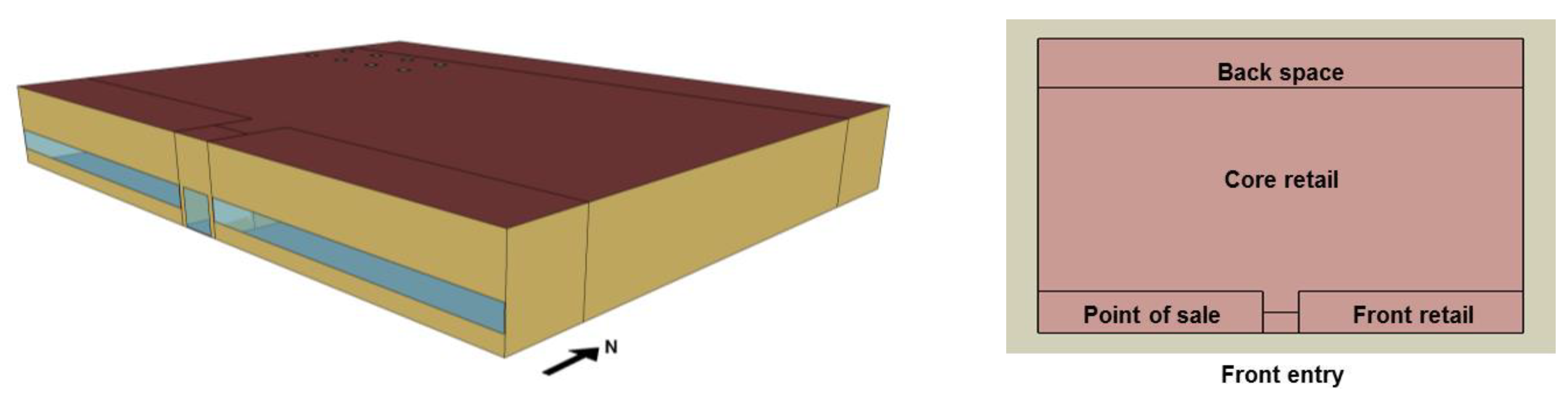
The present paper focuses on data from the SAR prototype buildings (Figure 1) [32], which are single-story structures with 2300 m² floor area, 7% window-to-wall ratio, and gas furnaces inside packaged air conditioning units. The HVAC is on from 7:00 a.m. to 9:00 p.m. on weekdays, from 7:00 a.m. to 10:00 p.m. on Saturdays, and from 9:00 a.m. to 7:00 p.m. on Sundays.

The main characteristics of this prototype are based on ASHRAE 90.1-2013 [21] and are listed in

Table 1. Modeling Specifications of Standalone Retail Building Prototype [18].

Characteristic	Description
Floor area (m2)	2300 (Length 54.3 m, width 42.4 m)
Floor to ceiling height (m)	6.1
Window-to-wall ratio (%)	7% overall, south wall 25.4%
Building Envelope
Walls	20.3 cm concrete masonry block + insulation per ASHRAE 90.1-2013 + 1.3 cm drywall
Roof	Roof membrane + insulation per ASHRAE 90.1-2013 + metal decking
Window U-factor and SHGC (Solar heat gain coefficient)	Varies with location as per ASHRAE 90.1-2013
Window operable area	2%
Foundation	15.2 cm concrete slab-on-grade + insulation per ASHRAE 90.1
Internal partition	1.3 cm gypsum board + 1.3 cm gypsum board
Internal thermal mass	15 cm standard wood
Air leakage rates (infiltration)	Peak: 0.2016 cfm/sf of above grade exterior wall surface area, adjusted by wind (when HVAC is off) Off Peak: 25% of peak infiltration rate (when HVAC is on) Additional infiltration through the building entrance
HVAC
Heating type	Gas furnace inside the packaged air conditioning unit
Cooling type	Packaged air conditioning unit
Distribution and terminal unit	Constant air volume air distribution 4 single-zone roof top units serving four thermal zones
Size	Autosized to design day
Efficiency	Based on climate location and design cooling/heating capacity and ASHRAE 90.1-2013 requirements
Thermostat setpoint (°C)	23.9 cooling/21.1 heating
Thermostat setback (°C)	29.4 cooling/15.6 heating
Ventilation	Per ASHRAE Standard 62.1-2013

. The designers of the prototype buildings assumed that the air leakage rate when the HVAC is on is 25% of the infiltration rate when the HVAC is off [12]. This approach was followed because EnergyPlus does not consider the detailed effects of the HVAC operation and wind direction on air leakage unless the airflow network model (ANM) is used. In general, the ANM is not used in most simulation models due to its complexity. In contrast, the online calculator utilizes CONTAM to estimate air leakage rates. Further building information such as lighting, occupancy, internal loads, and schedules are provided by Deru et al. [18]. The only difference between the base case and reduced air leakage cases in prototype building models was the air leakage rates, all other parameters were kept the same.

The present analyses of EnergyPlus simulation results focused on determining how improvements in airtightness in SAR buildings affected their main HVAC-related hourly and annual electricity and natural gas usage (i.e., cooling, heating, and fans). The results for hours when a building’s HVAC system was not in operation due to thermostat setback settings were not part of the analyses.

The EnergyPlus models with CONTAM-derived hourly infiltration rates were simulated for 52 US cities for the previously mentioned base case and the reduced infiltration rate cases. The 52 cities fall in one of the 16 climatic zones shown in

Table 2. Cities from climate zones 4–8 that were used to derive an equation for hourly heating energy savings as a function of outdoor temperature.

City	State	HDD65	CDD65	Climate Zone	City	State	HDD65	CDD65	Climate Zone
Baltimore	Maryland	4912	1133	4A	Syracuse	New York	7042	483	5A
Huntington	West Virginia	4496	998	4A	Boise	Idaho	6000	692	5B
Louisville	Kentucky	4440	1300	4A	Boulder	Colorado	6012	622	5B
Nashville	Tennessee	4032	1672	4A	Redmond	Oregon	6734	194	5B
New York City	New York	5090	1002	4A	Reno	Nevada	5768	384	5B
Richmond	Virginia	4087	1297	4A	Salt Lake City	Utah	5636	1054	5B
St. Louis	Missouri	5021	1437	4A	Spokane	Washington	6887	404	5B
Wichita	Kansas	4902	1585	4A	Bismarck	North Dakota	8686	408	6A
Albuquerque	New Mexico	4361	1210	4B	Burlington	Vermont	7903	407	6A
Portland	Oregon	4461	278	4C	Madison	Wisconsin	7504	520	6A
Seattle	Washington	4867	127	4C	Minneapolis	Minnesota	8002	634	6A
Boston	Massachusetts	5840	646	5A	Portland	Maine	7448	315	6A
Chicago	Illinois	6450	748	5A	Rapid City	South Dakota	7315	516	6A
Cleveland	Ohio	6108	617	5A	Traverse City	Michigan	7794	458	6A
Detroit	Michigan	6728	566	5A	Helena	Montana	7814	328	6B
Indianapolis	Indiana	5690	910	5A	Duluth	Minnesota	10213	140	7
Omaha	Nebraska	6052	1050	5A	Fairbanks	Alaska	14170	29	8
Pittsburgh	Pennsylvania	5986	684	5A

and the building envelope and other characteristics of the prototype buildings for that climate zones are already specified in the prototype buildings according to the building code requirements of the zone. However, the weather data, which includes temperature, relative humidly, solar radiation, wind speed and wind direction, used for simulations varied with the city. Regression models were developed to determine hourly energy savings. Energy use due to air leakage is primarily a function of the airflow rate, wind speed and indoor-to-outdoor air temperature differential. The airflow rate varies with indoor-to-outdoor pressure differentials that are mainly caused by wind, stack effect and HVAC operation. The temperature differential is primarily influenced by outdoor conditions given that HVAC setpoints are typically around 23 to 25 °C. Outdoor air temperature and wind speed were selected as the independent variables to be evaluated because they are likely the most influential and because they are readily available from the typical meteorological year database, which are sets of hourly data for specific locations that can be obtained from DOE [32]. The simulations were performed for all of the 52 cities using hourly weather data and the results were analyzed against the outdoor temperature and wind speed to investigate if there is a pattern that can be used to derive the simplified regression equations for predicting the energy savings due to air infiltration reduction in a commercial building.

The regression analyses focused on savings due to decreases in air leakage from 5.4 L/s/m² at 75 Pa (baseline) to 2 L/s/m² at 75 Pa (case 1). Case 1 was selected because it has a higher potential to be implemented throughout the United States than cases 2 and 3, given that it is the least stringent. Nevertheless, the analysis of case 1 serves as a proof of concept that could be applied to the other two scenarios and potentially to other building types. Additionally, a simplified approach was developed to estimate the annual percentage savings for cases 1, 2, and 3. The only input that users of this approach would need is the CZ in which the building is located. The models for energy savings and percentage savings were validated against results from the calculator.

3. Results and Discussions

The electricity and gas savings were calculated for the SAR buildings in 52 US cities using EnergyPlus models with CONTAM-derived hourly air leakage rates. The models were simulated using the hourly weather data for 52 cities listed in Table 2. The table only shows the heating degree days (HDD) and cooling degree days (CDD) as a heating/cooling geographical indicator for the cities and detailed meteorological data are obtained from the online weather depository [32]. As infiltration through the building envelope will impact HVAC energy use in the buildings, the analysis only included HVAC electricity and gas savings due to the considered reduced infiltration cases.

3.1. HVAC Energy Use

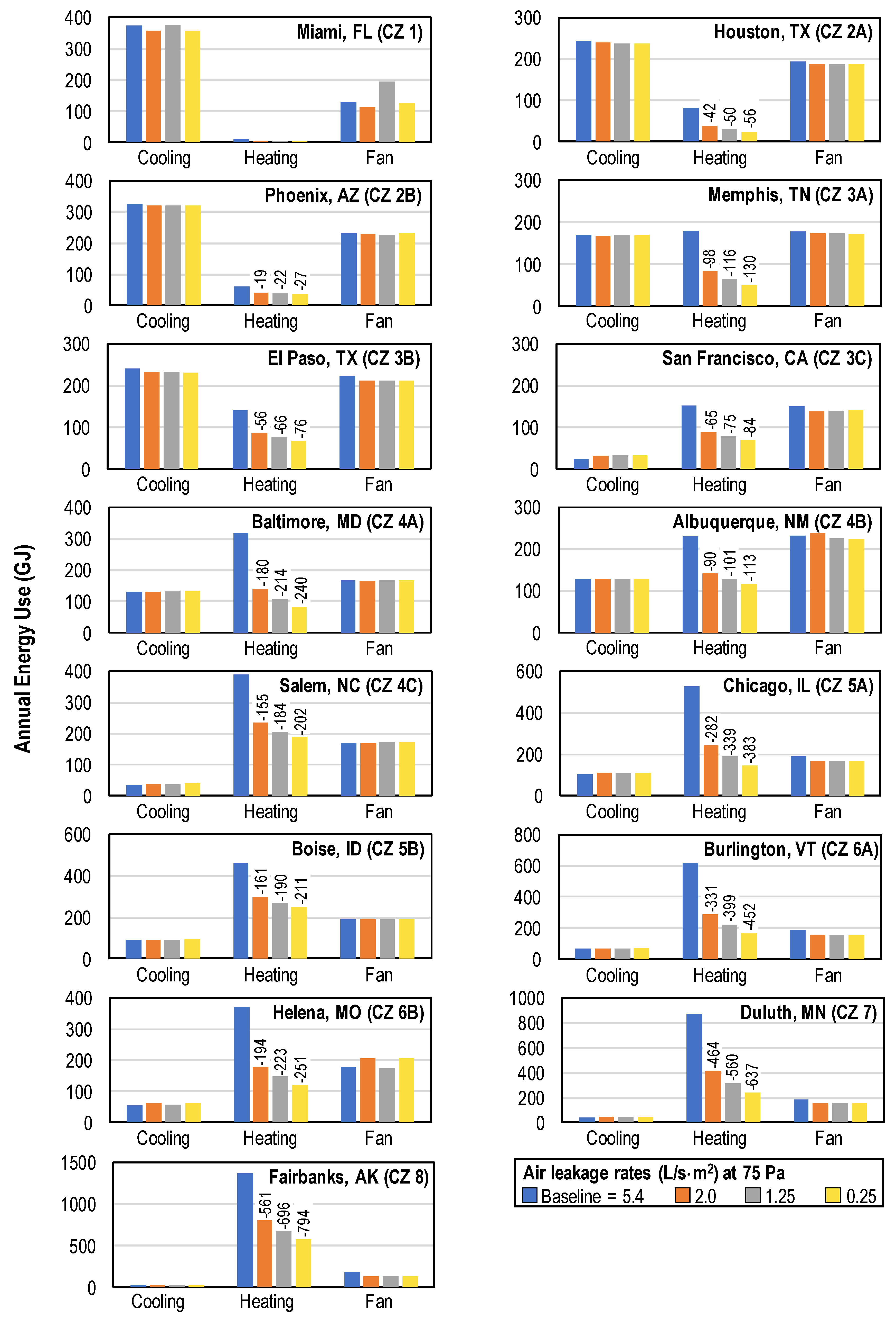
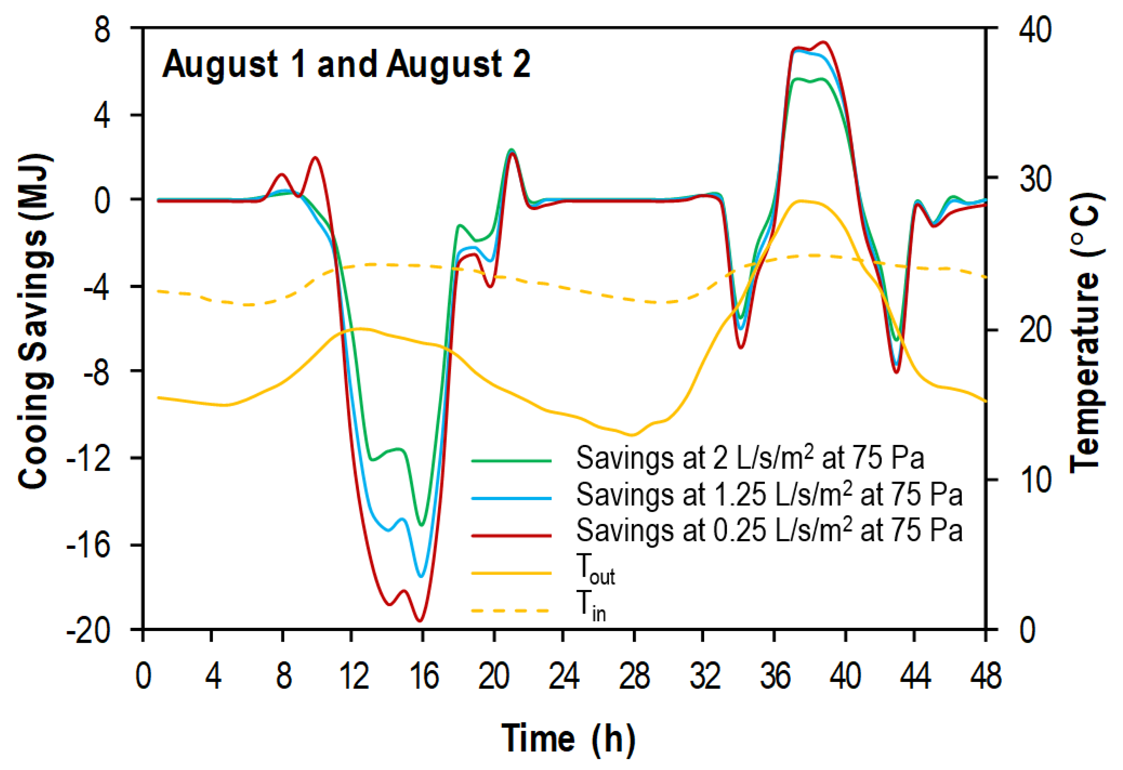
Figure 2 shows the annual HVAC energy use in the SAR buildings for the four assessed air leakage rates in 15 cities that are typically used to represent the DOE CZs. HVAC energy use is divided into its main components: cooling, heating, and fan. The results shown in Figure 2 suggest that reducing air leakage provides minimal decreases in cooling energy usage, even in cooling-dominated CZs, primarily because cooling loads in commercial buildings are generally governed by internal loads such as occupants, miscellaneous equipment, and lighting. In cities with relatively mild summers, cooling energy use increased with lower air leakage rates because in leaky buildings infiltration of outdoor air that was at a lower temperature than the indoor air lessened heat gains from internal loads. Figure 3 illustrates this phenomenon for San Francisco, California; cooling savings occur with increases in airtightness when the outdoor air temperature (T_out) is higher than the indoor temperature (T_in). However, the opposite is observed when T_out is lower than T_in.

Heating is provided in the SAR prototype with a gas furnace. Natural gas usage decreased in all cities with improvements in airtightness and the largest savings were observed in colder climates because these have a larger indoor-to-outdoor temperature differential. Lowering air leakage from 5.4 to 2 L/s/m² at 75 Pa in SAR buildings could lead to annual reductions in natural gas usage ranging from 5 GJ in Miami to 561 GJ in Fairbanks, Alaska. Further improvements to 0.25 L/s/m² at 75 Pa translated to annual savings of 6 GJ and 794 GJ, respectively, equivalent to decreases in heating energy of up to 58%. Although results for the SAR buildings indicate impressive decreases in heating energy usage with reductions in air leakage, Figure 2 indicates that there are diminishing returns as buildings get tighter.

Although air leakage had a significant effect on heating energy, these large savings were not reflected in fan usage. In general, fans consumed ~200 GJ per year regardless of CZ; thus, their contribution to total HVAC energy usage increased as the air leakage rate decreased. The consistency in fan energy usage may have resulted from the fact that SAR buildings use a constant-volume fan and constant outdoor air for ventilation while HVAC systems are operating.

3.2. HVAC Energy Savings

The following evaluations concentrate on heating energy savings because cooling energy was minimally influenced by the reduction in air leakage. CZs 1–3 were not studied because their heating loads are relatively low. The following analysis focused on energy savings due to improvements in energy savings in air leakage from 5.4 to 2 L/s/m² at 75 Pa. The annual analysis for each of the cities included 5278 hourly data points after deleting results for when the building’s HVAC system was not in operation due to thermostat setback settings.

3.2.1. Regression Equations for Hourly Energy Savings

The study explored the possibility of deriving an equation(s) that can predict hourly heating energy savings due to increased airtightness as a function of hourly outdoor temperature and/or wind speed. Such equations would enable a simple and convenient method to estimate energy savings using readily available weather data and without having to run a whole-building simulation model. Moreover, the equation(s) would not only be applicable to US buildings but also to regions around the world that meet the description of the DOE climate zones. Initial investigations focused on nine cities in CZs 4–8.

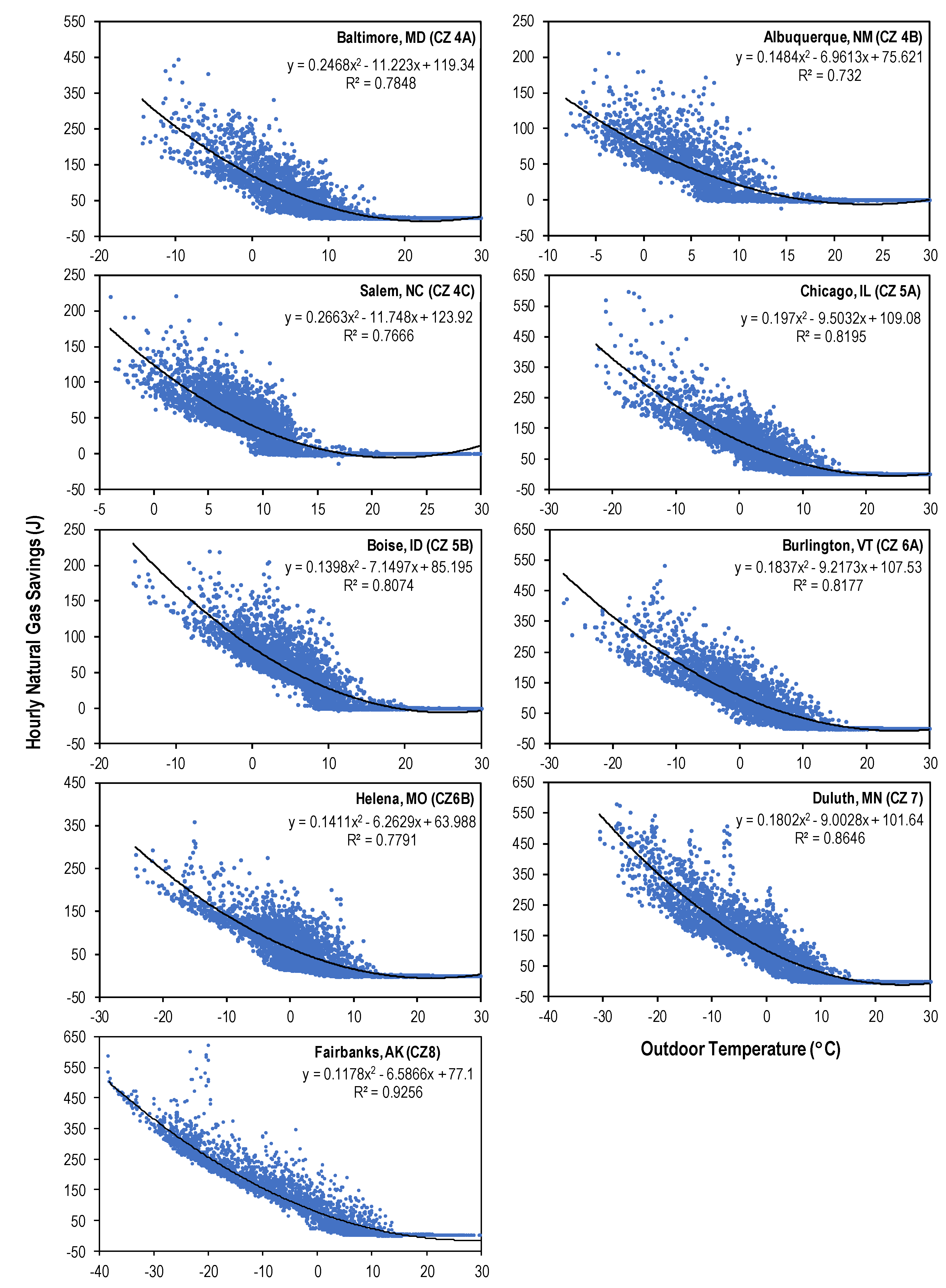
Numerous types of regression models were explored including various degrees of polynomials and exponential functions. Findings indicated that the 2nd degree polynomial tended to provide the best fit to the simulation results and that higher degree polynomials made minimal improvements. Figure 4 shows the hourly gas energy savings as a function of T_out, the derived models, and their coefficient of determination (R²). Cities in colder CZs showed stronger correlations (Fairbanks, Alaska: R² = 0.93) than warmer ones (Albuquerque, New Mexico: R² = 0.73). The derived equations were used to calculate annual energy savings for each of the nine cities. Results were within 0.1–2% of the values obtained using the calculator. A similar annual regression analysis was conducted for wind speed; however, the results suggested that there was a minimal correlation, if any, between wind speed and energy savings. This is likely because changes in wind speed are much smaller in magnitude and last for shorter periods of time than changes in outdoor air temperature. Similarly, adding incident solar radiation as an independent variable did not improve the correlation further. The reason might be that the effect of air leakage is a function of mass flow rate and the difference between indoor and outdoor temperatures. Solar radiation affects outdoor air temperature first; thus, so solar radiation is already indirectly accounted for. Thus, further assessments only considered T_out.

Given that the equations for the cities shown in Figure 4 provided encouraging results, the next step was to determine whether a single equation could be derived to predict heating energy savings for CZs 4–8 given that a single equation would be more convenient than having to use nine separate ones. To strengthen its validity, the combined equation would need to be tested with multiple cities that are in different CZs. To this end, data from the 35 cities listed in Table 2 were combined.

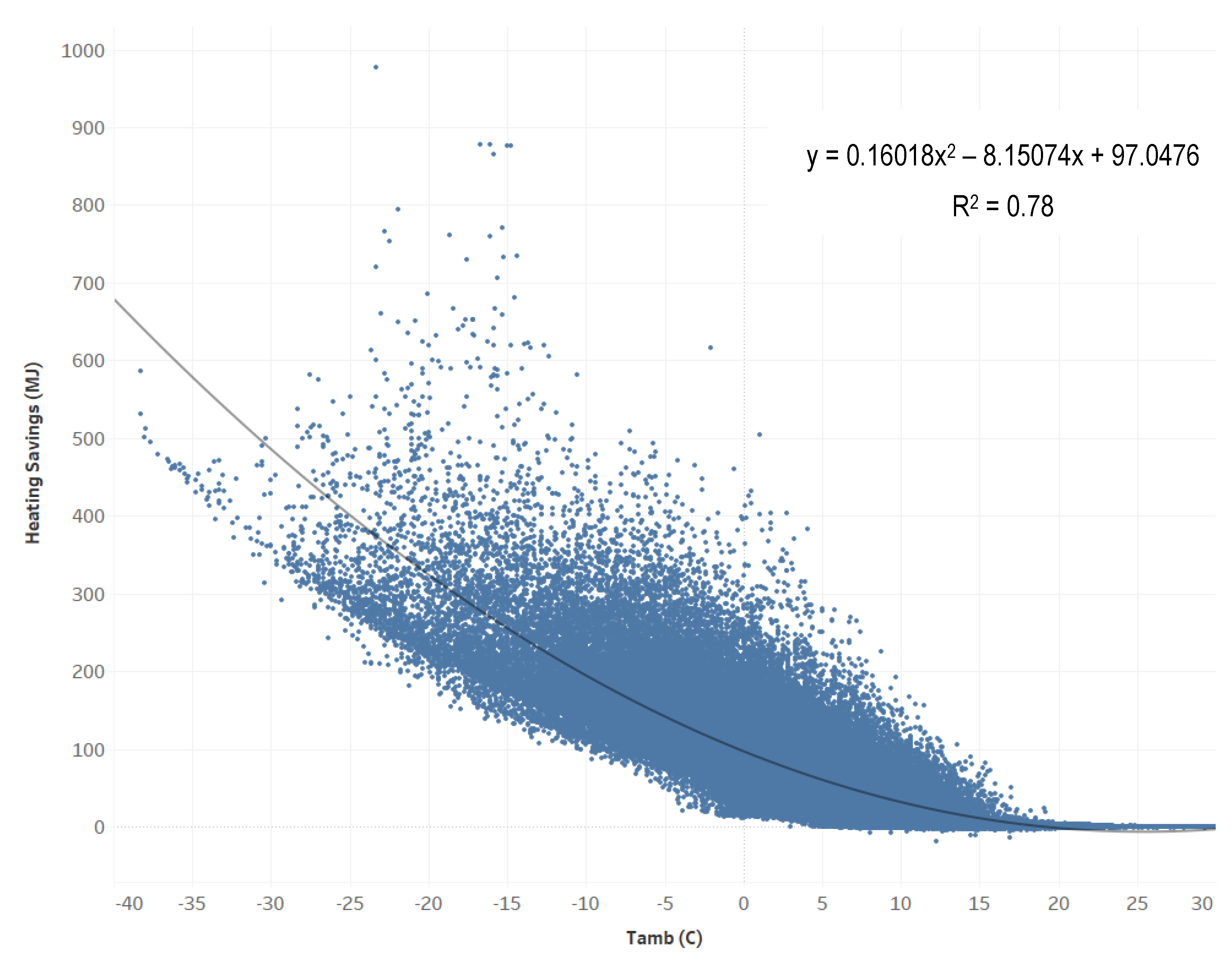
Figure 5 shows that natural gas savings and T_out were relatively well correlated (R² = 0.78) considering the fact that data from multiple cities with quite different weather conditions were combined. However, when the derived equation was used to calculate the annual heating savings of each of the cities in Table 2 as a function of their corresponding outdoor temperatures, results differed from those obtained using the calculator by more than 30% in 10 of the cities, indicating that the derived model was not adequate. These large discrepancies are due to the fact that although cities in different CZs may experience similar outdoor temperatures, variations in other outdoor parameters (e.g., solar radiation and relative humidity) will influence the heating energy loads and thus the savings that can be obtained through improvements in airtightness.

Subsequent investigations determined what CZs could be grouped to derive heating energy savings models while minimizing discrepancies with results from the calculator.

Table 3. Models for hourly heating energy savings in climate zones 4–8, annual heating energy savings results for representative cities, and percent error from comparison to values from the calculator.

Climate Zones	# Grouped Cities	Equation for Annual Heating Savings (MJ)	Range in % Difference *	Cities That Are Representative of DOE’s Climate Zones
				City	Climate Zone	Annual Heating Savings (MJ)
						Calculator	Derived Equation	% Difference *
4A, 5A, 6A, 7	28	0.170058 × Tout2 −9.07279 × Tout + 106.422	−13 to +24%	Baltimore	4A	179,395	165,188	8%
				Salem	4C	155,385	147,285	5%
				Chicago	5A	282,496	270,453	4%
				Burlington	6A	331,241	325,008	2%
				Duluth	7	463,511	480,714	−4%
4B, 5B	7	0.11496 × Tout2 −6.55559 × Tout + 79.8516	−17 to +18%	Albuquerque	4B	90,577	103,153	−14%
				Boise	5B	161,177	149,828	7%
6B	1	0.141061 × Tout2 −6.26294 × Tout + 63.9883	0.02%	Helena	6B	193,853	193,896	0%
8	1	0.11178 × Tout2 −6.58669 × Tout + 77.1	0.003%	Fairbanks	8	561,260	561,241	0%

* The % difference was calculated with respect to the annual heating savings from the calculator. Positive values indicate that the model underpredicted annual savings. Negative values indicate that the model overpredicted the annual savings. T_out is the outdoor air temperature.

lists the grouped CZs and the percent difference between annual savings that were estimated using the derived equations and the calculator. The savings equation for CZs 4A, 5A, 6A, and 7 was obtained by combining data from 28 cities. Percent errors resulting from the savings equation ranged from −13% to 24%; positive values indicate that the model underpredicted annual savings, and negative values indicate the model overpredicted annual savings. The large percent error span likely resulted from combining data from cities with quite different outdoor conditions. Nevertheless, 8 of the 28 cities had savings with percent differences of less than 10%. The model for CZs 4B and 5B grouped data from seven cities, and the derived model had percent differences that ranged from −17% to 18%. Equations for CZs 6B and 8 were derived using data from one city because the developers of the calculator decided to invest fewer resources to generate EnergyPlus and CONTAM models in CZs with low populations. Fewer cities lead to lower variability in the outdoor temperature; thus, the annual savings percent difference was less 0.02%. Table 3 also shows the annual heating savings that were obtained using the derived models and the calculator for cities that DOE uses as representative of each of the CZs. Results show a maximum discrepancy of −14%.

3.2.2. Annual Relative Heating Savings after Improvements in Airtightness

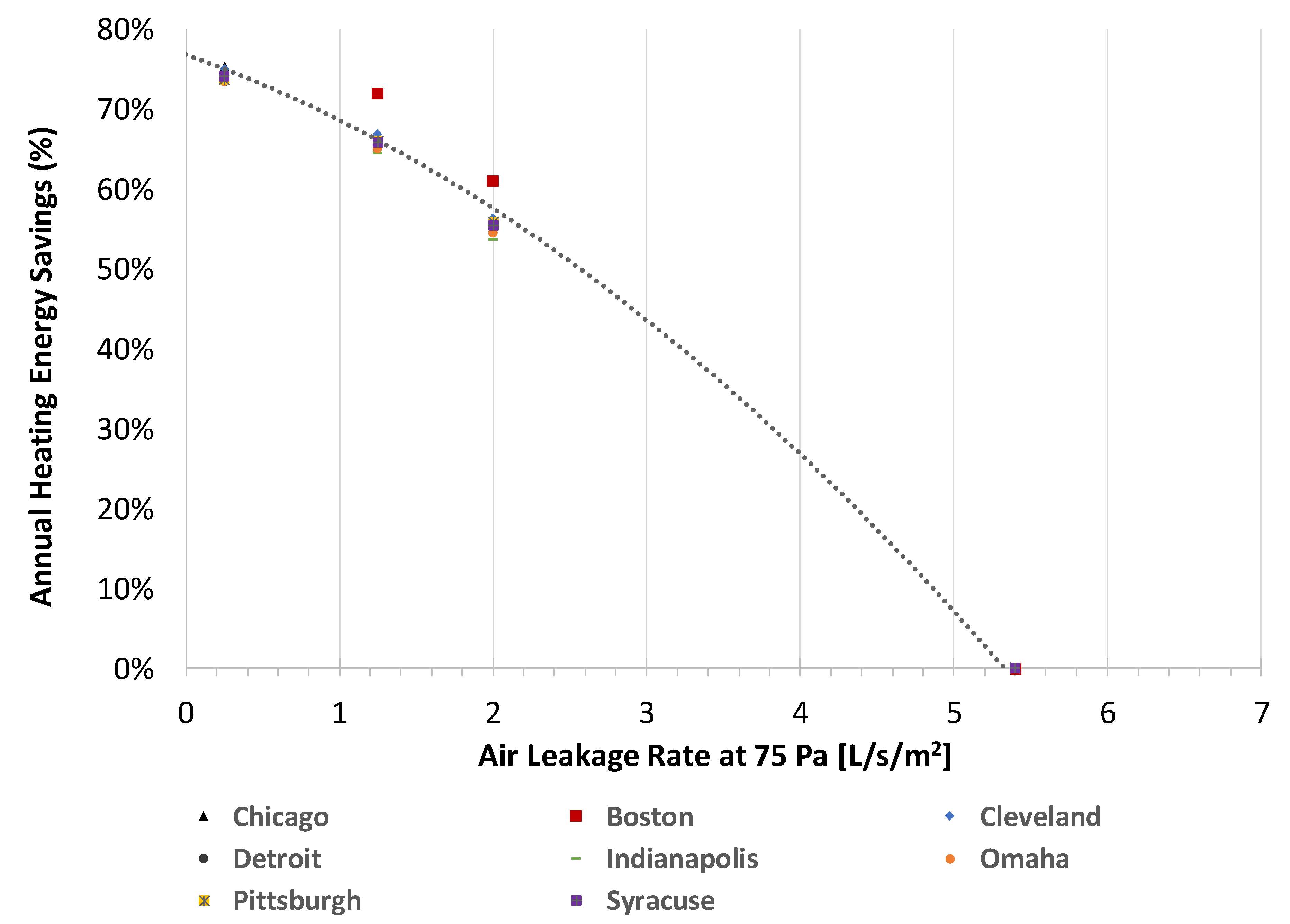
Investigations were also conducted to determine whether models could be generated to estimate the annual relative or percent heating energy savings as air leakage rates decrease. These models could allow building owners and designers to determine target leakage rates when retrofitting a building envelope. Calculations of the percent energy savings for cases 1, 2, and 3 with respect to the baseline revealed distinct patterns that could be used to predict energy savings for CZs 4–8. For example, Figure 6 shows the relative energy savings for SAR buildings in CZ 5A; results indicate that the annual percent savings for the eight cities in this CZ are similar (~75%) in buildings that reduce air leakage from 5.4 L/s/m² at 75 Pa (pre-retrofit) to 2 L/s/m² at 75 Pa (post-retrofit). Similar patterns were observed when post-retrofit leakage rates of 1.25 L/s/m² and 0.25 L/s/m² at 75 Pa were examined; findings suggest that buildings in the eight cities achieve savings of 66% and 55%, respectively. The only apparent outlier was Boston, where the gas energy savings were slightly higher (72% and 61%, respectively) than what was observed among the other cities.

As a clear trend is seen in Figure 6, a regression line for annual relative gas energy savings can be expressed as

$$\mathrm{Savings}(\%)=f(Q_{post})=-\mathrm{A}·Q_{post}^2 -\mathrm{B}·Q_{post}+\mathrm{C}$$

(1)

where Q_post represents the air leakage rates after the retrofit (post-retrofit) in L/s/m² at 75 Pa, and A, B, and C are constants that vary with the CZ or grouped CZs being evaluated. For example, for the simulated gas energy savings in CZ 5A, Equation (1) becomes:

$$\mathrm{Savings}(\%)=-0.0117·Q_{post}^2-0.088·Q_{post}+0.7736$$

(2)

Note that Equation (1) can only be used if the baseline is 5.4 L/s/m² at 75 Pa (pre-retrofit), as all the energy savings were calculated with respect to this baseline. To predict energy savings from any arbitrary pre-retrofit infiltration rates, Equation (1) needs to be adjusted to these pre-retrofit conditions. Equation (3) shows how such adjustments are accounted for and thus allows for the prediction of gas energy savings from and to arbitrary air leakage rates.

$$\mathrm{Savings}(\%)=\frac{f\left(Q_{post}\right)-f\left(Q_{pre}\right)}{1-f\left(Q_{pre}\right)}$$

(3)

Q_pre is the air leakage rate (pre-retrofit) for gas energy savings prediction. The two terms in the numerator represent the difference in energy savings from existing conditions Q_pre (baseline) to a new air leakage rate Q_post. The two terms in the denominator are used to adjust the equation to be valid for any arbitrary pre-retrofit conditions.

From Equations (1) and (3), the following generalized equation was derived for the annual relative energy savings in each of the CZs:

$$\mathrm{Savings}(\%)=\frac{\mathrm{A}\left(Q_{pre}^2-Q_{post}^2\right)+\mathrm{B}\left(Q_{pre}-Q_{post}\right)}{1+\mathrm{A}\left(Q_{pre}^2\right)+\mathrm{B}\left(Q_{pre}\right)-\mathrm{C}}$$

(4)

where Q_pre and Q_post are the air leakage rates before and after the retrofit in L/s/m² at 75 Pa, and A, B, and C are constants that vary with the CZ or with grouped CZs being evaluated. The generalization of the equation makes it independent of the baseline air leakage rate. As long as the pre-retrofit infiltration and post-retrofit infiltration rates are known, the equation can be used to calculate the annual heating energy savings without any simulations or equations.

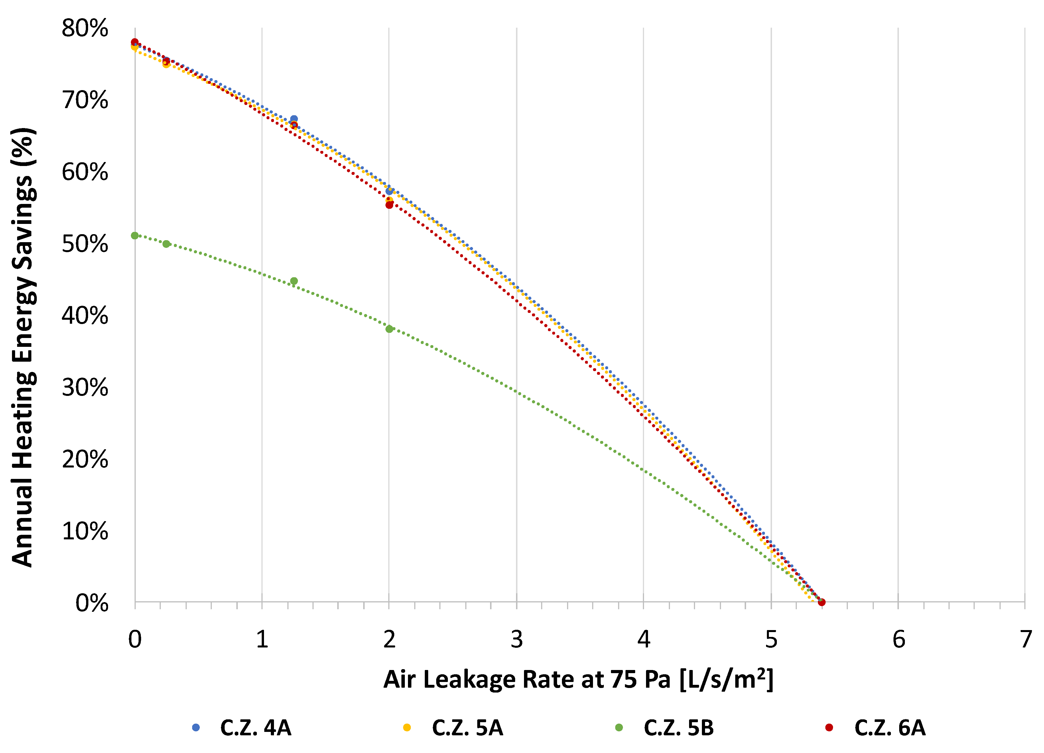
Figure 7 illustrates the derived percent savings models for each of these CZs and shows that the results 4A, 5A, and 6Az are similar, implying that these could share a single model. Similar observations were made with the models for CZs 4B and 5B.

Table 4. Constants to calculate the annual relative heating energy savings using Equation (4) in climate zones 4–8, and annual relative heating energy savings results for representative cities using 5.4 L/s/m² as the pre-retrofit air leakage rate.

Climate Zones	Number of Cities	Predicted Energy Savings Using Equation (4)	Range in % Difference *	Cities That Are Representative of DOE’s Climate Zones
				City	Climate Zone	Annual Heating Energy Savings Qpre = 5.4 L/s/m2 at 75 Pa
						Qpost = 2.0 L/s/m2 at 75 Pa	Qpost = 1.25 L/s/m2 at 75 Pa	Qpost = 0.25 L/s/m2 at 75 Pa
4A, 5A, 6A	23	A = 0.0117, B = 0.0806, C = 0.7767	−6.4%–5.9%	Baltimore	4A	58%	68%	77%
				Chicago	5A	56%	67%	75%
				Burlington	6A	57%	67%	76%
4B, 5B	7	A = 0.0091, B = 0.0457, C = 0.5127	−2.3%–2.3%	Albuquerque	4B	41%	46%	52%
				Boise	5B	37%	43%	48%
6B	1	A = 0.0138, B = 0.0575, C = 0.713	-	Helena	6B	54%	62%	70%
7	1	A = 0.0115, B = 0.0843, C = 0.790	-	Duluth	7	57%	68%	76%
8	1	A = 0.0084, B = 0.0794, C = 0.6727	-	Fairbanks	8	47%	57%	65%

* The % difference was calculated with respect to annual heating savings from the calculator. Positive values indicate that the model underpredicted the annual savings. Negative values indicate that the model overpredicted the annual savings.

lists the cities for the models that combine CZs, as well as for CZs 6B, 7, and 8. Additionally, Table 4 includes annual relative heating energy savings results for representative cities using 5.4 L/s/m² as the pre-retrofit air leakage rate.

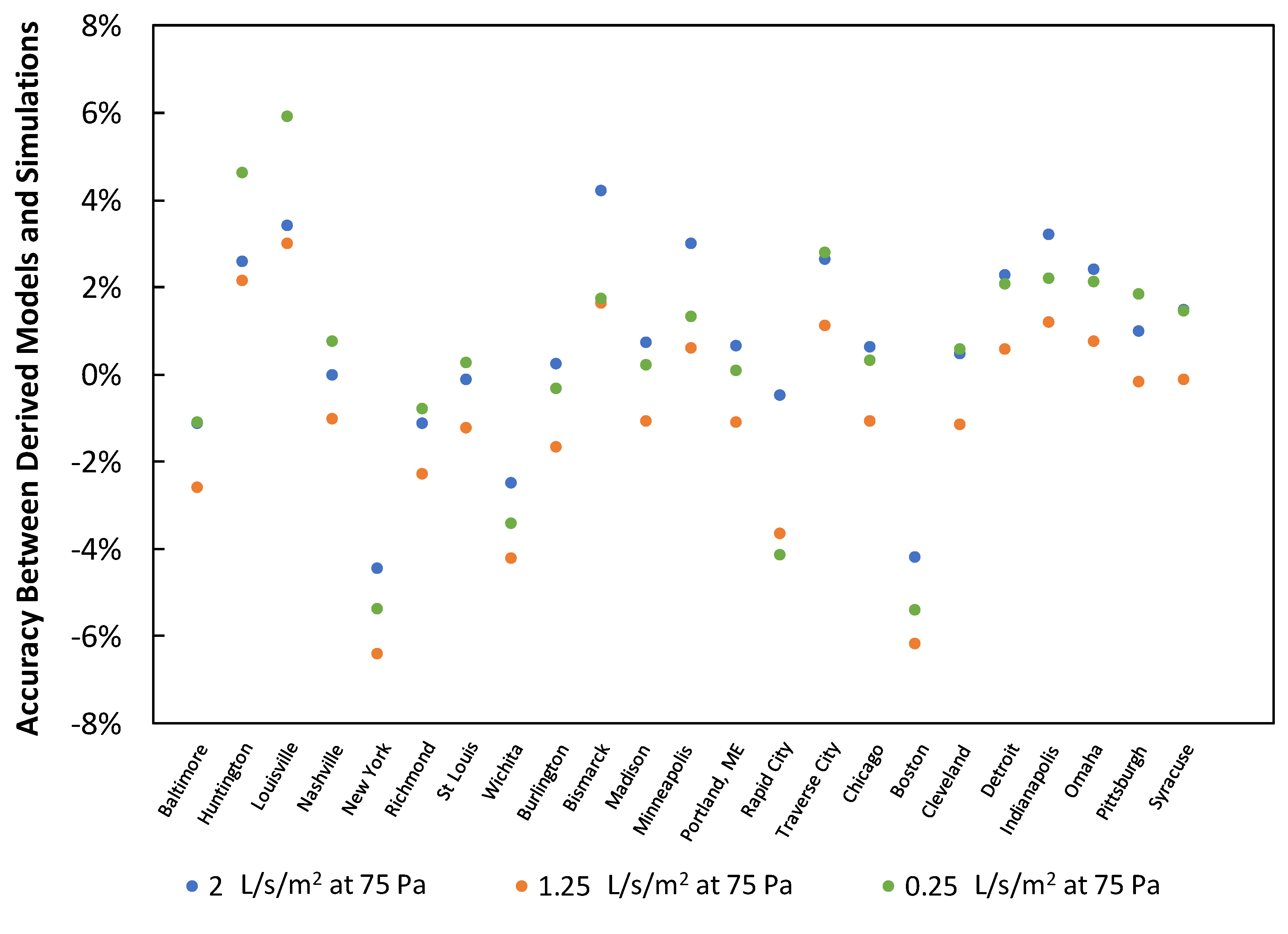
Figure 8 shows that the annual savings results from the combined model for CZs 4A, 5A, and 6A are ±6% different from the results obtained using the calculator. Note that the results were not normalized for the floor area of the building.

3.3. Limitations and the Next Steps

The methodology described in this paper was developed as a concept for a simplified approach to estimate the energy savings due to improvements in airtightness. Although results for the stand-alone prototype building appear to be promising, the models could be improved by adding data from more cities to the regression analysis. The analysis is based on the building area and other characteristics of prototype standalone retail building and three different air infiltration rate reductions. This study can further be extended to normalize results by including other building characteristics such as building area, floor height, window to wall ratio etc. and additional sets of infiltration rate reductions. The validation of the proposed methodologies was performed by comparing results from the derived equations and the online calculator. Even though the results show good agreement, comparison of energy savings results with data from actual buildings would add a great value. Future work includes further validating the methodology by following the proposed approach with data from other prototype buildings. Files for EnergyPlus models with CONTAM-derived hourly infiltration rates are readily available for medium offices and mid-rise apartments, hotel, hospital and may soon be available other prototype buildings. Although, conducting field validations with pre- and post-retrofit infiltration rates and heating energy consumption would add confidence to the proposed methodology, given the large number of potential variations in a single building type, the DOE prototype buildings are primarily intended to serve as a standardized source for comparative results. That is, it could be inferred that an estimated 30% energy savings in a stand-alone prototype retail building could lead to similar savings in an actual SAR building.

4. Conclusions

Simplified approaches were developed to estimate hourly and annual heating energy savings and annual percent energy savings due to improvements in airtightness in the DOE standalone retail prototype building. The equations that predict energy savings only require readily available hourly outdoor temperature data for the city where the building is located. Annual energy savings that were estimated using the proposed approach and the online calculator differed by 15% to 24%. Using more cities to generate the models could reduce this difference even further. The equations that predict percent energy savings for retrofitted buildings only require their expected pre- and post-retrofit air leakage rates. Results indicate that estimated percent energy savings were within 5% of the values obtained through the calculator. Both of the developed approaches expand the ability of building owners and designers to make educated decisions on improvements in airtightness beyond the 52 US cities that are covered by the calculator without the need to generate a whole-building simulation model. Moreover, hourly energy savings results give users the flexibility to isolate specific periods of interest. Future research could include improving the simplified method by adding data from more cities and conducting field assessments to validate the results, as well as developing similar methods for other prototype buildings. In the future, this analysis could be extended to cover more air infiltration reduction rates and more building types to develop potential generalized equations that can be normalized based on the building type, area, and infiltration rate reductions.

References

- US Department of Energy. Windows and Building Envelope Research and Development: Roadmap for Emerging Technologies. 2014. Available online: https://www.energy.gov/sites/prod/files/2014/02/f8/BTO_windows_and_envelope_report_3.pdf (accessed on 20 August 2018).
- Cui, S.; Cohen, M.; Stabat, P.; Marchio, D. CO2 tracer gas concentration decay method for measuring air exchange rate. Build. Environ. 2015, 84, 162–169. [Google Scholar] [CrossRef]
- Kim, M.; Jo, J.; Jeong, J. Feasibility of building envelope air leakage measurement using combination of air-handler and blower door. Energy Build. 2013, 62, 436–441. [Google Scholar] [CrossRef]
- Liu, W.; Zhao, X.; Chen, Q. A novel method for measuring air infiltration rate in buildings. Energy Build. 2018, 168, 309–318. [Google Scholar] [CrossRef]
- Hong, G.; Kim, B.S. Field measurements of infiltration rate in high residential buildings using the constant concentration method. Build. Environ. 2018, 97, 48–54. [Google Scholar] [CrossRef]
- American Society for Testing and Materials. ASTM E799-10: Standard Test Method for Determining Air Leakage Rate by Fan Pressurization; ASTM: West Conshohocken, PA, USA, 2010. [Google Scholar]
- Brennan, T.; Anis, W.; Nelson, G.; Olson, C. ASHRAE 1478: Measuring airtightness of mid- and high-rise non-residential buildings. In Proceedings of the Thermal Performance of the Exterior Envelopes of Whole Buildings—12th International Conference, Clearwater, FL, USA, 1–5 December 2013. [Google Scholar]
- Zhivov, A.; Herron, D.; Durston, J.L.; Heron, M.; Lea, G. Air tightness in new and retrofitted US Army buildings. Int. J. Vent. 2014, 12, 317–330. [Google Scholar] [CrossRef]
- Jones, D.; Brown, B.; Thompson, T.; Finch, G. Building enclosure airtightness testing in Washington State–Lessons learned about air barrier systems and large building testing procedures. In Proceedings of the ASHRAE 2014 Annual Conference, Seattle, WA, USA, 28 June–2 July 2014. [Google Scholar]
- Ricketts, R. Impact of large building airtightness requirements. In Proceedings of the Thermal Performance of the Exterior Envelopes of Whole Buildings—13th International Conference, Clearwater, FL, USA, 4–8 December 2016. [Google Scholar]
- Crawley, D.B.; Hand, J.W.; Kummert, M.; Griffith, B.T. Contrasting the capabilities of building energy performance simulation programs. Build. Environ. 2008, 43, 661–673. [Google Scholar] [CrossRef] [Green Version]
- Gowri, K.; Winiarski, D.; Jarnagin, R. Infiltration Modeling Guidelines for Commercial Building Energy Analysis; Technical Report No. PNNL-18898; Pacific Northwest National Laboratory: Richland, WA, USA, 2009. [Google Scholar]
- Ng, L.C.; Musser, A.; Persily, A.K.; Emmerich, S.J. Multizone airflow models for calculating infiltration rates in commercial reference buildings. Energy Build. 2013, 58, 11–18. [Google Scholar] [CrossRef]
- Han, G.; Srebric, J.; Enache-Pommer, E. Different modeling strategies of infiltration rates for an office building to improve accuracy of building energy simulations. Energy Build. 2015, 86, 288–295. [Google Scholar] [CrossRef]
- Emmerich, S.; Persily, A.; McDowell, T.P. Impact of commercial building infiltration on heating and cooling loads in U.S. office buildings. Presented at 26th AIVC Conference, Brussels, Belgium, 21–23 September 2005. [Google Scholar]
- Emmerich, S.; Persily, A. Analysis of US commercial building envelope air leakage database to support sustainable building design. Int. J. Vent. 2014, 12, 331–344. [Google Scholar] [CrossRef]
- Shrestha, S.; Hun, D.; Ng, L.; Desjarlais, A.; Emmerich, S.; Dalgleish, L. Online airtightness savings calculator for commercial buildings in the United States, Canada, and China. In Proceedings of the Thermal Performance of the Exterior Envelopes of Whole Buildings—13th International Conference, Clearwater, FL, USA, 4–8 December 2016. [Google Scholar]
- Deru, M.; Field, K.; Studer, D.; Benne, K.; Griffith, B.; Torcellini, P.; Halverson, M.; Winiarski, D.; Liu, B.; Rosenberg, M.; et al. DOE Commercial Reference Building Models for Energy Simulation–Technical Report; National Renewable Energy Laboratory: Golden, CO, USA, 2010. [Google Scholar]
- Goel, S.; Athalye, R.; Wang, W.; Zhang, J.; Rosenberg, M.; Xie, Y.; Hart, R.; Mendon, V. Enhancements to ASHRAE Standard 90.1 Prototype Building Models; Technical Report No. PNNL-23269; PNNL: Richland, WA, USA, 2014. [Google Scholar]
- Department of Energy (DOE). Commercial Prototype Building Models. 2016. Available online: https://www.energycodes.gov/commercial-prototype-building-models (accessed on 5 November 2018).
- American Society of Heating, Refrigerating and Air-Conditioning Engineers. Energy Standard for Buildings Except Low Rise Residential Buildings; ANSI/ASHRAE/IES Standard 90.1-2013; ASHRAE: Atlanta, GA, USA, 2013.
- Department of Energy (DOE). Auxiliary EnergyPlus Programs–Extra Programs for EnergyPlus; DOE: Washington, DC, USA, 2016.
- Dols, W.S.; Polidoro, B. CONTAM User Guide and Program Documentation; Technical Note 1887; National Institute of Standards and Technology: Gaithersburg, MD, USA, 2015. [Google Scholar]
- Ng, L.C.; Ojeda Quiles, N.; Dols, W.S.; Emmerich, S.J. 2018, Weather correlations to calculate infiltration rates for U. S. commercial building energy models. Build. Environ. 2005, 127, 47–57. [Google Scholar] [CrossRef] [PubMed]
- Jarnagin, R.E.; Bandyopadhyay, G.K. Weighting Factors for the Commercial Building Prototypes Used in the Development of ANSI/ASHRAE/IENSA Standard 90.1-2010; Technical Report No. PNNL-19116; PNNL: Richland, WA, USA, 2010. [Google Scholar]
- U.S. Energy Information Administration. Commercial Buildings Energy Consumption Survey. 2012. Available online: https://www.eia.gov/consumption/commercial/ (accessed on 20 August 2018).
- Briggs, R.S.; Lucas, R.G.; Taylor, T. Climate classification for building energy codes and standards: Part 2–Zone definitions, maps and comparisons. ASHRAE Trans. 2003, 109, 122–130. [Google Scholar]
- Emmerich, S.J.; McDowell, T.P.; Anis, W. Investigation of the Impact of Commercial Building Envelope Airtightness on HVAC Energy Use; NISTIR 7238; NIST: Gaithersburg, MD, USA, 2005. [Google Scholar]
- International Code Council, Inc. International Energy Conservation Code; ICC: Washington, DC, USA, 2015. [Google Scholar]
- US Army Corps of Engineers. Air Leakage Test Protocol for Building Envelopes. 2012. Available online: https://www.aikencolon.com/assets/images/pdfs/retrotec/USACE-ASTM-E-779-Air-Leakage-Test-Protocol.pdf (accessed on 20 August 2018).
- US Department of Energy (US DOE). Weather data by Region, All Regions—North and Central America WMO Region 4. 2018. Available online: https://energyplus.net/weather-region/north_and_central_america_wmo_region_4/USA%20%20 (accessed on September 2018).
- US Department of Energy. 90.1 Prototype Building Models Sand Alone Retail. Available online: https://www.energycodes.gov/901-prototype-building-models-stand-alone-retail (accessed on September 2018).
Figure 1.
Standalone retail building prototype. Left: Building shape and orientation. Right: Layout of five thermal zones [18].
Figure 2.
Annual HVAC energy usage in the stand-alone retail prototype buildings for the four assessed air leakage rates in 15 cities representative of DOE’s climate zones. Numbers above bars indicate the difference in energy use with respect to the baseline.
Figure 3.
Hourly cooling energy savings at various airtightness levels for the stand-alone retail prototype building in San Francisco, California.
Figure 4.
Correlation between outdoor air temperature and heating energy savings in nine cities representative of climate zones 4–8.
Figure 5.
Heating savings as a function of outdoor temperature for the combined 35 cities in climate zones 4 and 8 that are listed in Table 1.
Figure 6.
Annual relative heating energy savings due to increased airtightness in stand-alone retail prototype buildings in Climate zone 5A. The baseline leakage rate is 5.4 L/s/m2.
Figure 7.
Results from models that calculate the annual relative heating energy savings with increased airtightness in stand-alone retail prototype buildings in climate zones 4A, 5A, 5B, and 6B using Equation (1) and constant values in Table 3.
Figure 8.
Differences between annual relative heating savings from the calculator and the predicted savings using the derived equation (Equation (4)) for climate zones 4A, 5A, and 6A.