Benefits of a Demand Response Exchange Participating in Existing Bulk-Power Markets †


Department of Electrical Engineering and Computer Science, South Dakota State University, Brookings, SD 57007, USA
*
Author to whom correspondence should be addressed.
†
This manuscript is greatly expanded and improved on one of our previous conference publications titled “A Framework for Integrating Demand Response Into Bulk-Power Markets”.
Energies 2018, 11(12), 3361; https://doi.org/10.3390/en11123361
Submission received: 1 November 2018
/
Revised: 20 November 2018
/
Accepted: 20 November 2018
/
Published: 1 December 2018
(This article belongs to the Special Issue Demand Response in Electricity Markets)
Abstract
:In most U.S. market sponsored demand response (DR) programs, revenue earned from energy markets has been relatively low compared to DR used for capacity markets and ancillary services. This paper presents an aggregated DR model participating in the bulk-power market as a service through a pool-based entity called demand response exchange (DRX). Using the DRX structure, DR providers can participate in energy markets as a service to benefit bulk-power market entities. The benefits and challenges to each market entity using DR-as-a-service are presented in an extended review. The DRX model in this study is a market entity that operates with the day-ahead market to select DR offers that minimize electric utility payments. A case study was performed using the proposed DRX model on the IEEE 24-bus system, augmented to represent actual bulk-power market prices to study factors that influence utility payments under the DRX-market paradigm. Two high-price days of the PJM market were simulated, and it was shown for a single day on the augmented test case that spending $69,955 for DR-as-a-service results in a reduction of utility payments of $864,199. The day-ahead generator supply curve, network congestion, and DR curtailment were found to be the most influencing factors that impact the benefit of using DR-as-a-service.
1. Introduction
The U.S. Federal Energy Regulatory Commission (FERC) issued Order No. 888 to deregulate the U.S. electric power system [1], which granted open access of transmission to all generators. The forethought of deregulation was to encourage investments to provide cheaper electric power generation by competing independent power producers. Under deregulation, increasing electric demand, combined with the physical constraints of the electric power network, can give unlimited market power to a few generators, resulting in relatively large locational marginal prices (LMP). These generators are typically fossil-fueled generators that have a fast start and ramp time.
In such cases of LMP spikes, demand response (DR) can be used to intentionally change normal power consumption in response to the electricity price (LMPs), or in exchange for financial incentives [2]. Technical and economic benefits of DR have been identified by law makers [2] and the research community [3]. Across the literature, the most common advantages of DR are:
The literature broadly classifies DR programs into two categories: (a) price-based (PBDR), and (b) incentive-based (IBDR) [3]. Under PBDR, customers are exposed to time-varying rates to which they are expected to adapt their demand. PBDR is administered by the electricity retailers or LSEs, and the participants are mostly residential and small commercial organizations. Among the two classes of DR, PBDR has a smaller contribution (∼7% in 2010) [11], but this number is increasing in the past decade as more utilities are offering dynamic pricing, and customers have gained access to advanced metering [12].
As per the latest report period, IBDR has greater enrollment than PBDR [12]. Under IBDR, customers are paid incentives for modifying their demand during requested time periods [3]. While both classes of DR have their own advantages and impediments, some of the challenges are as follows [13]:
- price volatility is increased using real-time pricing (RTP) [14];
- additional investment is required for advanced metering to communicate RTP to customers [15];
- RTP requires customers’ prompt response in consumption to reduce billing [16]; and
- a new peak may be formed during off-peak hours, commonly known as the rebound-effect [17].
The main source of revenue in PBDR comes from the energy market, as the demand is modified in response to the price of retail electric energy [18]. FERC Order No. 719 was issued to allow non-generating resources to participate in the bulk-power market, which enabled entities to bid load reduction directly into the electricity market [19]. Bidding load reductions are only possible with IBDR, where the response is determined by the difference between the customer baseline (CBL) and the actual electricity consumption. With the capability to participate in the organized power market, IBDR can generate revenue from capacity, energy, and ancillary markets [11]. The ability to control loads in IBDR generates interest among the power research community, as the impact of load variation on the power system can be studied [20,21]. There are a growing number of power system researchers that consider IBDR as an effective solution to increase economic efficiency [14,22]. Increased sustainability in electric power systems is also commonly listed as a benefit of DR; in [10], the authors describe the economic and environmental sustainability of an IBDR in a smart grid. In this paper, we use a pool-based IBDR model to reduce utility payments, improving the economic efficiency of the system.
As IBDR provides the opportunity to control loads, regulatory bodies (FERC Order No. 745) provided opportunity to participate in the market as a resource [23]. Some early work was conducted to study the impact of DR participating in the energy market [24,25], where DR was modeled as a price responsive load to maximize social welfare. Because the demand is elastic to price, the load shifted to a lower price point to minimize system operation cost. The DR exchange (DRX) is a conceptual pool-based market to trade DR offers [26]. DRX provides the power system operator and other market entities with additional flexibility [26]. There has been increasing interest in DRX-based DR because of the flexibility in modeling the objective function, and the ability to maximize the social welfare of the DR provider and other market entities. There has been considerable research in forming market clearing mechanisms for DRX with various objective functions [27,28,29]. In this work, we implement the DRX for minimizing electric utility payments. The DR providers are paid by utilities for the service, as the utility is benefited via reduced LMPs and lower payments. The DRX model in this work ensures that the rebound-effect does not significantly increase utility payments during off-peak hours.
Residential resource optimization to maximize profit of DR aggregators (DRA) participating in a bulk-power market through a DRX is presented in [30], but there was no model presented to integrate DRX into existing electricity markets. The authors in [31] propose a market clearing algorithm for DR offers, and illustrate the proposed technique on a test system. Though the paper provides a market clearing technique, there is no evidence of interaction with a bulk-power market, and market entity surplus is not included. In [28], a DRX is presented that operates in the day-ahead, intra-day, and balancing markets, where wind power plants participate in DRX to maximize their profit. The paper mainly quantifies the DR-market interaction to maximize the profit of the wind power plant, but the interaction of bulk-power entities and surplus is missing. A similarly themed research publication can be found in [29], where the DRX is used by virtual power plants to maximize their profits. The work presented in [32] describes DR bid/offer modeling based on CBL attributes. This is a significant work in this field, as customer willingness/behavior is important in determining the cost of DR. However, a market model was not considered for the ISO–DRX interaction. One aspect of DRX-related research that has not been well-studied is models for integrating DRX into the existing bulk-power market.
A significant work related to DRX interaction with an existing day-ahead market model is proposed in [27]. The DR offers are modeled using customer willingness, and are cleared in the day-ahead market along with renewable energy sources (RES). The proposed model maximizes DR seller profit and market welfare based on a two-step market clearing process. The source of generator cost functions used in the test cases have not been mentioned, which is important for making analyses on simulation results based on restructured power systems, as generator cost functions should represent market offer prices rather than fuel cost-based functions [33].
The literature proves there is a growing interest in IBDR and DRX, but there is missing work that consolidates the advantages and challenges for integrating a DRX into an existing electricity market structure. In addition to DRX-market integration, we investigate the interaction of DR offers with the electricity market to study the main factors that influence the profitability of DR and DR-as-a-service. The work in this paper is significantly expanded from our previous work where we proposed a DRX structure that can be integrated into an existing electricity market [34,35]. The DRX model used in those two works considered only a single hour of the day to evaluate the economic benefit to bulk-power entities, and the DR offer structure comprised a single offer block of curtailment with a constant offer price. For this paper, we extended the DR offers to a multi-period, incremental offer block structure. The DR offer not only contains curtailment, but additionally contains load shift information to mitigate rebounds. Compared to our prior work, we have also designed a multi-period DRX market clearing algorithm that selects DR offers (curtail and shift) to reduce electric utility payments. The updated DR offer structure and the multi-period market clearing is simulated on an augmented test case that statistically represents the prices of an actual power market. We investigate the size of existing DR opportunities in existing bulk-power markets, and present some benefits. Additionally, we present how a DRX market can overcome some of the impediments DR faces for power market adoption. The unique contributions of this paper are:
- an extended review of integrating DR-as-a-service to the bulk-power market, describing the benefits and challenges to bulk-power market entities;
- an investigative study to determine the factors that influence the impact of DR on reducing utility payments in a day-ahead market; and
- the design of a multi-period DR market clearing technique that considers the monetary impact of demand rebound.
The paper is organized in a way that the reader can understand the structure, operation, and challenges of DRX. The electricity market structure with the day-ahead energy market operation and market sponsored DR programs are introduced in Section 2. In Section 3, an extended literature review of DR-as-service is presented, including the advantages and challenges to bulk-power market entities. The proposed model of a DRX integrated with a day-ahead market is described in Section 4, where we present the updated multi-period market clearing algorithm for the DRX. The simulation setup is described in Section 5.1, including the augmented test case for representing actual power market prices. The results and discussion are presented in Section 5.2, with Section 6 concluding and providing possible areas of future work for DR-as-a-service.
2. Electricity Markets
Each entity in a fully deregulated market is responsible for the operation, maintenance, and expansion of its business. In most parts of the U.S., there are organized bulk-power markets to trade electricity through an ISO/regional transmission organization (RTO). This section describes the operation of an organized ISO market, and the opportunities bulk-power markets created for DR.
2.1. Day-Ahead Market
In general, a market will have two groups: sellers and buyers. In an electricity market, the sellers are the generators, and buyers are the electric utilities/retailers (LSEs), with the ISO performing the role of market operator. In a day-ahead market, the ISO chooses the most economic generation available, without violating any physical limits of the power system. This optimized system supply is achieved by running unit commitment, economic dispatch, and optimal power flow (OPF). A day-ahead market begins with the generating companies offering their available generating capacities and price, and the retail electric companies bidding demand based on load forecast.
The objective of the ISO is a cost minimization problem using Equation (1). In its simplest form, OPF can be formulated using Equations (1)–(5), where, for a generator i, is the offer cost function, and is the power output at time t, bounded by the minimum () and maximum generator output, given by Equation (4). The objective function, Equation (1), is subject to constraints Equations (3) and (5), where is the demand at location j among M load points on the network. At any given instant, the total generation must equal the total demand plus system transmission losses () in Equation (3), and line capacity limits must not be violated, given by Equation (5):
subject to
The outcome of OPF is the optimal dispatch for each generator and the the cost of electricity at each bus (LMP), which is set by the offer price of the marginal generator—the generator that can meet the next megawatt of load. Each generator is paid the LMP of the bus they are injecting power. Similarly, every LSE pays the LMP for every unit of electricity purchased. The LMP can spike during peak load times, or during network congestion when an expensive local generator is committed. DR can reduce demand in these situations, offsetting the expensive marginal generator and hence reducing the LMP.
2.2. DR in Electricity Markets
Most ISO organized markets in the U.S. have DR programs to improve system reliability, which provides opportunities for non-generating entities to earn revenue from the bulk-power market. The markets that DR can currently participate are capacity, energy, and regulation. Although capacity charges make up 11% of the bulk-power cost, the DR revenue earned from capacity markets is the majority among all markets. Let us consider the PJM market; during the year 2016, the total revenue from economic load response (a DR program organized in the energy market) was $3,550,535, whereas the emergency DR program (a DR program organized in the capacity market) had a total revenue of $648,997,257 [36].
Energy charges comprise more than half of the bulk-power cost, but DR participation in energy markets has been relatively low. The main reason for poor performance of DR in energy markets is due to the poor rate at which the resource is paid. In 2016, the average rate earned for participating in the energy market was 43 $/MWh, which is far less than the $69,000 per MW/year of capacity during emergency DR. These emergency DR programs have heavy penalties for non-performers, so only large entities with sophisticated direct load control operators participate in such markets (e.g., industrial arc furnaces).
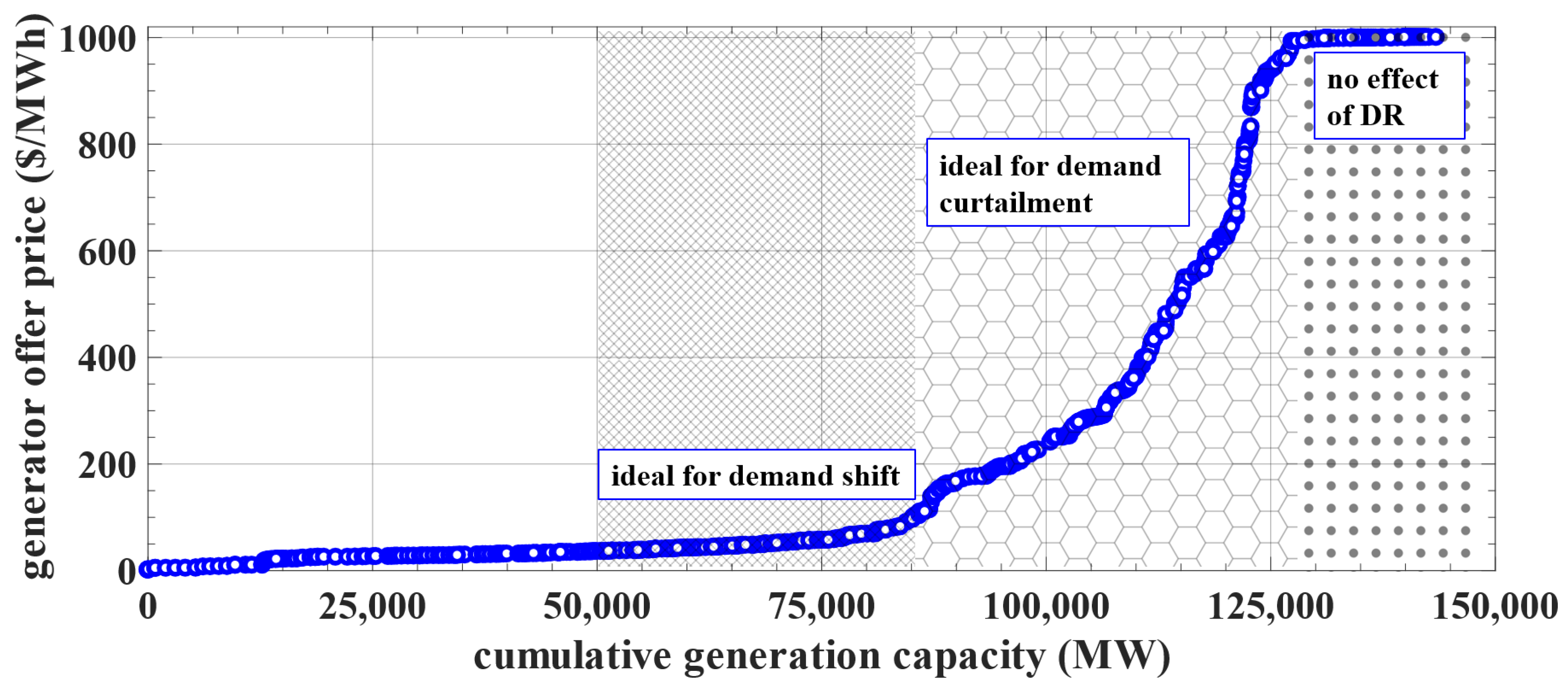
FERC Order No. 745 was a landmark order for DR that opened the energy market for DR participating as a resource. In the energy market, DR providers earn revenue based on the LMP of the bus they are operating, like other generators in the day-ahead market. Figure 1 represents the cumulative generator offer curve of the PJM day-ahead market for 27 January 2014. Each blue circle represents a generator and its offer price, the size of each generator given by the gap between each circle in the positive direction of the x-axis. Without considering any line or voltage limits, the marginal energy cost will be determined by the intersection of total demand and this supply curve. A DR offer in the day-ahead market should be offered at an intra-marginal price to be selected by the ISO. Analyzing the recent trends in annual system marginal price of PJM, which was 53.7 $/MWh, 38.4 $/MWh, and 31.8$/MWh for 2014–2016, respectively, DR participating as a resource in the energy market may not be economically sustainable.
Instead, if the DR is offered as a service for the energy market, the cost of the service can be treated independently from the LMP, and the DR would be compensated based on the benefit it provides to the market. The benefiting entity pays for the DR service, where the most common entities benefited are electric utilities, as DR causes a reduction in LMP, which reduces utility purchases from the bulk-market. From Figure 1, we can observe that, if the demand curve intersected the supply curve in the region shaded by the dotted-pattern, the marginal price will be high, but demand reduction would not cause a reduction in price; DR-as-a-service would not earn revenue when the system is operating in this region. When the demand intersects the supply in the region shaded by the honeycomb-pattern, a small change in demand can greatly impact the marginal price, which is the ideal region for DR in an energy market. If the DR operation can have a controllable rebound, then it would be ideal to shift the demand to the region shaded by the diamond-pattern, as additional demand will not significantly increase the marginal price. The specific values of offer price and demand shown in Figure 1 should not be considered as the absolute delimiter for each region, as this will change daily in the market. Rather, the demarcation of the regions is dependent on the shape of the daily supply curve.
3. DR-as-a-Service
Regulatory bodies have opened opportunities for non-generating resources, such as DR, to participate in various market operations. DR is being used in ancillary services for regulation and reserves. This section presents the idea of using DR-as-a-service (as opposed to a resource) to improve economic benefits to other bulk-market entities. This section presents a review of the benefits for (i) bulk-power entities willing to pay for DR-as-a-service for their financial benefits, and (ii) DR service providers and end-customers willing to trade DR-as-a-service. As providing DR-as-a-service is still in its nascent state, we have included some of the state-of-the-art research in this field. Like any new service, DR will have challenges to be solved for integration into bulk-power markets. In this section, we also provide a review of such challenges, as well as describe literature that addresses these challenges.
3.1. DR Service Buyers
3.1.1. Generators
FERC Order No. 745 was challenged by Electric Power Supply Association in court, as they did not want non-generating resources to be able to set the market LMP. If used as a resource in the energy market, DR does not provide benefits to generators, and in fact competes against them. Additionally, as discussed in Section 2.2, DR as a resource might not be economically sustainable for the DR providers; DR-as-a-service can be engineered to benefit both the DR providers and the generators.
Reducing GHG emissions has been an important topic of research in power systems. In many states where renewable portfolio standards (RPS) are enforced, traditional generating entities maintain the RPS via a credit-trading mechanism [37]; DR can be made available as a service to reduce GHG emissions [9,10,38] and can be used to trade carbon-credits. The DR service can be structured such that DR providers sell both DR (as a curtailment service) and carbon credits, and LSEs invest in the curtailment service to reduce their payments, while generating entities procure carbon-credits.
There has been a change in the generation profile over the past decade, as significant investments have been made in RES. An ISO that operates under a fair market policy must dispatch the available resources economically and securely. In general, demand is inelastic to changing market LMPs under fixed rate tariff and time-of-use (ToU) plans. Under lower demand conditions, the ISO sometimes needs to curtail or sell additional RES to adjacent load areas at negative revenue [39,40]. A consolidated demand side entity (e.g., DRA) that owns multiple resources, like distributed RES and energy storage systems (ESS), can optimize the available resources and modify the demand curve to better utilize RES while maximizing their profit through the bulk-power market [41]. A DR-as-a-service model proposed in [27] utilizes a DRX to offer DR to renewable generation and ESS entities, where the objective of the DRX is to maximize the social welfare of DR sellers and DR buyers, thus improving RES utilization.
3.1.2. Utilities/Retailers
Utilities/retailers (LSEs) are the main entities that benefit from DR [3,38,42]. In 2018, most U.S. retail markets used the fixed tariff model. DR-as-service will be beneficial for utilities that use flat rate pricing because the price at which the utility buys the bulk-power is variable, but is sold to the end-user at a fixed rate. DR can bring large changes in the bulk-power price, which may allow utilities to sell at a higher profit (purchase less peak generation) [38,42], invest in additional infrastructure, or reduce retail rates according to the public utility commission.
DR-as-a-service would also benefit those utilities that offer ToU pricing, which is fixed for certain periods of the day and season, as market prices are volatile and peak prices may occur at non-peak price ToU hours [14]. There are a few utilities that offer real-time pricing (RTP) to their customers (sell energy to the end-user at the same cost as the bulk-power market), but IBDR may not be impactful for such utilities, as the consumers pay the same energy price of the bulk-power market.
Significant charges for a utility are distribution and wheeling charges, especially if the entity is a retailer that does not own the physical infrastructure. Transmission charges are generally calculated based on the utility contribution to the coincidental peak of the system [38,43]. Using DR-as-a-service to reduce demand during such peak hours will ensure lower transmission charges for the utilities. These savings on transmission/wheeling charges are beneficial for utilities with any type of billing (flat, ToU, and RTP), as these are fixed charges based on the behavior of a few peak hours per year, irrespective of the energy price during that hour.
3.1.3. ISO/RTO
In a fair market, the ISO should not profit from the power transaction (independent entity). Market surplus—the additional revenue generated due to congestion—is returned to entities that own financial transmission rights (FTRs). System security is ensured through the use of ancillary services; DR is one of the cheapest services, as there is no additional ISO investment [44]. While other models of DR can be successful in reducing LMP spikes, DR-as-a-service can be used for other ancillary services to keep the system secure.
The transmission system operator (TSO) is an under-discussed entity in the power market, usually a monopoly and operated by the ISO. The ISO charges a fee for open access of transmission from every participating power market entity. To cater to the needs of the power producers and buyers, the TSO needs to invest in network expansion. These expensive investments can be temporarily deferred through DR, as extra transmission capacity is mostly needed during system peaks [7,38].
3.2. DR Service Sellers
The benefits for the DR providers under various PBDR and IBDR programs have been presented across the literature [18,22,45]. In this section, we discuss the additional benefits that DR providers can gain if DR is treated as a service.
3.2.1. Demand Response Aggregator
DRAs are for-profit entities that have a set of customers willing to modify their demand for incentives. The DRA provides incentives to their customers by generating revenue from selling DR to bulk-power entities. When DR is offered as a resource, the DRA must ensure the DR offer price submitted to the bulk-power market is competitive with other generator offers. The marginal generator offers have been reducing annually, as mentioned in Section 2.2, which makes it difficult for the DRA to operate in the energy market.
In the DR-as-a-service model, the DRA can submit offers to the market based on their demand portfolio, but the offer does not participate in the energy market clearing process. Instead, the DR is compensated based on the quality of service provided, so the DRA is capable of generating enough revenue to earn profit and pay incentives to participating customers [26,31,38]. Even though the DRA submits an offer price greater than the marginal energy price, the benefiting entity is able to pay for the service as the total benefit received is greater than the small quantity of DR required (which will be shown in detail in the simulation study). There are more potential buyers for DR when offered as a service, creating a more sustainable business model for the DRAs.
3.2.2. Electricity Consumers
Electricity customers that do not have advanced metering, or do not live in the right geographical location, cannot enroll in ToU or RTP-based billing models (PBDR) [15]. IBDR programs give DRAs direct control over a few electric loads to provide DR-as-a-service; the customer need not pay attention to the DR events. By informing the DRA their willingness towards the event and required incentive, the customer earns financial benefits from successful DR events. The customer can change their willingness and/or opt-out of individual DR events, unlike PBDR. Additionally, proactive customers can provide different willingness over the DR period, where they can increase DR activity during high DR price offers, and reduce when earnings are low [27]. RTP customers not participating in DR that reside in the same load area as the DR-as-a-service program will also receive benefits of the DR activity, resulting from reduced energy prices (although they will not receive the additional aggregator incentives).
Large consumers (industrial, large commercial) pay additional charges for capacity and distribution based on their contribution to the coincidental peak of the utility. By reducing their contribution during these coincidental peaks, they can save heavily on distribution and capacity charges. DR-as-a-service can be used to reduce this coincidental peak contribution.
3.3. Challenges Integrating DR-as-a-Service
There are challenges integrating any new model/service into existing deregulated bulk-power markets. This section presents the state-of-the-art industrial and research practices, and the unmet challenges of integrating DR-as-a-service into the bulk-power market.
3.3.1. Compensation, Incentives, and Penalties
From the discussion in Section 3.2.1, it is inferred that the DR service providers can gain sustainable revenue by providing DR-as-a-service. Most literature discusses the total revenue gained by the DR service providers, and the total benefit to the power market entity [27,28,35]. The total benefit and cost of DR-as-a-service discussed in prior work considers a single entity on the system (single utility). Free-riders are entities that enjoy the benefits of a service without paying. The authors in [26,31] show an estimate of the free-riders, and how much each entity benefits, but only one participant of each entity is considered. The problem is more complicated when there are multiple participants of each entity located at multiple nodes on the network, and compensation techniques for DR-as-a-service need to be designed based on multiple competing entities at different network locations.
Once the DRA receives market compensation, they must distribute incentives to the participating customers. Accurate evaluation of CBL is essential in determining incentives, and also impacts customer willingness. Liberal baseline estimation will result in losses to the DRA, while a conservative estimate punishes customers. Authors have used real data of both residential and non-residential loads from California to estimate CBL using regression models. In [46], the CBL was estimated using various time-series analysis, regression, and exponential moving average techniques for different customers based on their flexibility. The authors performed profit analysis based on each customer for each electricity market. A CBL estimation technique was discussed in [47], which attributes CBL changes for customers that already reduced their energy consumption using energy efficiency techniques.
The planning of DR happens day-ahead, but the transactions occur based on real-time market values. There are chances that a DRA offer is cleared, but fails to perform the DR. During such events, the ISO commits reserves, which can cause a spike in LMP. During such situations, the DRA and end-users that failed to perform may be penalized. During partial participation of DR, where few customer loads are curtailed with no market efficiency improvement, the DRA does not receive incentives as no entity has benefited. During such events, the DRA is obligated to pay the customers who performed DR, in-spite of paying penalties to the market, which incurs losses to the DRA.
3.3.2. DR Offer Structure
To develop realistic DR offers, the DRA must know the demand-elasticity of customers with respect to price. The elasticity depends on the type of load (e.g., residential appliances), climate (e.g., heating and cooling loads), and type of customer [48]. The bid offer should reflect the customers’ elasticity towards the incentive offered, which requires large surveys. One such work to determine the elasticity of residential consumers is presented in [49], but the responses are local to a particular region, and these responses may change over time. After obtaining such elasticity data, they must be translated to incentives based on the expected revenue to the DRA.
Residential customers comprise 40% of the total electric demand, and as such are a great potential for DR. To model a residential DR offer, the DRA must know the demand curve to the appliance level. Such information is sensitive, and is not widely available for the research community. The authors in [50] designed a technique to synthetically generate load profiles that can be used to develop DR offers. In real-world scenarios, there would be multiple DRAs competing to provide DR-as-a-service. In addition to incentives, the DRA must also consider competition in determining offer strategy.
3.3.3. DR Trigger
If DR is provided as a service, there must be a triggering mechanism to call for this service. DR currently participates in ancillary services, which are triggered by certain power system operational limits. If DR-as-a-service is used for economic purposes, a triggering mechanism must be provided. In [51], we used statistical pattern recognition to analyze day-ahead market LMP, load, and climate data to trigger the DR service during market inefficiencies. This classifier only triggers during high LMP-based inefficiencies, where load curtail bids can be evaluated. An investigative study needs to be performed to evaluate the factors that influence the impact of DR on the electricity market, and proper DR-as-a-service triggers need to be designed.
4. DRX in the Day-Ahead Market
In this work, to integrate DR-as-a-service we use a DRX—a non-profit entity working as a pool-based market under the ISO. As this entity is modeled as a market, it resembles the operation of the ISO. The sellers in this market are the DRAs that offer DR-as-a-service, and the buyers are those bulk-power market entities that benefit from the DR service (i.e., electric utilities in this work).
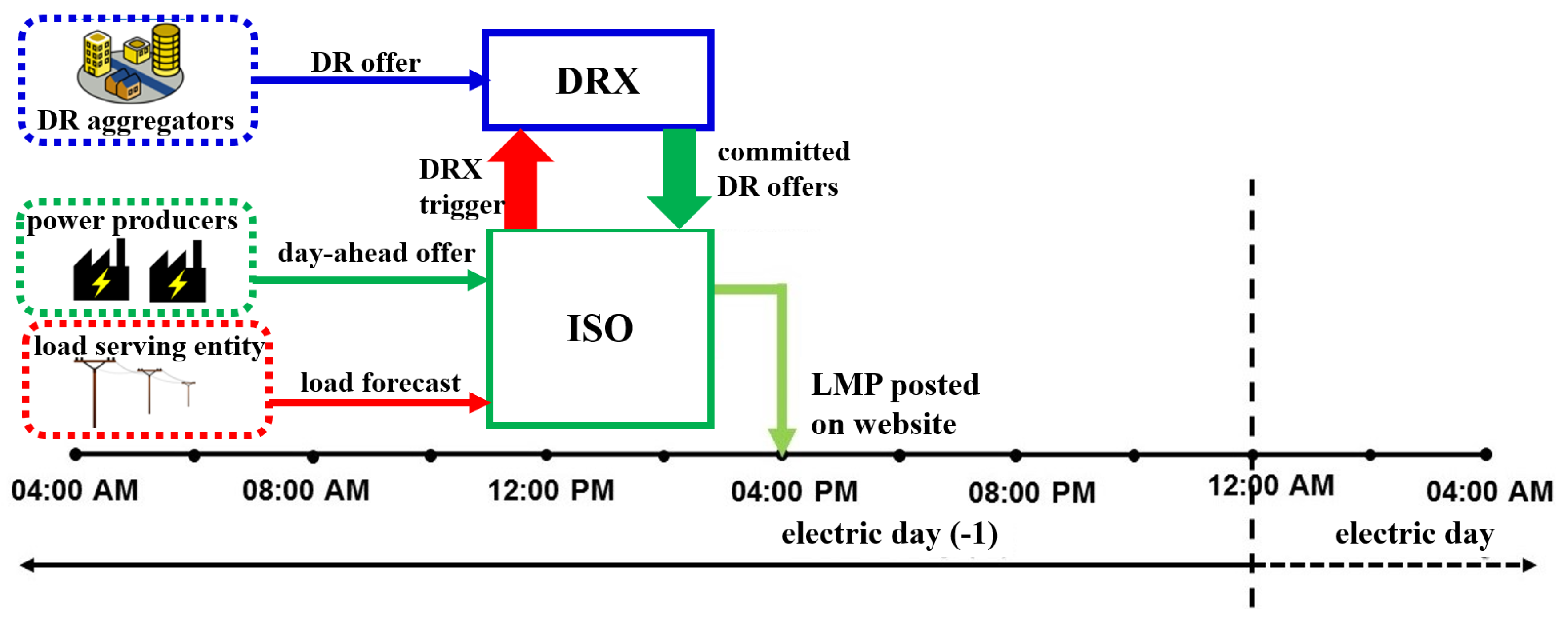
The DRX is integrated into the day-ahead energy market operation as shown in Figure 2. The day-ahead market begins its operation by accepting generator offers and utility load forecasts. The DRX operates in parallel to the ISO, and is triggered when economic inefficiency is incipient, and DR-as-a-service is required. The DRX accepts day-ahead DR offers from DRAs, and clears those DR offers that benefit the bulk-power market. The bulk-power market is settled by the ISO using DRX-cleared DR offers, and the energy market LMPs are posted in the day-ahead. The benefiting entities from DR-as-a-service compensate the DRA offers at the marginal DR cost. Part of the DRA revenue is then passed on to participating customers as incentives (i.e., IBDR).
The DRAs in this study are for-profit entities that have a set of customers that are willing to curtail and shift their scheduled loads. A DRA prepares a cumulative DR supply curve by aggregating all the DR resources within their purview. The objective of the DRX in this study is utility payment cost minimization [33]. The OPF evaluated at the DRX will have the same formulation as in Equation (1), but will now be subject to a slightly different equality constraint, as shown in Equation (6), where is the DR at load bus j at hour t, and is the LMP:
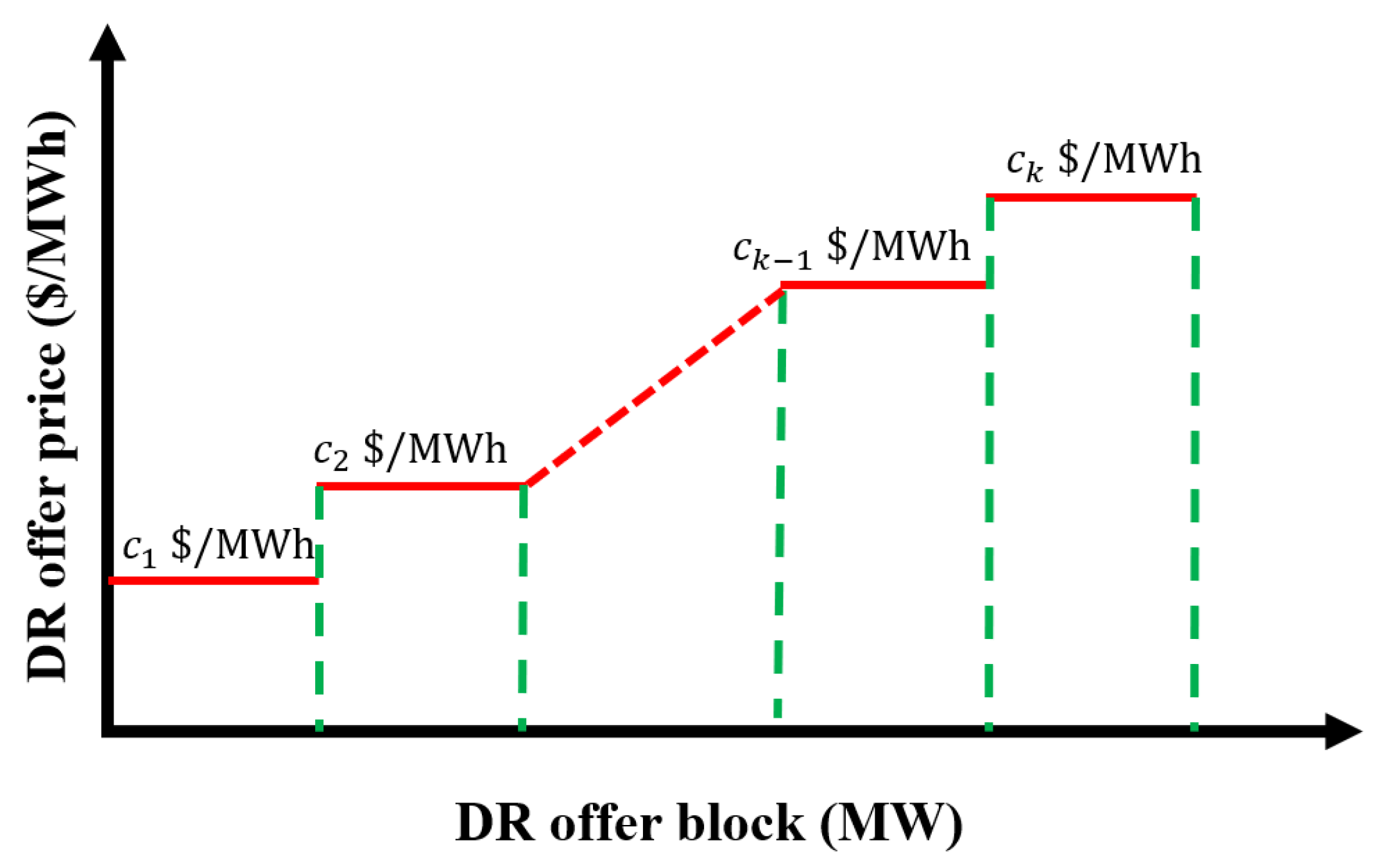
The DR offer consists of five fields: (i) bus number (location on the network where the aggregated DR is connected); (ii) the hour of DR; (iii) the offer quantity blocks and (iv) corresponding offer prices; and (v) the shift window. DR offers are constructed by the DRA based on customer curtailment elasticity. The DRA arranges the DR blocks in incremental order of price, as shown in Figure 3. The size of each block may not necessarily be equal, as a DRA may have various classes of customers with different capacities. The maximum number of blocks per DR offer is capped at an integer k, similar to generator offers in PJM being capped at 10 blocks [52].
Algorithm 1, which is used for selecting near-optimal DR offers, is based on the GENITOR version of the genetic algorithm (GA) [53]. The objective of this algorithm is to minimize the total utility payments for the ISO market, as described in Equation (7). The GA chromosome represents a solution to the optimization problem; for the DRX, the chromosome is shown in Figure 4. Each chromosome has an associated fitness value, which corresponds to the objective function of the problem (better solutions will have better fitness values). There are p chromosomes that comprise the GA population.
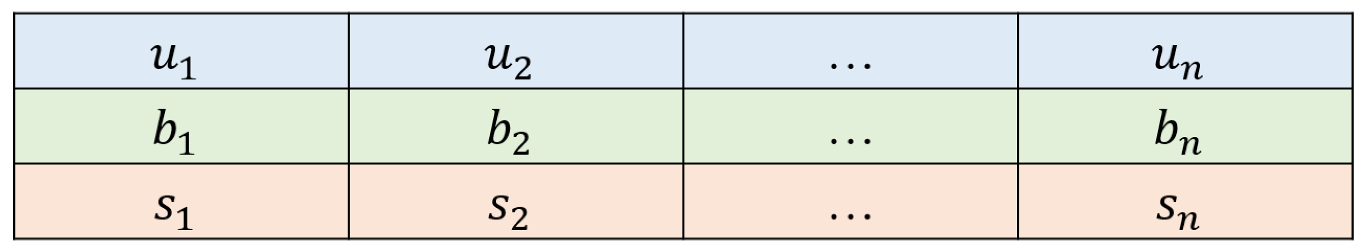
The chromosome is made up of n genes (equal to the number of DR offers submitted to the DRX for that day), where each gene in the DRX GA represents one DR offer (as described by Figure 3). Each gene is comprised of three parts: (i) the DR offer selection (shown as the top blue row); (ii) the DR block selection (middle green row); and (iii) the shift window (bottom red row). For a given gene i, if , the DR offer represented by that gene is selected by the DRX. If selected, the DR offer size and cost is provided by block , where is the number of blocks in the DR offer. The demand of the selected DR offer block is shifted to hour , where is the number of hours in the shift window, and is the number of hours to shift from the beginning of the shift window (e.g., moves the demand to the start of the shift window).
| Algorithm 1 Algorithm to select day-ahead DR offers using GA |
|
The first step of the GA is to generate an initial population that describes the DRX selection of DR offers. For each gene in the chromosome, is randomly generated as a Boolean value (with equal probability), and and are uniformly distributed in the ranges and , respectively, . The initial population is comprised of p such randomly generated chromosomes, each with n DR offers (genes). The fitness of each chromosome in the population is calculated, and put in descending order (lower fitness is better). To evaluate the fitness as mentioned in the Steps 9 and 16 of Algorithm 1, all selected offers () of a chromosome are applied to the system. Let us consider gene i with , meaning the DR offer is selected. The block number for DR offer i is obtained from , and the DR quantity and cost can be determined. These DR and shift quantities are applied to the original demand forecast of the system at hour t on load bus j. OPF is evaluated using Equation (1), subject to Equation (6), to obtain the new . Similarly, , , and are obtained . This information is used to evaluate Equations (8) and (9), where the fitness of a chromosome is the sum of these two values. If more than one DR offer is cleared at the same bus and hour, the highest offer cost of the DR offers is used as the marginal DR offer price, and all accepted DR offers are paid the same marginal price irrespective of their offer block.
After the initial population is generated, the algorithm begins its search by iterating through a selection-crossover-mutation phase (Steps 13–18 in Algorithm 1) to create two new child chromosomes (solutions). In each iteration (“generation” of the GA), two chromosomes are randomly selected using linear bias [53], shown in Equation (10), where “random()” returns a sample of a uniform random variable in the range . The function biases the choice of crossover to those chromosomes that are performing better according to a linear bias parameter, :
After selecting the two “parent” chromosomes, two points are uniformly randomly chosen between . The chromosomes swap genes within these points (two-point crossover) to create two new “child” chromosomes. Each gene in the child chromosomes has probability to mutate. If gene i mutates, the genes for and are randomly chosen using the same process as in the initial population.
The new chromosomes are evaluated for their fitness and inserted back into the population. The best p solutions are kept at every generation (elitism). The GA iterates until the maximum number of generations is reached, or there is no significant change in the fitness value in a certain fixed number of iterations. The final DR offers are selected at Step 20 for each gene with of the chromosome corresponding to the least fitness value (minimum utility payments). Both the new demand curve and the adjusted marginal energy prices are used to evaluate the LMP of each location, and are posted by the ISO as the final settlement of the market.
The GA was chosen as a proof-of-concept of the DRX clearing algorithm for its scalability in cost minimization problems [54], and has been shown to work well in many power system applications [30,55,56]. In our preliminary work, we also explored a greedy search algorithm [35]. There are multiple metaheuristic (e.g., particle swarm optimization) or classic optimization techniques for implementing cost minimization of the DRX; however, the choice of optimization is not the main contribution of this work, and does not impact the discussion of the results or the conclusions of the work.
5. Experimental Setup and Case Study
To evaluate the economic benefits of the proposed DRX market clearing technique, we prepared a simulation environment that statistically represents an actual U.S. electricity market (i.e., PJM). This section presents the simulation setup, including all algorithm parameters and inputs, and the results and discussion of a case study based on the proposed technique.
5.1. Simulation Setup
5.1.1. Power System Test Case
To illustrate the proposed multi-period DRX market clearing algorithm, a simulation was conducted on the IEEE 24-bus reliability test system (RTS) [57], chosen as it includes realistic line limits (i.e., for congestion). We chose PJM market data for this study, as most required data is available as open source [58]. The test case generator cost functions were modified to reflect the PJM market generator offer curves using the clustering method from [59]. These market-based cost functions statistically represent the supply curve of real power markets scaled to existing power system test cases. Because the supply curve represents the real power market, the LMPs generated by the augmented test case follow that of the real power market. Similarly, any load changes would yield realistic price changes that can be considered as an estimate of savings for DR services in real power markets.
Two dates were chosen for the simulation study to illustrate the DRX market clearing technique. One date had a PJM DR event (23 January 2014), and the other (27 January 2014) did not have a DR event, but had a high peak LMP [60]. We chose the non-DR event day to verify the expected advantages of using DR-as-a-service. The PJM demand curves for the specified dates were scaled to the test case using the same technique followed in [59]. MATPOWER OPF was used for running the market simulations [61] to produce LMPs at every bus. The OPF was evaluated at the same frequency as the day-ahead and real-time electricity markets (i.e., one hour resolution).
5.1.2. DRX Offer Data
To set up the DR offers for the two days mentioned above, the size of DR with respect to the demand for that day was determined to represent the actual DR capacity of the PJM market. On 23 January 2014, as per the annual report of PJM [60], the total committed DR for the DR event was 4405 MW at hour 2:00 p.m. Thirteen of the twenty load zones of PJM participated in this DR event, which had a total demand forecast of 71,946 MW for the same hour. Thus, the percent of demand committed for DR was of the total demand forecast.
Even though the proposed market clearing technique is capable of selecting multiple DR offers from a single bus, in this case study, at most a single offer for each bus at a given time was generated. The maximum curtailment per offer was restricted to 4–7% of the demand on that bus (similar to the PJM case), and only eight (half of the load buses) were allowed to have DR offers. Even though the number of blocks per DR offer can vary, for this simulation, the number of blocks per offer was fixed at . The five offer blocks were considered to be equally sized (i.e., each offer block was of 4–7% of , where is the demand of the bus j at time t for the test case with PJM scaled demand).
The literature is scarce for designing optimal incentive prices for consumers. Determining the optimal incentive is a sociology research topic, which is not in the scope of this paper. To determine the price of the DR offer supply curves, we developed the DR offers based on the range of retail electricity prices of the PJM region, with the offer prices for each block randomly selected in the range of 50–300 $/MWh (in ascending order).
The peak hours of PJM (8:00 a.m. to 11:00 p.m.) were chosen to be the DR curtailment hours. To mitigate rebound for this simulation, DR was allowed to be shifted to any other time during the day. This DR shift flexibility was chosen for this case study to analyze the capability of the algorithm to shift demand to a time that does not significantly increase utility payments (i.e., LMP). Because the demand is capable of being shifted to any hour of the day (except the curtailment hour), the shift window size for every offer is set to between 1:00 a.m. to 12:00 a.m. With the above conditions, DR offers were generated for each day. These numbers are chosen for this system, but the DRX clearing method described above works for DR offers generated from any source (e.g., real customer data, state-of-the-art literature DR techniques).
5.1.3. GA Parameters
The GA for the case study used a population size . Each chromosome contained genes (i.e., the number of DR offers). At each generation, the index for the parent chromosomes are chosen using the linear bias function in Equation (10) using a bias parameter , which means that the best solution according to its fitness has a 50% greater chance of being selected than the median solution. For each child chromosome, each gene has a probability of mutation . The GA continues until stopping criteria of 10,000 generations is reached, or 300 consecutive generations without improvement in the best fitness value.
5.2. Simulation Results and Discussion
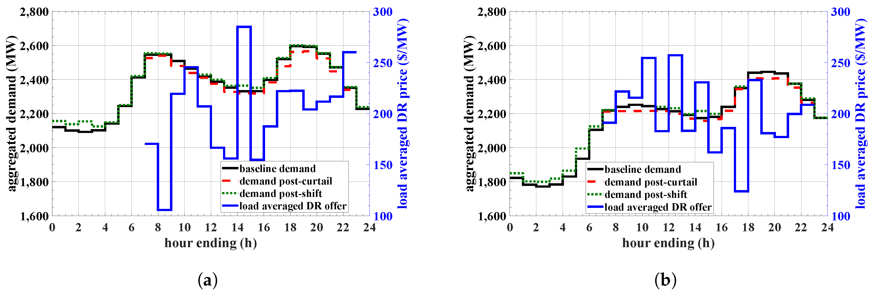
To determine the impact of a DRX minimizing utility payments in a day-ahead market, we analyzed the weighted-load average system marginal energy price, and the utility payments before and after DR. Although our proposed DRX model was described with a trigger in Section 3, we have not incorporated any technique for triggering the DRX in this paper as we have pre-selected two dates that were candidates for DR-as-a-service. The simulations were conducted in MATLAB R2017a on an Intel Core i7 3.6 GHz computer with 16 GB of RAM. The GA took 42:06 and 53:11 min to converge for 23 January and 27 January, respectively. Out of 128 offers, 66 were selected and scheduled for 23 January, and 71 were selected for 27 January. A detailed discussion of the impact of these DR offers on the bulk-power market are presented in this section. As discussed in Section 5.1.1, the hourly demand on the augmented test case was derived by scaling down the PJM system hourly demand. This demand serves as the baseline demand for the two days, and is represented by the solid black line in Figure 5. The solid blue line with the right y-axis represents the marginal DR cost for each DR hour. Based on the DR offers selected by DRX for the two days, the demand curve is modified for demand curtailment as shown by the red dashed curve, and the demand rebound (shift) is represented by the green dotted curve. The DR offers considered in this study (described in Section 5.1.2) operate only between 8:00 a.m. to 11:00 p.m., which is reflected in Figure 5 where the red dashed line only varies between those hours. All demand plots in Figure 5 are the aggregated demand of the load buses on the test case. Because the shift hours considered in those offers were flexible throughout the day, the demand rebound is spread across the day and mostly concentrated during off-peak hours.
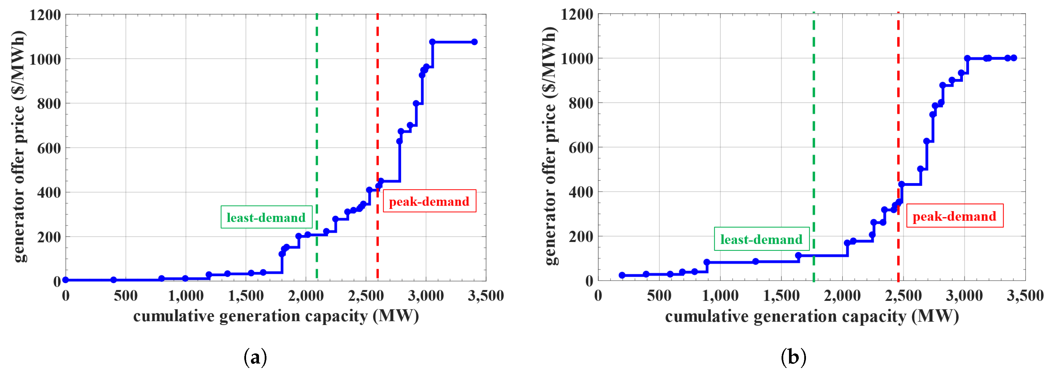
For a given time period, DR is offered on multiple load buses. Based on the cleared offers, curtailment and rebound can occur at the same hour, but at different load buses. This can be observed in Figure 5, where in most hours curtailment and shift happen simultaneously. The magnitude of curtailment is relatively high during the peak-hours (6:00 p.m.–9:00 p.m.), and shift is relatively high during the mid-day demand valley (1:00 p.m.–3:00 p.m.). The objective of the DRX is to minimize utility payments, which occurs when curtailment offers are selected during those hours when the demand intersects the supply curve at a steep slope, and shifts the demand to those hours when the demand intersects the flat supply curve (as shown in Figure 1). In this case study, the peak DR activity occurred on 23 January at hour 6:00 p.m. During this DR period, 42.8 MW was curtailed out of the aggregated system demand of 2520.5 MW, i.e., 1.7% curtailment. For the 27 January simulation, the peak curtailment of 1.6% was deployed during hour 8:00 p.m. The number of generators in a test case is much lower than in the real network. The IEEE 24-bus RTS consists of 32 generators, with modified cost functions as described in the Section 5.1.1. Cumulative generator supply curves similar to Figure 1 were developed for the augmented test case for the two simulation dates, as shown in Figure 6. Even though the test case has significantly fewer generators than the real system, the supply curve in this simulation is statistically similar to the real PJM system curve of the same day in terms of price band and shape. The blue-dots represent each generator on the test case with the corresponding peak offer price. The daily system load is between the dashed-green and dashed-red lines, representing the daily minimum and peak demand, respectively. A steeper peak and flatter base supply curve represents ideal conditions for DR, as small changes in demand can result in significant decrease of LMP and utility payments. The supply curve of 27 January, shown in Figure 6b, is steeper when compared to 23 January, shown in Figure 6a, in the range of demand for the respective days. Thus, between the two days, 27 January is expected to perform better for DR.
For brevity, we only analyze 27 January in detail in Figure 5b, where we can observe the loads are always curtailed when the CBL is above 2200 MW. By observing the corresponding supply curve in Figure 6b, it can be confirmed that the curve is steeper starting at 2250 MW. The supply curve has a flat offer price between the minimum demand (1770 MW) and 2050 MW, and, as a result, we can observe most of the loads are shifted to hours when the demand falls below 2000 MW. These observations show that DR-as-a-service is ideal for curtailing when the supply curve is steep, and shifting to time periods when the supply curve is relatively flat.
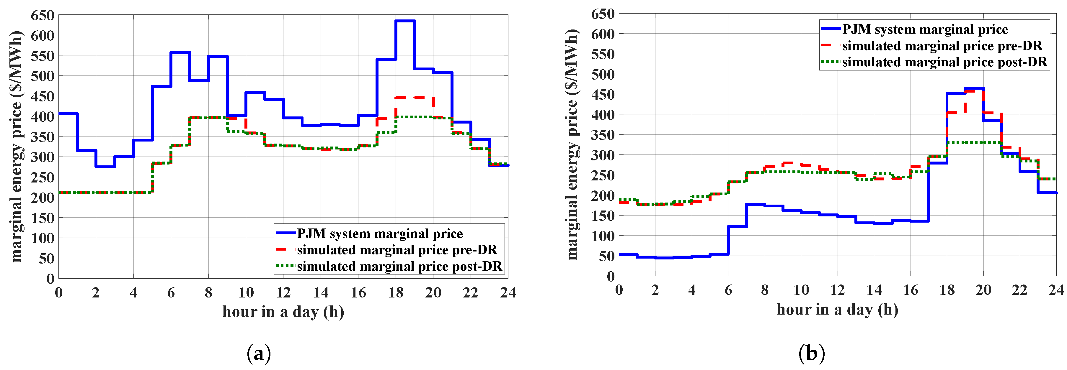
In Figure 7, the solid blue curve is the PJM system marginal price, and the red dashed line is the simulated marginal price based on the scaled demand of PJM. An exact reproduction of PJM prices is not possible, as the test case network structure and number of generation units is significantly different than the real system. As discussed in Section 5.1.1, we used the augmented test case of the IEEE 24-bus system to represent the PJM network marginal prices. With the available data resources, the augmented test case better emulates the real PJM marginal prices than the default fuel-based cost curves (shown in detail in [59]), observed for the marginal prices in Figure 7b during the evening peak hours that match that of the real system.
In the test case, the marginal price at the peak demand (∼450 $/MWh at 2600 MW) from the supply curve in Figure 6a matches the maximum marginal price (∼450 $/MWh at 7:00 p.m.) in the pre-DR case in Figure 7a for 23 January. However, in the 27 January case, the pre-DR marginal price at the peak hour was ∼450 $/MWh at 8:00 p.m. in Figure 7b, where the marginal offer at this peak demand was lower at ∼350 $/MWh for 2450 MW. This is evidence of network congestion, indicating the cheaper generator (∼350 $/MWh) could not be dispatched due to network constraints, and instead the next available generator offer of ∼450 $/MWh was cleared. This also explains the large decrease in LMP post-DR between hours 6:00 p.m. and 9:00 p.m. for 27 January.
Even though the entire curtailed demand (328 MW on 23 January and 340 MW on 27 January) was shifted to another hour, there is no significant increase in the marginal price during any off-peak hour. This holds true because the algorithm was designed to select only those DR offers that will reduce utility payments during curtailment, while simultaneously not significantly increasing the payments during rebound hours. Because the DRX allows DR offers as a service rather than resource, we can observe the system marginal price is only set by the generators that are part of the supply curve. The DR marginal price, shown in Figure 7, only serves as the price for the DR service, but does not set the marginal price of energy in the bulk-power market.
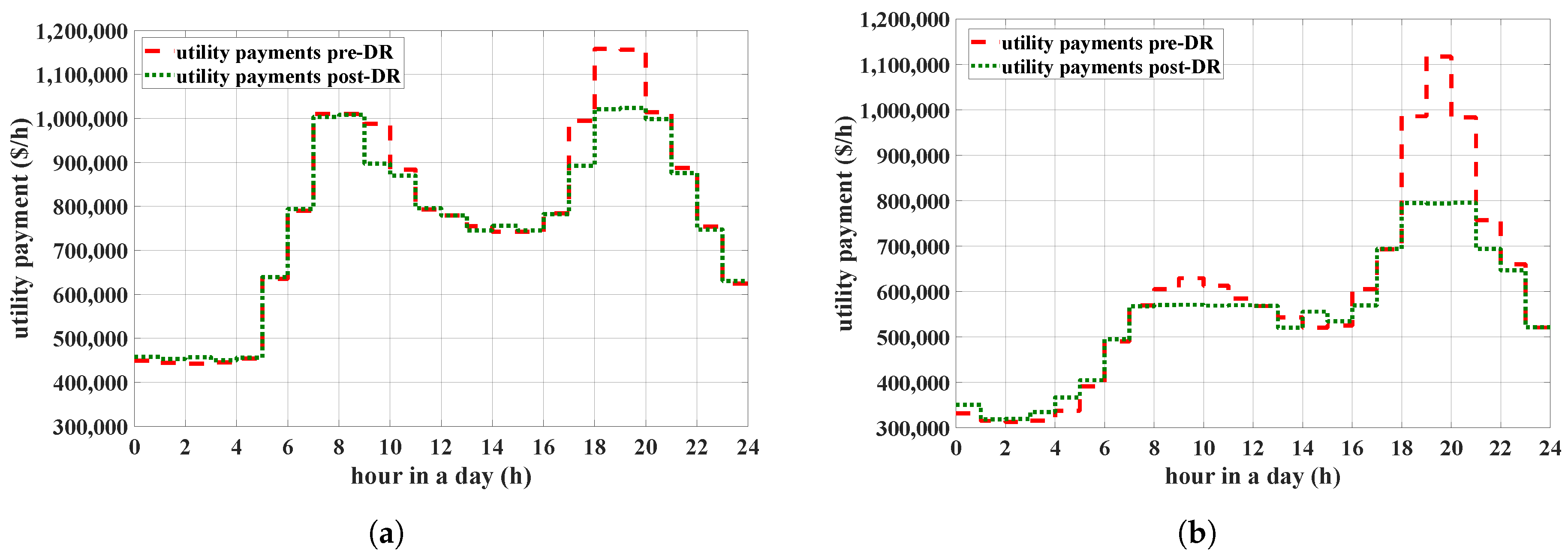
The objective function of the DRX in this study was to minimize utility payments, which depends on the aggregated demand and LMP of the load bus. From the discussion above, it was found that the LMP is reduced during peak-hours, and does not significantly increase during off-peak hours. This directly reflects utility payment reductions, shown in Figure 8. The red dashed lines represent the hourly payments before DR, and the green dotted line represents the payments after DR. It can be observed in Figure 8b that between hours 6:00 p.m. and 9:00 p.m., the utility payments reduced to the same point. This is likely because pre-DR, the marginal generator was creating an LMP for a small quantity of demand (e.g., the ∼450 $/MWh generator discussed above). Just like in the marginal energy plot, we can confirm there is no significant increase in utility payments after the DR and demand shift.
Table 1 presents a comparison of the utility payments and generator revenue before and after DR for both days. The surplus described in this table is the market surplus, which is the difference between the utility payments and generator revenue. Market surplus is an indication of congestion in the network. DR-as-a-service resulted in higher benefits in terms of utility payment reduction on 27 January than 23 January because of the difference in generator supply curves of these two days (discussed earlier in this section). The peak demand on 27 January intersects on a much steeper region of the supply curve, where the small changes in demand resulted in larger reduction of LMP when compared to the supply curve of 23 January. The largest factor in utility payment reduction is the decrease in LMP, which is highly dependent on the generator supply curve and network congestion. The utility saved 6.2% in payments by spending only 0.5% of the initial payment for 27 January, and 2.1% savings by spending 0.4% of the initial payment for 23 January. The results for 23 January show savings in utility payments, but the market surplus of the system has increased when compared to the pre-DR case.
6. Conclusions
An extended review of DR in electricity markets in terms of advantages, challenges, and opportunities was presented. In this work, we designed a market model, the DRX, to integrate DR-as-a-service into existing energy markets. The DRX model minimizes utility payments using DR services, while simultaneously providing an opportunity for DR service providers to offer the incremental cost of the service. A multi-period market clearing algorithm to select DR offers was proposed, where DR offers have both curtailment and shift information. The multi-period nature of the algorithm ensures that the selected DR offers do not adversely affect utility payments when the demand rebounds post-DR. The algorithm was implemented using a GA on an augmented IEEE 24-bus RTS test case that statistically represents the PJM day-ahead energy market. The results of the case study of the proposed DRX market clearing method determined important factors that influence the ability of DRX to reduce utility payments.
From the two simulations on the augmented IEEE RTS-79 test case, significant reduction in utility payments was obtained for both days. The utility payments reduced by 6.2% for 27 January, creating a benefit of $864,199 by spending $69,955 on the DR service, and $393,066 of savings by spending a similar amount ($68,092) for the DR service for 27 January. The peak DR deployment for 23 and 27 January was 1.7% and 1.6% of the aggregated demand of the system, respectively. By comparing the results of the two days, it is clear that the benefit (utility payments) from DR-as-a-service depends heavily on the generator supply curve, demand, and the state of congestion in the network. It is important that the demand during the load curtailment meets the supply curve at a steep slope region, where small changes in demand can result in significant savings for utilities and customers. This factor is why 27 January shows greater savings when compared to 23 January, even though the quantity of DR curtailed is similar. Additionally, the demand rebound (shift) should be planned such that it is scheduled during hours where the supply curve has a relatively flat slope so the price during that time does not significantly increase.
Even though the quantity of DR was chosen statistically to represent the real installed DR capacity of a market, there is still a need to design methods to determine DR offer blocks based on real customer load models, and offer prices based on customer willingness models. Along with the realistic DR offer blocks and costs, the shift window should be developed with realistic window sizes according to customer behavior.
Author Contributions
V.D. conducted the formal analysis, while T.M.H. was responsible for conceptualizing, supervising, editing, and funding the work.
Funding
This work is supported by the SDSU Electrical Engineering Ph.D. fund and by the National Science Foundation under Grant No. ECCS-1608722.
Conflicts of Interest
The authors declare no conflict of interest.
References
- U.S. Federal Energy Regulatory Commission. Order No. 888, Promoting Wholesale Competition through Open Access Non-Discriminatory Transmission Services by Public Utilities; FERC: Washington, DC, USA, 1996. Available online: http://www.ferc.gov/legal/maj-ord-reg/land-docs/rm95-8-00v.txt (accessed on 10 October 2018).
- U.S. Department of Energy. Benefits of Demand Response in Electricity Markets and Recommendations for Achieving Them; A Report to the United States Congress Pursuant to Section 1252 of the Energy Policy Act of 2005; U.S. DoE: Washington, DC, USA, 2006. Available online: http://eetd.lbl.gov/ea/EMP/reports/congress-1252d.pdf (accessed on 10 October 2018).
- Albadi, M.; El-Saadany, E. A Summary of Demand Response in Electricity Markets. Electr. Power Syst. Res. 2008, 78, 1989–1996. [Google Scholar] [CrossRef]
- Aghaei, J.; Alizadeh, M.I. Demand response in smart electricity grids equipped with renewable energy sources: A review. Renew. Sustain. Energy Rev. 2013, 18, 64–72. [Google Scholar] [CrossRef]
- Siano, P. Demand response and smart grids—A survey. Renew. Sustain. Energy Rev. 2014, 30, 461–478. [Google Scholar] [CrossRef]
- Wang, F.; Xu, H.; Xu, T.; Li, K.; Shafie-khah, M.; Catalão, J.P. The values of market-based demand response on improving power system reliability under extreme circumstances. Appl. Energy 2017, 193, 220–231. [Google Scholar] [CrossRef]
- Dehnavi, E.; Abdi, H. Determining Optimal Buses for Implementing Demand Response as an Effective Congestion Management Method. IEEE Trans. Power Syst. 2017, 32, 1537–1544. [Google Scholar] [CrossRef]
- Reddy, S.S. Multi-Objective Based Congestion Management Using Generation Rescheduling and Load Shedding. IEEE Trans. Power Syst. 2017, 32, 852–863. [Google Scholar]
- Stern, F.; Shober, M.; Tanner, M.; Violette, D. Greenhouse Gas Reductions from Demand Response: Impacts in Three U.S. Markets. In Proceedings of the 2016 International Energy Policies and Programmes Evaluation Conference, Amsterdam, The Netherlands, 7–9 June 2016. [Google Scholar]
- Sharma, S.; Durvasulu, V.; Celik, B.; Suryanarayanan, S.; Hansen, T.M.; Maciejewski, A.A.; Siegel, H.J. Metrics- Based Assessment of Sustainability in Demand Response. In Proceedings of the IEEE 15th International Conference on Smart City, Bangkok, Thailand, 18–20 December 2017. [Google Scholar]
- Cappers, P.; Goldman, C.; Kathan, D. Demand response in U.S. electricity markets: Empirical evidence. Energy 2010, 35, 1526–1535. [Google Scholar] [CrossRef] [Green Version]
- Federal Energy Regulatory Commission Staff Team. Assessment of Demand Response and Advanced Metering; FERC: Washington, DC, USA, 2017. Available online: https://www.ferc.gov/legal/staff-reports/2017/DR-AM-Report2017.pdf (accessed on 10 October 2018).
- Ponnaganti, P.; Pillai, J.R.; Bak-Jensen, B. Opportunities and challenges of demand response in active distribution networks. Wiley Interdiscip. Rev. Energy Environ. 2018, 7, 16. [Google Scholar] [CrossRef]
- Zhong, H.; Xie, L.; Xia, Q. Coupon Incentive-Based Demand Response: Theory and Case Study. IEEE Trans. Power Syst. 2013, 28, 1266–1276. [Google Scholar] [CrossRef]
- Cappers, P.; Hans, L.; Scheer, R. American Recovery and Reinvestment Act of 2009: Interim Report on Customer Acceptance, Retention, and Response to Time-Based Rates from the Consumer Behavior Studies; Energy Analysis and Environmental Impacts Division Lawrence Berkeley National Laboratory: Berkely, CA, USA, 2015. Available online: https://emp.lbl.gov/sites/all/files/lbnl1830290.pdf (accessed on 10 October 2018).
- Haider, H.T.; See, O.H.; Elmenreich, W. A review of residential demand response of smart grid. Renew. Sustain. Energy Rev. 2016, 59, 166–178. [Google Scholar] [CrossRef]
- Palensky, P.; Dietrich, D. Demand Side Management: Demand Response, Intelligent Energy Systems, and Smart Loads. IEEE Trans. Ind. Inform. 2011, 7, 381–388. [Google Scholar] [CrossRef] [Green Version]
- Chen, Z.; Wu, L.; Fu, Y. Real-Time Price-Based Demand Response Management for Residential Appliances via Stochastic Optimization and Robust Optimization. IEEE Trans. Smart Grid 2012, 3, 1822–1831. [Google Scholar] [CrossRef]
- U.S. Federal Energy Regulatory Commission. Order No. 719, Wholesale Competition in Regions with Organized Electric Markets; FERC: Washington, DC, USA, 2008. Available online: https://www.ferc.gov/whats-new/comm-meet/2008/101608/E-1.pdf (accessed on 10 October 2018).
- Hu, Q.; Li, F.; Fang, X.; Bai, L. A Framework of Residential Demand Aggregation with Financial Incentives. IEEE Trans. Smart Grid 2018, 9, 497–505. [Google Scholar] [CrossRef]
- Kang, J.; Lee, J.H. Data-Driven Optimization of Incentive-based Demand Response System with Uncertain Responses of Customers. Energies 2017, 10, 17. [Google Scholar] [CrossRef]
- Asadinejad, A.; Tomsovic, K. Optimal use of incentive and price based demand response to reduce costs and price volatility. Electr. Power Syst. Res. 2017, 144, 215–223. [Google Scholar] [CrossRef]
- U.S. Federal Energy Regulatory Commission. Order No. 745, Demand Response Compensation in Organized Wholesale Energy Markets; FERC: Washington, DC, USA, 2011. Available online: https://www.ferc.gov/EventCalendar/Files/20110315105757-RM10-17-000.pdf (accessed on 10 October 2018).
- Su, C.; Kirschen, D. Quantifying the Effect of Demand Response on Electricity Markets. IEEE Trans. Power Syst. 2009, 24, 1199–1207. [Google Scholar]
- Khodaei, A.; Shahidehpour, M.; Bahramirad, S. SCUC with Hourly Demand Response Considering Intertemporal Load Characteristics. IEEE Trans. Smart Grid 2011, 2, 564–571. [Google Scholar] [CrossRef]
- Nguyen, D.T.; Negnevitsky, M.; de Groot, M. Pool-Based Demand Response Exchange—Concept and Modeling. IEEE Trans. Power Syst. 2011, 26, 1677–1685. [Google Scholar] [CrossRef]
- Wu, H.; Shahidehpour, M.; Alabdulwahab, A.; Abusorrah, A. Demand Response Exchange in the Stochastic Day-Ahead Scheduling with Variable Renewable Generation. IEEE Trans. Sustain. Energy 2015, 6, 516–525. [Google Scholar] [CrossRef]
- Shafie-khah, M.; Heydarian-Forushani, E.; Golshan, M.E.H.; Moghaddam, M.P.; Sheikh-El-Eslami, M.K.; Catalão, J.P.S. Strategic Offering for a Price-Maker Wind Power Producer in Oligopoly Markets Considering Demand Response Exchange. IEEE Trans. Ind. Inform. 2015, 11, 1542–1553. [Google Scholar] [CrossRef]
- Nguyen, H.T.; Le, L.B.; Wang, Z. A Bidding Strategy for Virtual Power Plants with the Intraday Demand Response Exchange Market Using the Stochastic Programming. IEEE Trans. Ind. Appl. 2018, 54, 3044–3055. [Google Scholar] [CrossRef]
- Hansen, T.M.; Roche, R.; Suryanarayanan, S.; Maciejewski, A.A.; Siegel, H.J. Heuristic Optimization for an Aggregator-Based Resource Allocation in the Smart Grid. IEEE Trans. Smart Grid 2015, 6, 1785–1794. [Google Scholar] [CrossRef]
- Nguyen, D.T.; Negnevitsky, M.; de Groot, M. Walrasian Market Clearing for Demand Response Exchange. IEEE Trans. Power Syst. 2012, 27, 535–544. [Google Scholar] [CrossRef]
- Reddy, S.; Panwar, L.K.; Panigrahi, B.K.; Kumar, R. Computational Intelligence for Demand Response Exchange Considering Temporal Characteristics of Load Profile via Adaptive Fuzzy Inference System. IEEE Trans. Emerg. Top. Comput. Intell. 2018, 2, 235–245. [Google Scholar]
- Luh, P.B.; Blankson, W.E.; Chen, Y.; Yan, J.H.; Stern, G.A.; Chang, S.C.; Zhao, F. Payment cost minimization auction for deregulated electricity markets using surrogate optimization. IEEE Trans. Power Syst. 2006, 21, 568–578. [Google Scholar] [CrossRef]
- Durvasulu, V.; Syahril, H.; Hansen, T.M. A Framework for Integrating Demand Response into Bulk Power Markets. In Proceedings of the 7th International Conference & Workshop REMOO 2017, Venice, Italy, 10–12 May 2017. [Google Scholar]
- Durvasulu, V.; Syahril, H.; Hansen, T.M. A genetic algorithm approach for clearing aggregator offers in a demand response exchange. In Proceedings of the 2017 IEEE Power Energy Society General Meeting, Chicago, IL, USA, 16–20 July 2017. [Google Scholar]
- The Market Monitoring Unit, PJM. State of the Market Report for PJM 2016. Technical Report. Monitoring Analytics LLC, 2017. Available online: http://www.monitoringanalytics.com/reports/PJM_State_of_the_Market/2016/2016-som-pjm-volume2.pdf (accessed on 10 October 2018).
- Yin, H.; Powers, N. Do state renewable portfolio standards promote in-state renewable generation? Energy Policy 2010, 38, 1140–1149. [Google Scholar] [CrossRef]
- O’Connell, N.; Pinson, P.; Madsen, H.; O’Malley, M. Benefits and challenges of electrical demand response: A critical review. Renew. Sustain. Energy Rev. 2014, 39, 686–699. [Google Scholar] [CrossRef]
- California ISO. What the Duck Curve Tells Us about Managing a Green Grid. Available online: https://www.caiso.com/Documents/FlexibleResourcesHelpRenewables_FastFacts.pdf (accessed on 10 October 2018).
- Zhao, Z.; Wu, L. Impacts of High Penetration Wind Generation and Demand Response on LMPs in Day- Ahead Market. IEEE Trans. Smart Grid 2014, 5, 220–229. [Google Scholar] [CrossRef]
- Rahimi, F.; Ipakchi, A. Demand Response as a Market Resource Under the Smart Grid Paradigm. IEEE Trans. Smart Grid 2010, 1, 82–88. [Google Scholar] [CrossRef]
- Wu, L. Impact of price-based demand response on market clearing and locational marginal prices. IET Gener. Transm. Distrib. 2013, 7, 1087–1095. [Google Scholar] [CrossRef]
- Liu, Z.; Wierman, A.; Chen, Y.; Razon, B.; Chen, N. Data center demand response: Avoiding the coincident peak via workload shifting and local generation. Perform. Eval. 2013, 70, 770–791. [Google Scholar] [CrossRef] [Green Version]
- Ma, O.; Alkadi, N.; Cappers, P.; Denholm, P.; Dudley, J.; Goli, S.; Hummon, M.; Kiliccote, S.; MacDonald, J.S.; Matson, N. Demand Response for Ancillary Services. IEEE Trans. Smart Grid 2013, 4, 1988–1995. [Google Scholar] [CrossRef]
- Safdarian, A.; Fotuhi-Firuzabad, M.; Lehtonen, M. Integration of Price-Based Demand Response in DisCos’ Short-Term Decision Model. IEEE Trans. Smart Grid 2014, 5, 2235–2245. [Google Scholar] [CrossRef]
- Wijaya, T.K.; Vasirani, M.; Aberer, K. When Bias Matters: An Economic Assessment of Demand Response Baselines for Residential Customers. IEEE Trans. Smart Grid 2014, 5, 1755–1763. [Google Scholar] [CrossRef] [Green Version]
- Lee, J.; Yoo, S.; Kim, J.; Song, D.; Jeong, H. Improvements to the customer baseline load (CBL) using standard energy consumption considering energy efficiency and demand response. Energy 2018, 144, 1052–1063. [Google Scholar] [CrossRef]
- Sarker, M.R.; Ortega-Vazquez, M.A.; Kirschen, D.S. Optimal Coordination and Scheduling of Demand Response via Monetary Incentives. IEEE Trans. Smart Grid 2015, 6, 1341–1352. [Google Scholar] [CrossRef]
- Asadinejad, A.; Rahimpour, A.; Tomsovic, K.; Qi, H.; Chen, C.F. Evaluation of residential customer elasticity for incentive based demand response programs. Electr. Power Syst. Res. 2018, 158, 26–36. [Google Scholar] [CrossRef]
- Hansen, T.M.; Chong, E.K.P.; Suryanarayanan, S.; Maciejewski, A.A.; Siegel, H.J. A Partially Observable Markov Decision Process Approach to Residential Home Energy Management. IEEE Trans. Smart Grid 2018, 9, 1271–1281. [Google Scholar] [CrossRef]
- Durvasulu, V.; Hansen, T.M. Classifying day-ahead electricity markets using pattern recognition for demand response. In Proceedings of the North American Power Symposium (NAPS), Denver, CO, USA, 18–20 September 2016. [Google Scholar]
- PJM, Cost Development Subcommittee. PJM Manual 15: Cost Development Guidelines. Available online: http://www.pjm.com/~/media/documents/manuals/m15.ashx (accessed on 10 October 2018).
- Whitley, L.D. The GENITOR Algorithm and Selection Pressure: Why Rank-Based Allocation of Reproductive Trials is Best. In Proceedings of the Third International Conference on Genetic Algorithms, Fairfax, VA, USA, 4–7 June 1989; Volume 89, pp. 116–123. [Google Scholar]
- Vardakas, J.S.; Zorba, N.; Verikoukis, C.V. A Survey on Demand Response Programs in Smart Grids: Pricing Methods and Optimization Algorithms. IEEE Commun. Surv. Tutor. 2015, 17, 152–178. [Google Scholar] [CrossRef]
- Zhao, Z.; Lee, W.C.; Shin, Y.; Song, K. An Optimal Power Scheduling Method for Demand Response in Home Energy Management System. IEEE Trans. Smart Grid 2013, 4, 1391–1400. [Google Scholar] [CrossRef]
- Neves, D.; Silva, C.A. Optimal electricity dispatch on isolated mini-grids using a demand response strategy for thermal storage backup with genetic algorithms. Energy 2015, 82, 436–445. [Google Scholar] [CrossRef]
- IEEE RTS Task Force of APM Subcommittee. IEEE Reliability Test System. IEEE PAS 1979, 98, 2047–2054. [Google Scholar]
- PJM Interconnection. Daily Energy Market Offer Data. Available online: http://www.pjm.com/markets-and-operations/energy/real-time/historical-bid-data/unit-bid.aspx (accessed on 10 October 2018).
- Durvasulu, V.; Hansen, T.M. Market-Based Generator Cost Functions for Power System Test Cases. IET Res. J. 2015, 1–12. [Google Scholar] [CrossRef]
- The Market Monitoring Unit, PJM. State of the Market Report for PJM 2014. Technical Report. Monitoring Analytics LLC, 2015. Available online: http://www.monitoringanalytics.com/reports/PJM_State_of_the_Market/2014/2014-som-pjm-volume2.pdf (accessed on 10 October 2018).
- Zimmerman, R.D.; Murillo-Sánchez, C.E.; Thomas, R.J. MATPOWER: Steady-state operations, planning, and analysis tools for power systems research and education. IEEE Trans. Power Syst. 2011, 26, 12–19. [Google Scholar] [CrossRef]
Figure 1.
Cumulative generator supply curve of all participating in PJM day-ahead market for 27 January 2014. Each generator is represented as a blue dot, and the shaded patterns represent regions favorable for shift (grid), curtail (honeycomb), and no activity (dots) from left to right, respectively.

Figure 2.
Day-ahead bulk-power market operation time-line with an integrated DRX.

Figure 3.
Representation of a DR offer block structure with k offer segments, where each block is comprised of an amount (MW) and offer price ($/MWh).
Figure 3.
Representation of a DR offer block structure with k offer segments, where each block is comprised of an amount (MW) and offer price ($/MWh).

Figure 4.
The structure of the GA chromosome with n DR bids. Each gene (representing one DR offer) is comprised of (i) the DR offer selection (top blue row), where indicates the offer is selected, (ii) the DR block selection (middle green row), where, if selected, the DR offer would use bid block , and (iii) the shift hour (bottom red row), where, if selected, the DRA would shift the demand to this hour.

Figure 5.
The cumulative baseline load for each hour across the network (solid black line), compared to the demand post-curtailment (red dotted line) and demand post-shift (green dotted line) for the day of (a) 23 January 2014, and (b) 27 January 2014. The solid blue line represents the weighted-load average DR cost for each hour of DR.

Figure 6.
Generator supply curve for the test case (solid blue line), with each generator represented by a dot for the day of (a) 23 January 2014 and (b) 27 January 2014. The dashed green line represents the minimum daily demand, and the dashed red line represents the peak daily demand for each respective day.

Figure 7.
Actual marginal energy price for the PJM interconnection (solid blue line) compared to the pre-DR marginal price (dashed red line) and the post-DR price (dotted green line) for (a) 23 January 2014, and (b) 27 January 2014.
Figure 7.
Actual marginal energy price for the PJM interconnection (solid blue line) compared to the pre-DR marginal price (dashed red line) and the post-DR price (dotted green line) for (a) 23 January 2014, and (b) 27 January 2014.

Figure 8.
Comparison of utility payments pre-DR (red dashed line), and post-DR (green dotted line) for (a) 23 January 2014, and (b) 27 January 2014.
Figure 8.
Comparison of utility payments pre-DR (red dashed line), and post-DR (green dotted line) for (a) 23 January 2014, and (b) 27 January 2014.


Table 1.
Comparison of payments and revenue for pre-DR and post-DR conditions (in $).
| Date | Case | Utility Payments | Generator Revenue | Surplus | DR Operation Cost | Payment Benefit |
|---|---|---|---|---|---|---|
| 23 January | pre-DR | 18,738,809 | 18,333,623 | 405,186 | N.A | N.A |
| post-DR | 18,345,743 | 17,912,338 | 433,405 | 68,092 | 393,066 | |
| 27 January | pre-DR | 13,980,014 | 13,051,626 | 928,388 | N.A | N.A |
| post-DR | 13,115,815 | 12,269,865 | 845,950 | 69,955 | 864,199 |
© 2018 by the authors. Licensee MDPI, Basel, Switzerland. This article is an open access article distributed under the terms and conditions of the Creative Commons Attribution (CC BY) license (http://creativecommons.org/licenses/by/4.0/).
Share and Cite
MDPI and ACS Style
Durvasulu, V.; Hansen, T.M. Benefits of a Demand Response Exchange Participating in Existing Bulk-Power Markets. Energies 2018, 11, 3361. https://doi.org/10.3390/en11123361
AMA Style
Durvasulu V, Hansen TM. Benefits of a Demand Response Exchange Participating in Existing Bulk-Power Markets. Energies. 2018; 11(12):3361. https://doi.org/10.3390/en11123361
Chicago/Turabian StyleDurvasulu, Venkat, and Timothy M. Hansen. 2018. "Benefits of a Demand Response Exchange Participating in Existing Bulk-Power Markets" Energies 11, no. 12: 3361. https://doi.org/10.3390/en11123361
Note that from the first issue of 2016, this journal uses article numbers instead of page numbers. See further details here.