A Novel Hybrid Strategy Using Three-Phase Feature Extraction and a Weighted Regularized Extreme Learning Machine for Multi-Step Ahead Wind Speed Prediction
Abstract
:1. Introduction
- (1)
- Compared with the single-step ahead wind speed prediction, multi-step ahead wind speed prediction can provide more time for wind power scheduling and wind turbines maintenance. However, due to the cumulative error influence on the prediction accuracy, it is still a challenge task for multi-step ahead prediction. This study develops a novel hybrid strategy using three-phase feature extraction technique and weighted regularized extreme learning machine for multi-step ahead wind speed prediction.
- (2)
- Different from the traditional DPA models which build prediction models for each subseries obtained by signal decomposition algorithms, in order to decrease the computation time and increase the prediction accuracy, this study proposes a novel prediction framework which only establishes a prediction model using these selected features from all different subseries.
- (3)
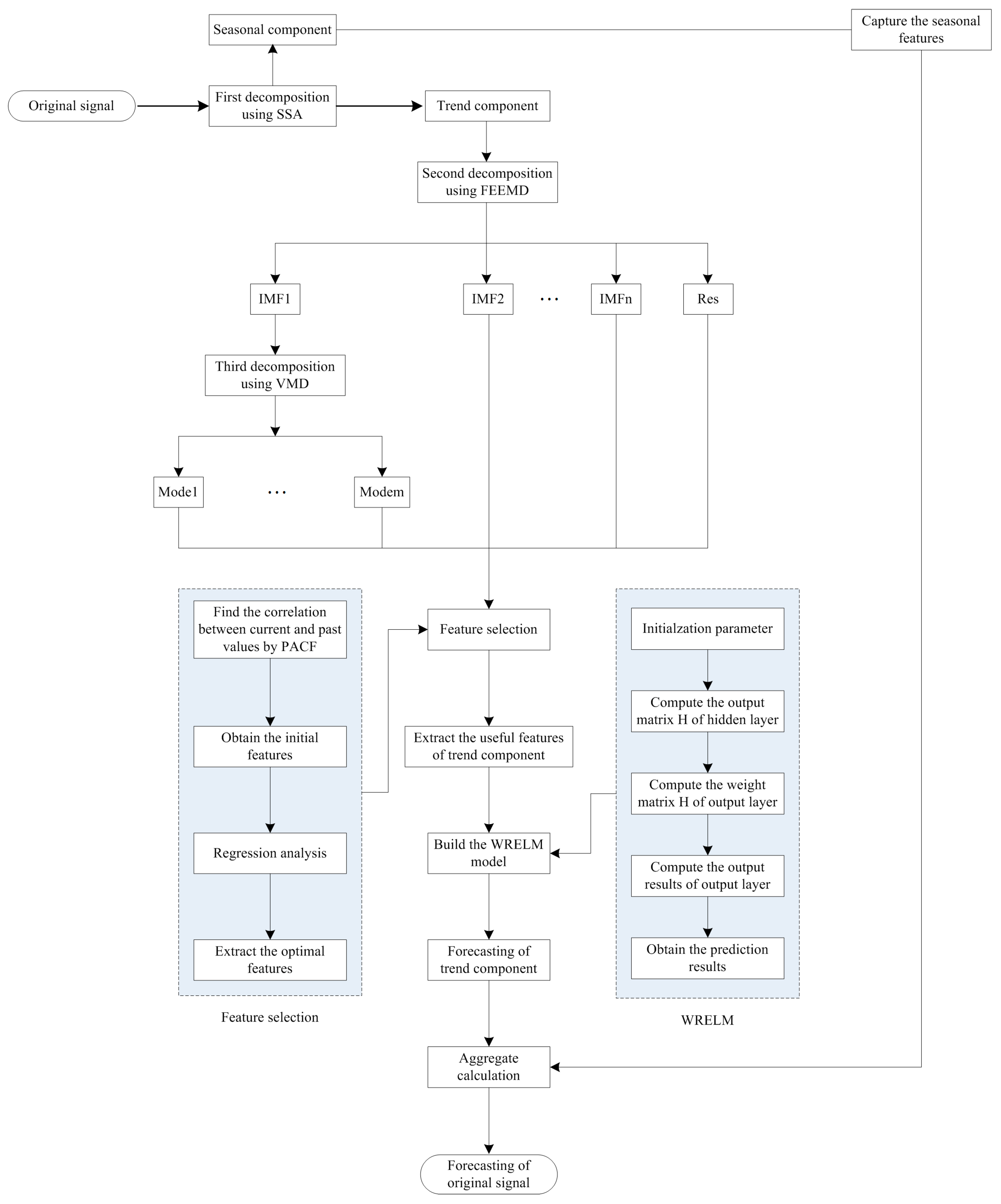
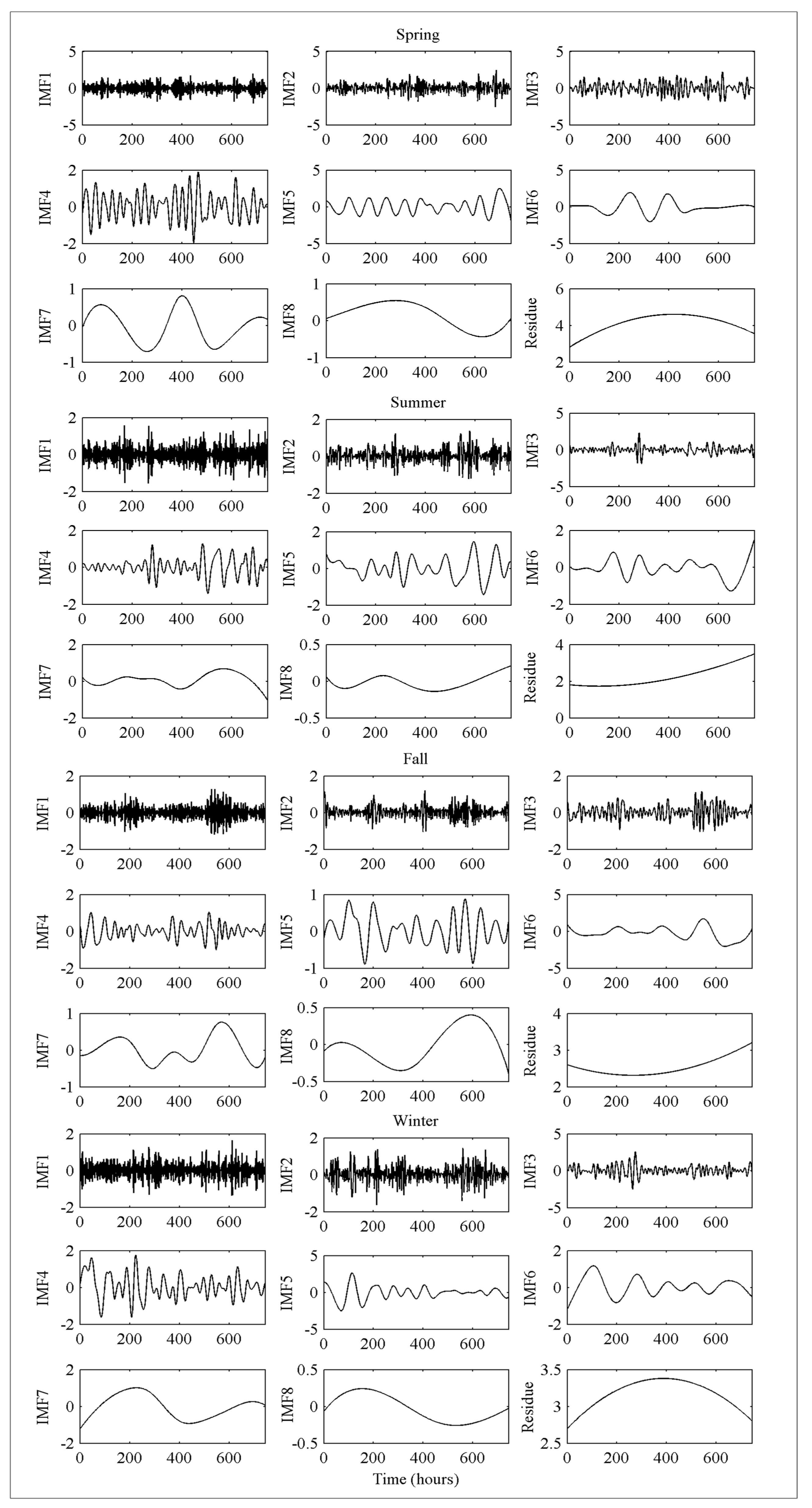
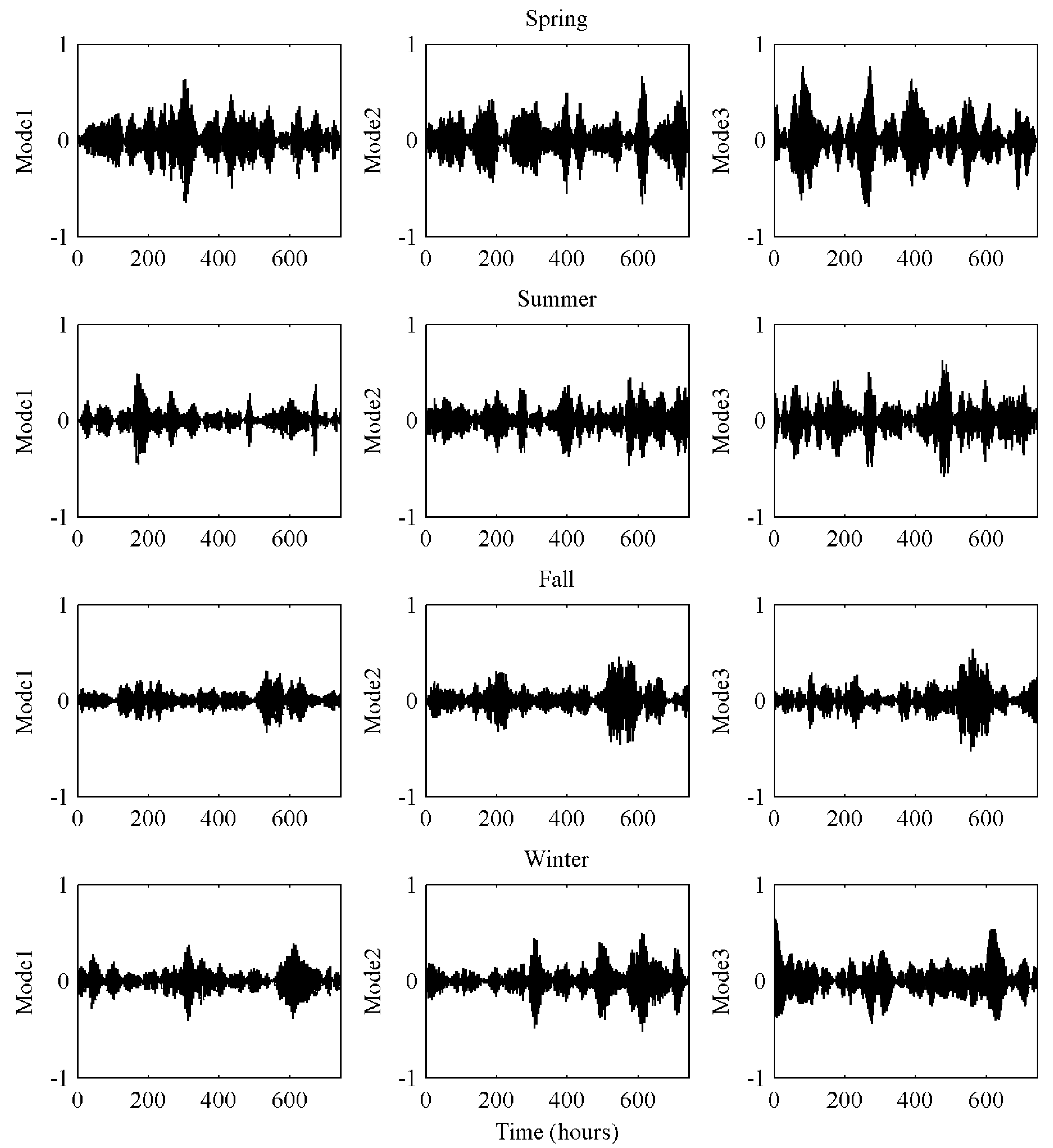
- In order to capture the useful features of wind speed signal and obtain the optimal input-output sample pairs, this study proposes a novel feature extraction framework including three signal decomposition processes of SSA, FEEMD and VMD. First, the SSA is employed to separate the season and trend components of wind speed signal, and capture the seasonal features of wind speed fluctuations. Second, the FEEMD is applied to decompose the trend component into lots of intrinsic mode functions (IMFs) and a residual with different frequencies. Considering the negative effect of high frequencies IMFs (especially IMF1) on the prediction accuracy, the VMD is utilized to further decompose the high frequency IMF1 into several stationary modes for reducing the non-stationarity of the high frequency signal. Finally, a feature selection process is used to capture the useful features of wind speed fluctuations and determine the optimal inputs of the prediction models.
- (4)
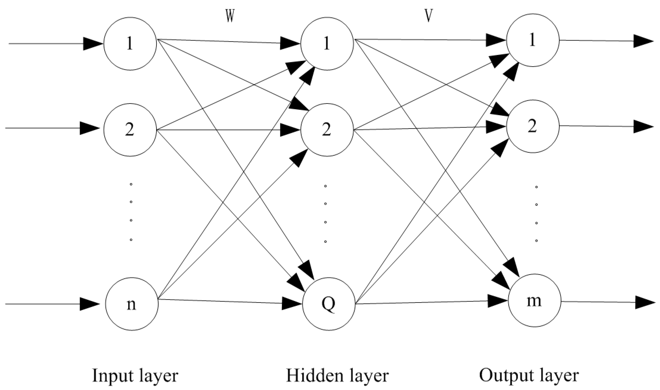
- In order to avoid the over-fitting limitation and reduce the influence of outliers, an improved ELM named WRELM is employed as a basic predictor for building the prediction model by using these selected features.
2. Related Methodology
2.1. Seasonal Separation Algorithm (SSA)
2.2. Fast Ensemble Empirical Mode Decomposition (FEEMD)
2.3. Variational Mode Decomposition (VMD)
2.4. Partial Autocorrelation Function (PACF)
2.5. Weighted Regularized Extreme Learning Machine (WRELM)
2.5.1. Extreme Learning Machine (ELM)
2.5.2. Weighted Regularized Extreme Learning Machine (WRELM)
3. Proposed Approach and Error Criteria
3.1. The Framework of the Proposed Model
- (1)
- Develop a TPSD framework to handle the complex and irregular natures of wind speed signal comprehensively. In the first phase, the SSA is employed to separate the season and trend components of wind speed signal, and capture the seasonal features of wind speed fluctuations. In the second phase, the FEEMD is applied to decompose the trend component into lots of intrinsic mode functions (IMFs) and a residual with different frequencies. Considering the negative effect of high frequencies IMFs (especially IMF1) on the prediction accuracy, the VMD is utilized to further decompose the high frequency IMF1 into several stationary modes for reducing the non-stationarity of the high frequency signal in the third phase. The full dimensions features of wind speed signal can be obtained by TPSD.
- (2)
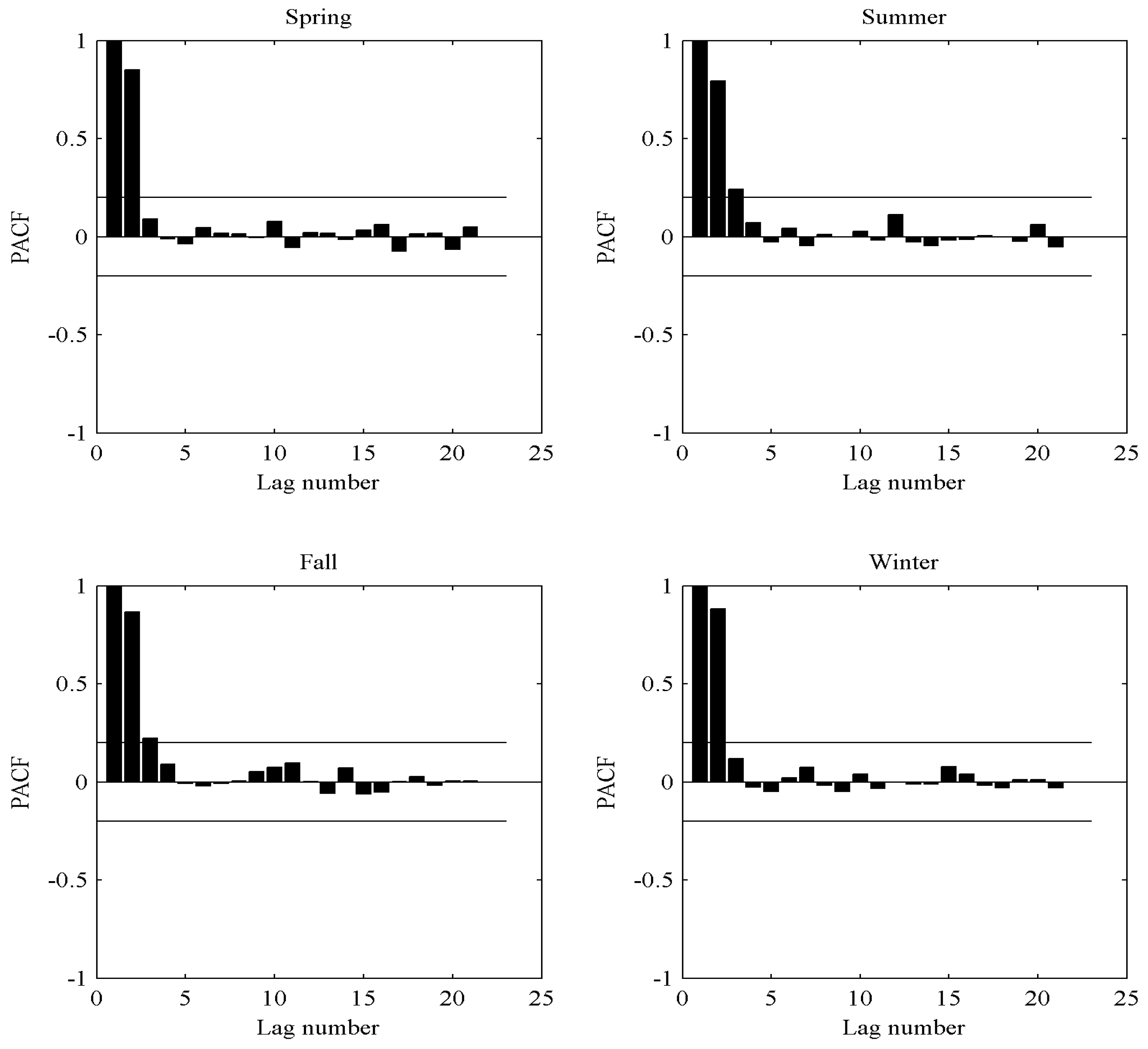
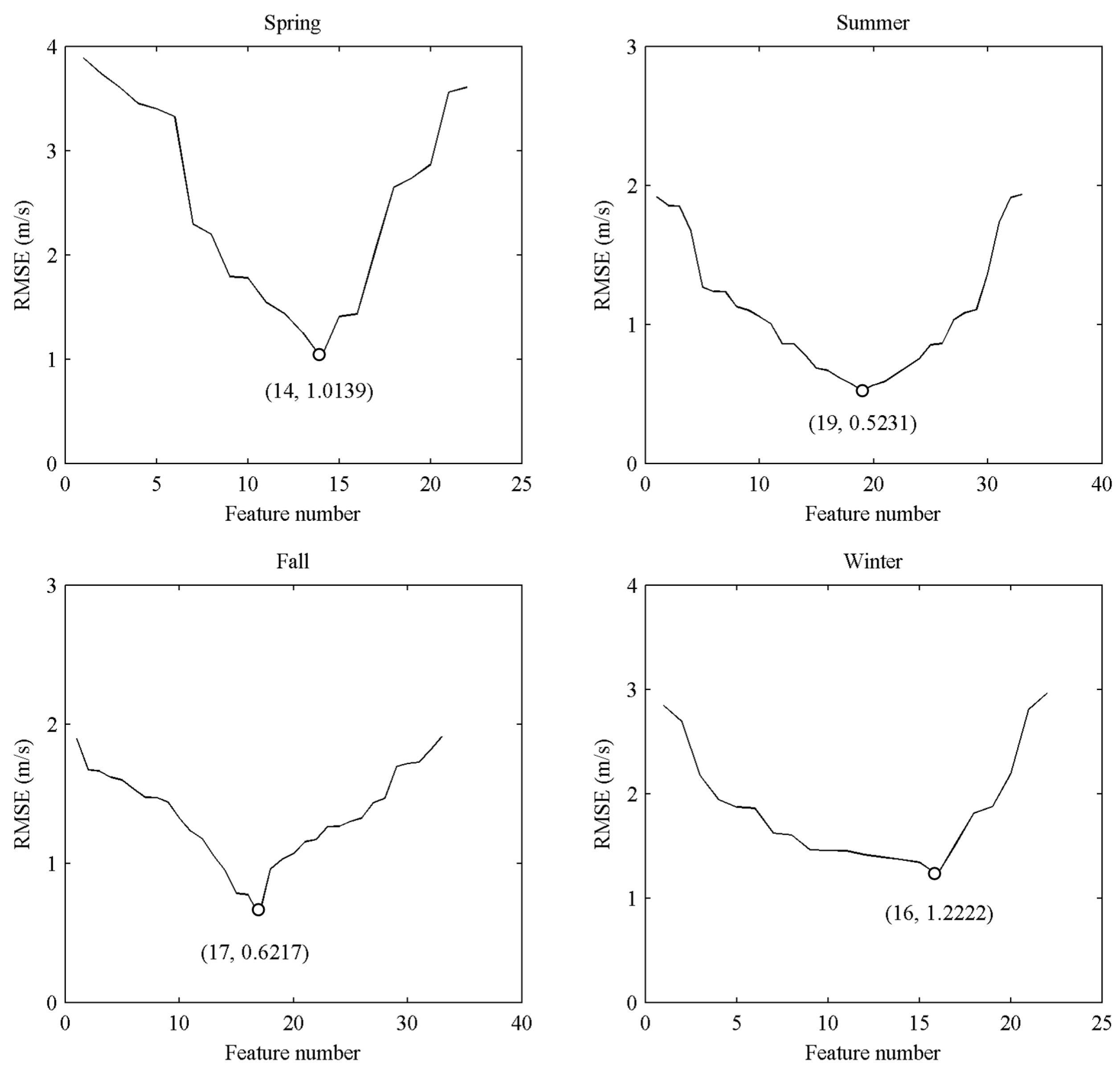
- Propose a feature extraction process to capture the useful features of wind speed fluctuations and determine the optimal features for a prediction model. The PACF is first applied to find the correlation between the current values and the past values of wind speed variable, and determine the initial features for the prediction model. In order to avoid over-fitting, a linear regression is further applied to select the optimal features for the prediction models. In the modeling process of linear regression, the top 80% of training data is called as the learning set which is applied to calculate the parameters of the model, and the remaining 20% of training data is called validation set which is applied to estimate the performance of the model. If one kind of feature combinations can generate the smallest validation error, then the corresponding feature combination is selected as the optimal input features subset for the prediction model.
- (3)
- Use these optimal features to build a WRELM prediction model. Different from the traditional signal decomposition-based prediction models which build a prediction model for each sub-series decomposed from original signal by signal decomposition algorithm, this study only constructs a prediction model using these selected optimal features for saving computation time and improving the prediction accuracy.
3.2. Evaluation Criteria
4. Experimental Simulation
4.1. Data Collection
4.2. Three-Phase Signal Decomposition of Wind Speed Signal
4.3. Feature Selection Process of Trend Components Signal
4.3.1. The Initial Feature Selection Process of Training Samples Using PACF
4.3.2. The Optimal Feature Selection Process of Training Samples Using Regression Analysis
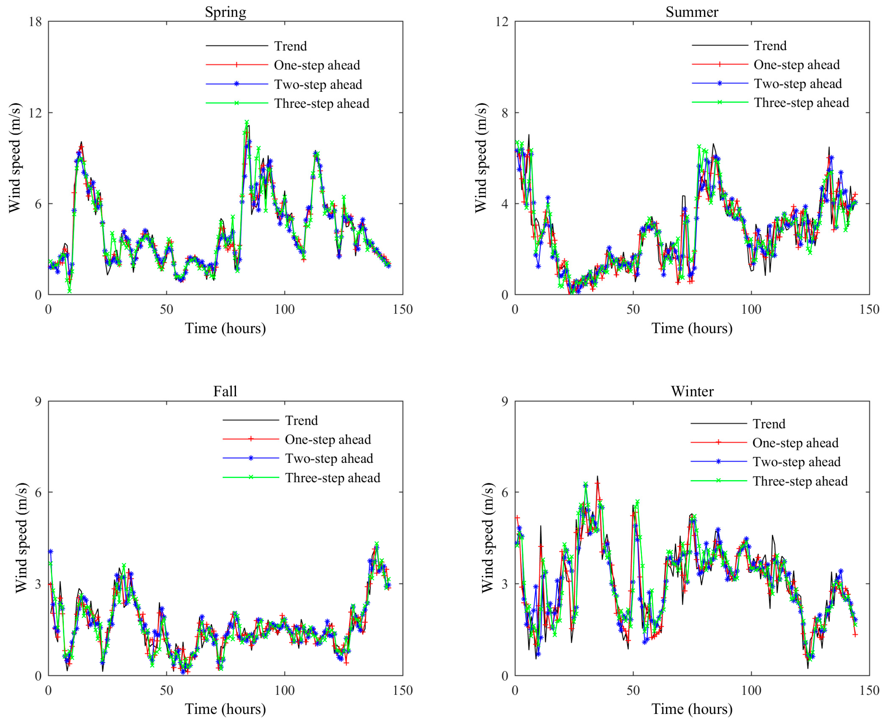
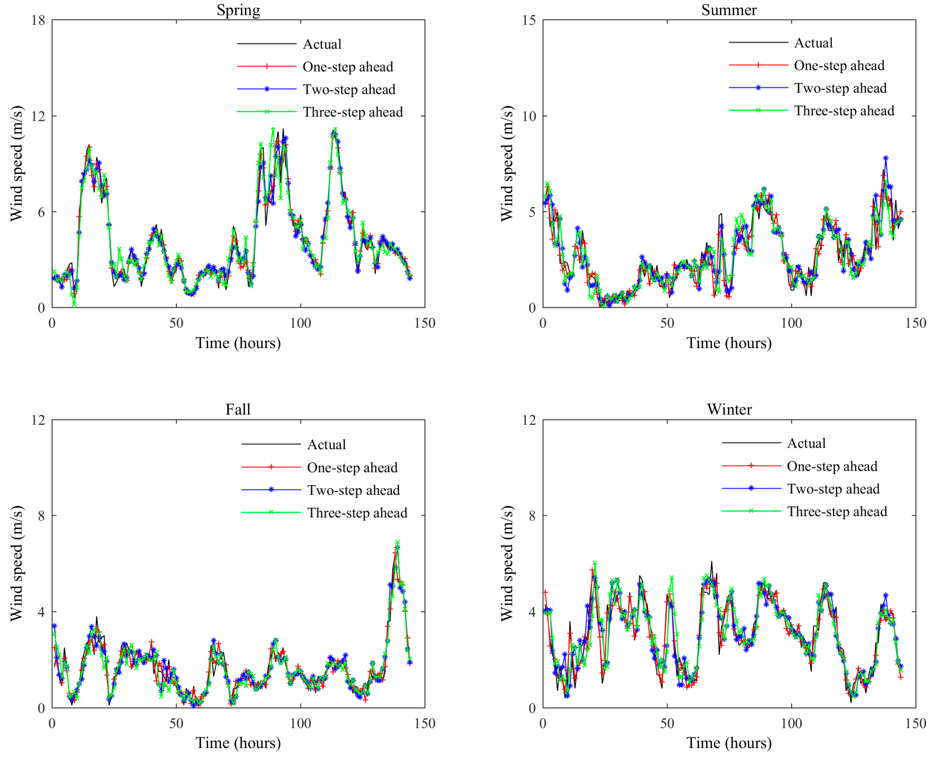
4.4. The Prediction Results of Original Wind Speed Signal
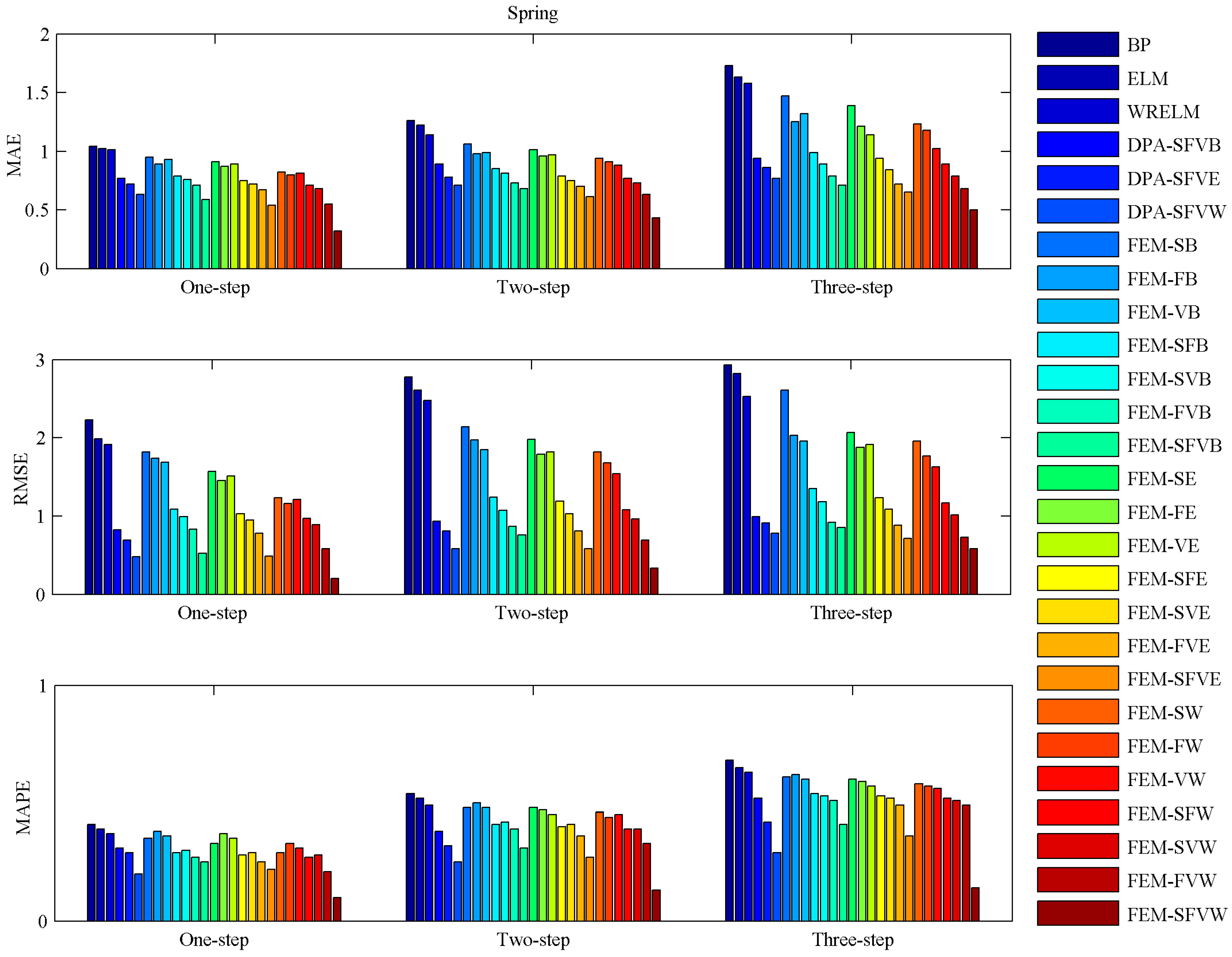
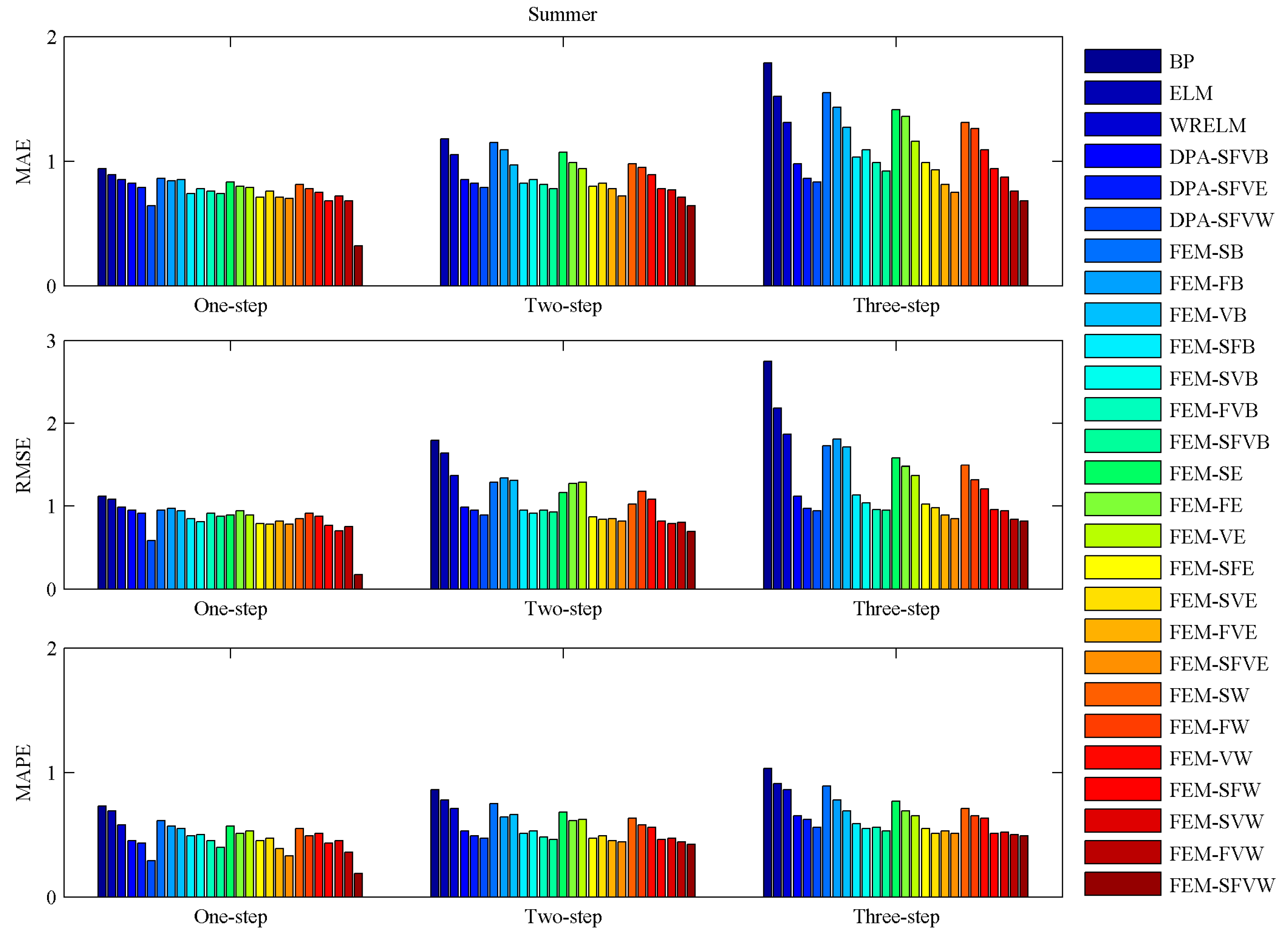
4.5. Model Comparisons
5. Conclusions
Acknowledgments
Author Contributions
Conflicts of Interest
Abbreviations
| SSA | Seasonal Separation Algorithm |
| FEEMD | Fast Ensemble Empirical Mode Decomposition |
| VMD | Variational Mode Decomposition |
| DPA | Decomposition Prediction Aggregation |
| TPSD | Three-Phase Signal Decomposition |
| FEM | Feature Extraction Method |
| PACF | Partial Autocorrelation Function |
| BP | Back Propagation Neural Network |
| ELM | Extreme Learning Machine |
| WRELM | Weighted Regularized Extreme Learning Machine |
| DPA-SFVB | The Common Decomposition Prediction Aggregation-based Hybrid Model of Seasonal Separation Algorithm, Fast Ensemble Empirical Mode Decomposition, Variational Mode Decomposition and Back Propagation Neural Network |
| DPA-SFVE | The Common Decomposition Prediction Aggregation-based Hybrid Model of Seasonal Separation Algorithm, Fast Ensemble Empirical Mode Decomposition, Variational Mode Decomposition and Extreme Learning Machine |
| DPA-SFVW | The Common Decomposition Prediction Aggregation-based Hybrid Model of Seasonal Separation Algorithm, Fast Ensemble Empirical Mode Decomposition, Variational Mode Decomposition and Weighted Regularized Extreme Learning Machine |
| FEM-SB | The Feature Extraction Method-based Hybrid Model of Seasonal Separation Algorithm and Back Propagation Neural Network |
| FEM-FB | The Feature Extraction Method-based Hybrid Model of Fast Ensemble Empirical Mode Decomposition and Back Propagation Neural Network |
| FEM-VB | The Feature Extraction Method-based Hybrid Model of Variational Mode Decomposition and Back Propagation Neural Network |
| FEM-SFB | The Feature Extraction Method-based Hybrid Model of Seasonal Separation Algorithm, Fast Ensemble Empirical Mode Decomposition and Back Propagation Neural Network |
| FEM-SVB | The Feature Extraction Method-based Hybrid Model of Seasonal Separation Algorithm, Variational Mode Decomposition and Back Propagation Neural Network |
| FEM-FVB | The Feature Extraction Method-based Hybrid Model of Fast Ensemble Empirical Mode Decomposition, Variational Mode Decomposition and Back Propagation Neural Network |
| FEM-SFVB | The Feature Extraction Method-based Hybrid Model of Seasonal Separation Algorithm, Fast Ensemble Empirical Mode Decomposition, Variational Mode Decomposition and Back Propagation Neural Network |
| FEM-SE | The Feature Extraction Method-based Hybrid Model of Seasonal Separation Algorithm and Extreme Learning Machine |
| FEM-FE | The Feature Extraction Method-based Hybrid Model of Fast Ensemble Empirical Mode Decomposition and Extreme Learning Machine |
| FEM-VE | The Feature Extraction Method-based Hybrid Model of Variational Mode Decomposition and Extreme Learning Machine |
| FEM-SFE | The Feature Extraction Method-based Hybrid Model of Seasonal Separation Algorithm, Fast Ensemble Empirical Mode Decomposition and Extreme Learning Machine |
| FEM-SVE | The Feature Extraction Method-based Hybrid Model of Seasonal Separation Algorithm, Variational Mode Decomposition and Extreme Learning Machine |
| FEM-FVE | The Feature Extraction Method-based Hybrid Model of Fast Ensemble Empirical Mode Decomposition, Variational Mode Decomposition and Extreme Learning Machine |
| FEM-SFVE | The Feature Extraction Method-based Hybrid Model of Seasonal Separation Algorithm, Fast Ensemble Empirical Mode Decomposition, Variational Mode Decomposition and Extreme Learning Machine |
| FEM-SW | The Feature Extraction Method-based Hybrid Model of Seasonal Separation Algorithm and Weighted Regularized Extreme Learning Machine |
| FEM-FW | The Feature Extraction Method-based Hybrid Model of Fast Ensemble Empirical Mode Decomposition and Weighted Regularized Extreme Learning Machine |
| FEM-VW | The Feature Extraction Method-based Hybrid Model of Variational Mode Decomposition and Weighted Regularized Extreme Learning Machine |
| FEM-SFW | The Feature Extraction Method-based Hybrid Model of Seasonal Separation Algorithm, Fast Ensemble Empirical Mode Decomposition and Weighted Regularized Extreme Learning Machine |
| FEM-SVW | The Feature Extraction Method-based Hybrid Model of Seasonal Separation Algorithm, Variational Mode Decomposition and Weighted Regularized Extreme Learning Machine |
| FEM-FVW | The Feature Extraction Method-based Hybrid Model of Fast Ensemble Empirical Mode Decomposition, Variational Mode Decomposition and Weighted Regularized Extreme Learning Machine |
| FEM-SFVW | The Feature Extraction Method-based Hybrid Model of Seasonal Separation Algorithm, Fast Ensemble Empirical Mode Decomposition, Variational Mode Decomposition and Weighted Regularized Extreme Learning Machine |
| MAE | Mean Absolute Error |
| RMSE | Root Mean Square Error |
| MAPE | Mean Absolute Percentage Error |
References
- Ma, X.J.; Jin, Y.; Dong, Q.L. A generalized dynamic fuzzy neural network based on singular spectrum analysis optimized by brain storm optimization for short-term wind speed forecasting. Appl. Soft Comput. 2017, 54, 296–312. [Google Scholar] [CrossRef]
- Chang, G.W.; Lu, H.J.; Chang, Y.R.; Lee, Y.D. An improved neural network-based approach for short-term wind speed and power forecast. Renew. Energy 2017, 105, 301–311. [Google Scholar] [CrossRef]
- Calif, R.; Schmitt, F.G.; Huang, Y. The multifractal description of wind power fluctuations using arbitrary order Hilbert spectral analysis. Physica A 2013, 392, 4106–4120. [Google Scholar] [CrossRef]
- Calif, R.; Schmitt, F.G. Modeling of atmospheric wind speed sequence using a lognormal stochastic equation. J. Wind Eng. Ind. Aerodyn. 2012, 109, 1–8. [Google Scholar] [CrossRef]
- Calif, R.; Schmitt, F.G. Multiscaling and joint multiscaling description of the atmospheric wind speed and the aggregate power output from a wind farm. Nonlinear Processes Geophys. 2014, 21, 379–392. [Google Scholar] [CrossRef] [Green Version]
- Liu, J.Q.; Wang, X.R.; Lu, Y. A novel hybrid methodology for short-term wind power forecasting based on adaptive neuro-fuzzy inference system. Renew. Energy 2017, 103, 620–629. [Google Scholar] [CrossRef]
- Wang, C.; Zhang, H.L.; Fan, W.H.; Fan, X.C. A new wind power prediction method based on chaotic theory and Bernstein Neural Network. Energy 2016, 117, 259–271. [Google Scholar] [CrossRef]
- Weron, R. Electricity price forecasting: A review of the state-of-the-art with a look into the future. Int. J. Forecast. 2014, 30, 1030–1081. [Google Scholar] [CrossRef]
- Jung, J.; Broadwater, R.P. Current status and future advances for wind speed and power forecasting. Renew. Sustain. Energy Rev. 2014, 31, 762–777. [Google Scholar] [CrossRef]
- Cassola, F.; Burlando, M. Wind speed and wind energy forecast through Kalman filtering of numerical weather prediction model output. Appl. Energy 2012, 99, 154–166. [Google Scholar] [CrossRef]
- Wu, Q.L.; Peng, C.Y. A Least Squares Support Vector Machine Optimized by Cloud-Based Evolutionary Algorithm for Wind Power Generation Prediction. Energies 2016, 9, 585. [Google Scholar] [CrossRef]
- Hu, Q.; Su, P.; Yu, D.; Liu, J. Pattern-based wind speed prediction based on generalized principal component analysis. IEEE Trans. Sustain. Energy 2014, 5, 866–874. [Google Scholar] [CrossRef]
- Erdem, E.; Shi, J. ARMA based approaches for forecasting the tuple of wind speed and direction. Appl. Energy 2011, 88, 1405–1414. [Google Scholar] [CrossRef]
- Bivona, S.; Bonanno, G.; Burlon, R.; Gurrera, D.; Leone, C. Stochastic models for wind speed forecasting. Energy Convers. Manag. 2011, 52, 1157–1165. [Google Scholar] [CrossRef]
- Shamshad, A.; Bawadi, M.A.; Hussin, W.M.A.W.; Majid, T.A.; Sanusi, S.A.M. First and second order Markov chain models for synthetic generation of wind speed time series. Energy 2005, 30, 693–708. [Google Scholar] [CrossRef]
- Torres, J.L.; Garcia, A.; De Blas, M.; De Francisco, A. Forecast of hourly average wind speed with Arma models in Navarre (Spain). Sol. Energy 2005, 79, 65–77. [Google Scholar] [CrossRef]
- Louka, P.; Galanis, G.; Siebert, N.; Kariniotakis, G.; Katsafados, P.; Pytharoulis, I.; Kallos, G. Improvements in wind speed forecasts for wind power prediction purposes using Kalman filtering. J. Wind Eng. Ind. Aerodyn. 2008, 96, 2348–2362. [Google Scholar] [CrossRef] [Green Version]
- Yu, J.; Chen, K.; Mori, J.; Rashid, M.M. A Gaussian mixture copula model based localized Gaussian process regression approach for long-term wind speed prediction. Energy 2013, 61, 673–686. [Google Scholar] [CrossRef]
- Guo, Z.H.; Zhao, J.; Zhang, W.Y.; Wang, J.Z. A corrected hybrid approach for wind speed prediction in Hexi Corridor of China. Energy 2011, 36, 1668–1679. [Google Scholar] [CrossRef]
- Liu, H.; Shi, J.; Erdem, E. Prediction of wind speed time series using modified Taylor Kriging method. Energy 2010, 35, 4870–4879. [Google Scholar] [CrossRef]
- Wang, J.Z.; Qin, S.S.; Zhou, Q.P.; Jiang, H.Y. Medium-term wind speeds forecasting utilizing hybrid models for three different sites in Xinjiang, China. Renew. Energy 2015, 76, 91–101. [Google Scholar] [CrossRef]
- Velo, R.; López, P.; Maseda, F. Wind speed estimation using multilayer perceptron. Energy Convers. Manag. 2014, 81, 1–9. [Google Scholar] [CrossRef]
- Shamshirband, S.; Petkovic, D.; Amini, A.; Anuar, N.B.; Nikolic, V.; Cojbasic, Z.; Kiah, L.M.; Gani, A. Support vector regression methodology for wind turbine reaction torque prediction with power-split hydrostatic continuous variable transmission. Energy 2014, 67, 623–630. [Google Scholar] [CrossRef]
- Li, G.; Shi, J. On comparing three artificial neural networks for wind speed forecasting. Appl. Energy 2010, 87, 2313–2320. [Google Scholar] [CrossRef]
- Zhou, J.; Shi, J.; Li, G. Fine tuning support vector machines for short-term wind speed forecasting. Energy Convers. Manag. 2011, 52, 1990–1998. [Google Scholar] [CrossRef]
- Cincotti, S.; Gallo, G.; Ponta, L.; Raberto, M. Modelling and forecasting of electricity spot-prices: Computational intelligence vs classical econometrics. AI Commun. 2014, 27, 301–314. [Google Scholar]
- Shi, J.; Guo, J.M.; Zheng, S.Y. Evaluation of hybrid forecasting approaches for wind speed and power generation time series. Renew. Sustain. Energy Rev. 2012, 16, 3471–3480. [Google Scholar] [CrossRef]
- Wang, J.Z.; Hu, J.M.; Ma, K.L.; Zhang, Y.X. A self-adaptive hybrid approach for wind speed forecasting. Renew. Energy 2015, 78, 374–385. [Google Scholar] [CrossRef]
- Khashei, M.; Bijari, M.; Ardali, G.A.R. Improvement of auto-regressive integrated moving average models using fuzzy logic and artificial neural networks (ANNs). Neurocomputing 2009, 72, 956–967. [Google Scholar] [CrossRef]
- Kani, S.P.; Ardehali, M. Very short-term wind speed prediction: A new artificial neural network-Markov chain model. Energy Convers. Manag. 2011, 52, 738–745. [Google Scholar] [CrossRef]
- De Giorgi, M.G.; Congedo, P.M.; Malvoni, M.; Laforgia, D. Error analysis of hybrid photovoltaic power forecasting models: A case study of Mediterranean climate. Energy Convers. Manag. 2015, 100, 117–130. [Google Scholar] [CrossRef]
- Ren, Y.; Suganthan, P.; Srikanth, N. A comparative study of empirical mode decomposition-based short-term wind speed forecasting methods. IEEE Trans. Sustain. Energy 2015, 6, 236–244. [Google Scholar] [CrossRef]
- Liu, H.; Chen, C.; Tian, H.Q.; Li, Y.F. A hybrid model for wind speed prediction using empirical mode decomposition and artificial neural networks. Renew. Energy 2012, 48, 545–556. [Google Scholar] [CrossRef]
- Zhang, G.P.; Qi, M. Neural network forecasting for seasonal and trend time series. Eur. J. Oper. Res. 2005, 160, 501–514. [Google Scholar] [CrossRef]
- Guo, Z.H.; Wu, J.; Lu, H.Y.; Wang, J.Z. A case study on a hybrid wind speed forecasting method using BP neural network. Knowl. Based Syst. 2011, 24, 1048–1056. [Google Scholar] [CrossRef]
- Wu, Z.; Huang, N.E. Ensemble empirical mode decomposition: A noise assisted data analysis method. Adv. Adapt. Data Anal. 2008, 1, 1–41. [Google Scholar] [CrossRef]
- Wang, Y.H.; Yeh, C.H.; Young, H.W.V.; Hu, K.; Lo, M.T. On the computational complexity of the empirical mode decomposition algorithm. Phys. A Stat. Mech. Appl. 2014, 400, 159–167. [Google Scholar] [CrossRef]
- Liu, H.; Tian, H.Q.; Li, Y.F. Comparison of new hybrid FEEMD-MLP, FEEMD-ANFIS, wavelet packet-MLP and wavelet packet-ANFIS for wind speed predictions. Energy Convers. Manag. 2005, 89, 1–11. [Google Scholar] [CrossRef]
- Dragomiretskiy, K.; Zosso, D. Variational mode decomposition. IEEE Trans. Signal Process. 2014, 62, 531–544. [Google Scholar] [CrossRef]
- Abdoos, A.A. A new intelligent method based on combination of VMD and ELM for short term wind power forecasting. Neurocomputing 2016, 203, 111–120. [Google Scholar] [CrossRef]
- Wang, H.; Zhao, W. ARIMA model estimated by Particle Swarm optimization algorithm for Consumer price index forecasting, Lecture notes in computer Science. Artif. Intell. Comput. Intell. 2009, 5855, 48–58. [Google Scholar]
- Guo, Z.H.; Zhao, W.G.; Lu, H.Y.; Wang, J.Z. Multi-step forecasting for wind speed using a modified EMD-based artificial neural network model. Renew. Energy 2012, 37, 241–249. [Google Scholar] [CrossRef]
- Huang, G.B.; Zhu, Q.Y.; Siew, C.K. Extreme learning machine: Theory and applications. Neurocomputing 2006, 70, 489–501. [Google Scholar] [CrossRef]
- Huang, G.B.; Zhou, H.; Ding, X.; Zhang, R. Extreme learning machine for regression and multiclass classification. IEEE Trans. Syst. Man Cybern. Part B 2012, 42, 513–529. [Google Scholar] [CrossRef] [PubMed]
- Liu, H.; Tian, H.Q.; Li, Y.F. Four wind speed multi-step forecasting models using extreme learning machines and signal decomposing algorithms. Energy Convers. Manag. 2015, 100, 16–22. [Google Scholar] [CrossRef]
- Martínez-Martínez, J.M.; Escandell-Montero, P.; Soria-Olivas, E.; Martín-Guerrero, J.D.; Magdalena-Benedito, R.; Gómez-Sanchis, J. Regularized extreme learning machine for regression problems. Neurocomputing 2011, 74, 3716–3721. [Google Scholar] [CrossRef]
- Zhang, K.; Luo, M. Outlier-robust extreme learning machine for regression problems. Neurocomputing 2015, 151, 1519–1527. [Google Scholar] [CrossRef]
| Cases | Mean (m/s) | Std.dev (m/s) | Maximum (m/s) | Median (m/s) | Minimum (m/s) |
|---|---|---|---|---|---|
| Spring | 4.24 | 2.39 | 13.40 | 3.75 | 0.50 |
| Summer | 2.20 | 1.55 | 10.80 | 1.80 | 0.10 |
| Fall | 2.23 | 1.47 | 8.60 | 1.80 | 0.10 |
| Winter | 3.13 | 1.83 | 9.70 | 2.90 | 0.10 |
| Times | Datasets | Times | Datasets | ||||||
|---|---|---|---|---|---|---|---|---|---|
| Spring | Summer | Fall | Winter | Spring | Summer | Fall | Winter | ||
| 1 | 1.02 | 0.86 | 0.84 | 0.93 | 13 | 0.90 | 0.88 | 0.81 | 0.74 |
| 2 | 0.96 | 1.03 | 0.90 | 0.84 | 14 | 0.97 | 0.97 | 0.98 | 0.80 |
| 3 | 0.90 | 0.92 | 0.88 | 0.89 | 15 | 1.14 | 1.12 | 1.17 | 1.19 |
| 4 | 0.85 | 0.88 | 0.83 | 0.95 | 16 | 1.13 | 1.28 | 1.37 | 1.29 |
| 5 | 0.82 | 0.84 | 0.81 | 0.86 | 17 | 1.17 | 1.41 | 1.46 | 1.34 |
| 6 | 0.85 | 0.71 | 0.77 | 0.85 | 18 | 1.22 | 1.45 | 1.56 | 1.37 |
| 7 | 0.80 | 0.75 | 0.74 | 0.88 | 19 | 1.22 | 1.41 | 1.60 | 1.46 |
| 8 | 0.87 | 0.76 | 0.72 | 0.80 | 20 | 1.24 | 1.38 | 1.47 | 1.42 |
| 9 | 0.86 | 0.72 | 0.82 | 0.76 | 21 | 1.22 | 1.18 | 1.38 | 1.41 |
| 10 | 0.83 | 0.73 | 0.69 | 0.68 | 22 | 1.20 | 1.17 | 1.24 | 1.23 |
| 11 | 0.85 | 0.69 | 0.71 | 0.73 | 23 | 1.09 | 1.11 | 0.84 | 0.95 |
| 12 | 0.90 | 0.62 | 0.78 | 0.69 | 24 | 0.98 | 1.13 | 0.64 | 0.94 |
| Cases | Initial Features |
|---|---|
| Spring | TC(t), TC(t − 1) |
| Summer | TC(t), TC(t − 1), TC(t − 2) |
| Fall | TC(t), TC(t − 1), TC(t − 2) |
| Winter | TC(t), TC(t − 1) |
| Cases | Initial Features |
|---|---|
| Spring | IMF2(t), IMF3(t), IMF4(t), IMF5(t), IMF6(t), IMF7(t), IMF8(t), Residue(t), Mode1(t), Mode2(t), Mode3(t), IMF2(t − 1), IMF3(t − 1), IMF4(t − 1), IMF5(t − 1), IMF6(t − 1), IMF7(t − 1), IMF8(t − 1), Residue(t − 1), Mode1(t − 1), Mode2(t − 1), Mode3(t − 1) |
| Summer | IMF2(t), IMF3(t), IMF4(t), IMF5(t), IMF6(t), IMF7(t), IMF8(t), Residue(t), Mode1(t), Mode2(t), Mode3(t), IMF2(t − 1), IMF3(t − 1), IMF4(t − 1), IMF5(t − 1), IMF6(t − 1), IMF7(t − 1), IMF8(t − 1), Residue(t − 1), Mode1(t − 1), Mode2(t − 1), Mode3(t − 1), IMF2(t − 2), IMF3(t − 2), IMF4(t − 2), IMF5(t − 2), IMF6(t − 2), IMF7(t − 2), IMF8(t − 2), Residue(t − 2), Mode1(t − 2), Mode2(t − 2), Mode3(t − 2) |
| Fall | IMF2(t), IMF3(t), IMF4(t), IMF5(t), IMF6(t), IMF7(t), IMF8(t), Residue(t), Mode1(t), Mode2(t), Mode3(t), IMF2(t − 1), IMF3(t − 1), IMF4(t − 1), IMF5(t − 1), IMF6(t − 1), IMF7(t − 1), IMF8(t − 1), Residue(t − 1), Mode1(t − 1), Mode2(t − 1), Mode3(t − 1), IMF2(t − 2), IMF3(t − 2), IMF4(t − 2), IMF5(t − 2), IMF6(t − 2), IMF7(t − 2), IMF8(t − 2), Residue(t − 2), Mode1(t − 2), Mode2(t − 2), Mode3(t − 2) |
| Winter | IMF2(t), IMF3(t), IMF4(t), IMF5(t), IMF6(t), IMF7(t), IMF8(t), Residue(t), Mode1(t), Mode2(t), Mode3(t), IMF2(t − 1), IMF3(t − 1), IMF4(t − 1), IMF5(t − 1), IMF6(t − 1), IMF7(t − 1), IMF8(t − 1), Residue(t − 1), Mode1(t − 1), Mode2(t − 1), Mode3(t − 1) |
| Cases | Optimal Features |
|---|---|
| Spring | IMF2(t), IMF3(t), IMF4(t), IMF5(t), IMF6(t), IMF7(t), IMF8(t), Residue(t), Mode1(t), Mode2(t), Mode3(t), IMF2(t − 1) , IMF3(t − 1), IMF4(t − 1) |
| Summer | IMF2(t), IMF3(t), IMF4(t), IMF5(t), IMF6(t), IMF7(t), IMF8(t), Residue(t), Mode1(t), Mode2(t), Mode3(t), IMF2(t − 1), IMF3(t − 1), IMF4(t − 1), IMF5(t − 1), IMF6(t − 1), IMF7(t − 1), IMF8(t − 1), Residue(t − 1) |
| Fall | IMF2(t), IMF3(t), IMF4(t), IMF5(t), IMF6(t), IMF7(t), IMF8(t), Residue(t), Mode1(t), Mode2(t), Mode3(t), IMF2(t − 1), IMF3(t − 1), IMF4(t − 1), IMF5(t − 1), IMF6(t − 1), IMF7(t − 1) |
| Winter | IMF2(t), IMF3(t), IMF4(t), IMF5(t), IMF6(t), IMF7(t), IMF8(t), Residue(t), Mode1(t), Mode2(t), Mode3(t), IMF2(t − 1), IMF3(t − 1), IMF4(t − 1), IMF5(t − 1), IMF6(t − 1) |
| Categories | Models | Spring | ||||||||
|---|---|---|---|---|---|---|---|---|---|---|
| One-Step Ahead | Two-Step Ahead | Three-Step Ahead | ||||||||
| MAE | RMSE | MAPE | MAE | RMSE | MAPE | MAE | RMSE | MAPE | ||
| Single | BP | 1.04 | 2.23 | 0.41 | 1.26 | 2.78 | 0.54 | 1.73 | 2.93 | 0.68 |
| ELM | 1.02 | 1.99 | 0.39 | 1.22 | 2.61 | 0.52 | 1.63 | 2.82 | 0.65 | |
| WRELM | 1.01 | 1.91 | 0.37 | 1.14 | 2.48 | 0.49 | 1.58 | 2.53 | 0.63 | |
| DPA | DPA-SFVB | 0.77 | 0.82 | 0.31 | 0.89 | 0.93 | 0.38 | 0.94 | 0.99 | 0.52 |
| DPA-SFVE | 0.72 | 0.69 | 0.29 | 0.78 | 0.81 | 0.32 | 0.86 | 0.91 | 0.42 | |
| DPA-SFVW | 0.63 | 0.48 | 0.20 | 0.71 | 0.58 | 0.25 | 0.77 | 0.78 | 0.29 | |
| FEM | FEM-SB | 0.95 | 1.82 | 0.35 | 1.06 | 2.14 | 0.48 | 1.47 | 2.61 | 0.61 |
| FEM-FB | 0.89 | 1.74 | 0.38 | 0.98 | 1.97 | 0.50 | 1.25 | 2.03 | 0.62 | |
| FEM-VB | 0.93 | 1.69 | 0.36 | 0.99 | 1.85 | 0.48 | 1.32 | 1.96 | 0.60 | |
| FEM-SFB | 0.79 | 1.09 | 0.29 | 0.85 | 1.24 | 0.41 | 0.99 | 1.35 | 0.54 | |
| FEM-SVB | 0.76 | 0.99 | 0.30 | 0.81 | 1.07 | 0.42 | 0.89 | 1.18 | 0.53 | |
| FEM-FVB | 0.71 | 0.83 | 0.27 | 0.73 | 0.87 | 0.39 | 0.79 | 0.92 | 0.51 | |
| FEM-SFVB | 0.59 | 0.52 | 0.25 | 0.68 | 0.76 | 0.31 | 0.71 | 0.85 | 0.41 | |
| FEM-SE | 0.91 | 1.57 | 0.33 | 1.01 | 1.98 | 0.48 | 1.39 | 2.07 | 0.60 | |
| FEM-FE | 0.87 | 1.45 | 0.37 | 0.96 | 1.79 | 0.47 | 1.21 | 1.88 | 0.59 | |
| FEM-VE | 0.89 | 1.51 | 0.35 | 0.97 | 1.82 | 0.45 | 1.14 | 1.91 | 0.57 | |
| FEM-SFE | 0.75 | 1.03 | 0.28 | 0.79 | 1.19 | 0.40 | 0.94 | 1.23 | 0.53 | |
| FEM-SVE | 0.72 | 0.95 | 0.29 | 0.75 | 1.03 | 0.41 | 0.84 | 1.09 | 0.52 | |
| FEM-FVE | 0.67 | 0.78 | 0.25 | 0.70 | 0.81 | 0.36 | 0.72 | 0.88 | 0.49 | |
| FEM-SFVE | 0.54 | 0.49 | 0.22 | 0.61 | 0.58 | 0.27 | 0.65 | 0.71 | 0.36 | |
| FEM-SW | 0.82 | 1.23 | 0.29 | 0.94 | 1.82 | 0.46 | 1.23 | 1.96 | 0.58 | |
| FEM-FW | 0.80 | 1.16 | 0.33 | 0.91 | 1.68 | 0.44 | 1.18 | 1.77 | 0.57 | |
| FEM-VW | 0.81 | 1.21 | 0.31 | 0.88 | 1.54 | 0.45 | 1.02 | 1.63 | 0.56 | |
| FEM-SFW | 0.71 | 0.97 | 0.27 | 0.77 | 1.08 | 0.39 | 0.89 | 1.17 | 0.52 | |
| FEM-SVW | 0.68 | 0.89 | 0.28 | 0.73 | 0.96 | 0.39 | 0.79 | 1.01 | 0.51 | |
| FEM-FVW | 0.55 | 0.58 | 0.21 | 0.63 | 0.69 | 0.33 | 0.68 | 0.73 | 0.49 | |
| FEM-SFVW | 0.32 | 0.20 | 0.10 | 0.43 | 0.33 | 0.13 | 0.50 | 0.58 | 0.14 | |
| Categories | Models | Summer | ||||||||
|---|---|---|---|---|---|---|---|---|---|---|
| One-Step Ahead | Two-Step Ahead | Three-Step Ahead | ||||||||
| MAE | RMSE | MAPE | MAE | RMSE | MAPE | MAE | RMSE | MAPE | ||
| Single | BP | 0.94 | 1.12 | 0.73 | 1.24 | 1.79 | 0.86 | 1.79 | 2.75 | 1.03 |
| ELM | 0.89 | 1.08 | 0.69 | 1.18 | 1.64 | 0.78 | 1.52 | 2.18 | 0.91 | |
| WRELM | 0.85 | 0.99 | 0.58 | 1.05 | 1.37 | 0.71 | 1.35 | 1.87 | 0.86 | |
| DPA | DPA-SFVB | 0.82 | 0.95 | 0.45 | 0.85 | 0.99 | 0.53 | 0.98 | 1.12 | 0.65 |
| DPA-SFVE | 0.79 | 0.91 | 0.43 | 0.82 | 0.95 | 0.49 | 0.86 | 0.97 | 0.62 | |
| DPA-SFVW | 0.64 | 0.58 | 0.29 | 0.79 | 0.89 | 0.47 | 0.83 | 0.94 | 0.56 | |
| FEM | FEM-SB | 0.86 | 0.95 | 0.61 | 1.15 | 1.29 | 0.75 | 1.55 | 1.73 | 0.89 |
| FEM-FB | 0.84 | 0.97 | 0.57 | 1.09 | 1.34 | 0.64 | 1.43 | 1.81 | 0.78 | |
| FEM-VB | 0.85 | 0.94 | 0.55 | 0.97 | 1.31 | 0.66 | 1.27 | 1.71 | 0.69 | |
| FEM-SFB | 0.74 | 0.89 | 0.49 | 0.82 | 0.95 | 0.51 | 1.03 | 1.13 | 0.59 | |
| FEM-SVB | 0.78 | 0.89 | 0.50 | 0.85 | 0.96 | 0.53 | 1.09 | 1.04 | 0.55 | |
| FEM-FVB | 0.76 | 0.91 | 0.45 | 0.81 | 0.95 | 0.48 | 0.99 | 0.96 | 0.56 | |
| FEM-SFVB | 0.70 | 0.78 | 0.40 | 0.78 | 0.90 | 0.46 | 0.92 | 0.95 | 0.53 | |
| FEM-SE | 0.83 | 0.89 | 0.57 | 1.07 | 1.16 | 0.68 | 1.41 | 1.58 | 0.77 | |
| FEM-FE | 0.80 | 0.94 | 0.51 | 0.99 | 1.27 | 0.61 | 1.36 | 1.48 | 0.69 | |
| FEM-VE | 0.79 | 0.89 | 0.53 | 0.94 | 1.29 | 0.62 | 1.16 | 1.37 | 0.65 | |
| FEM-SFE | 0.71 | 0.79 | 0.45 | 0.80 | 0.87 | 0.47 | 0.99 | 1.02 | 0.55 | |
| FEM-SVE | 0.76 | 0.81 | 0.47 | 0.82 | 0.84 | 0.49 | 0.93 | 0.98 | 0.56 | |
| FEM-FVE | 0.71 | 0.82 | 0.39 | 0.78 | 0.85 | 0.45 | 0.81 | 0.89 | 0.53 | |
| FEM-SFVE | 0.66 | 0.74 | 0.33 | 0.72 | 0.82 | 0.44 | 0.75 | 0.85 | 0.51 | |
| FEM-SW | 0.81 | 0.85 | 0.55 | 0.98 | 1.02 | 0.63 | 1.27 | 1.49 | 0.71 | |
| FEM-FW | 0.78 | 0.91 | 0.49 | 0.95 | 1.18 | 0.58 | 1.26 | 1.32 | 0.65 | |
| FEM-VW | 0.75 | 0.88 | 0.51 | 0.89 | 1.08 | 0.56 | 1.09 | 1.21 | 0.63 | |
| FEM-SFW | 0.68 | 0.77 | 0.43 | 0.78 | 0.82 | 0.46 | 0.94 | 0.96 | 0.51 | |
| FEM-SVW | 0.72 | 0.70 | 0.45 | 0.77 | 0.79 | 0.47 | 0.87 | 0.94 | 0.52 | |
| FEM-FVW | 0.68 | 0.75 | 0.36 | 0.71 | 0.80 | 0.44 | 0.76 | 0.84 | 0.50 | |
| FEM-SFVW | 0.32 | 0.17 | 0.19 | 0.64 | 0.69 | 0.42 | 0.68 | 0.82 | 0.49 | |
| Categories | Models | Fall | ||||||||
|---|---|---|---|---|---|---|---|---|---|---|
| One-Step Ahead | Two-Step Ahead | Three-Step Ahead | ||||||||
| MAE | RMSE | MAPE | MAE | RMSE | MAPE | MAE | RMSE | MAPE | ||
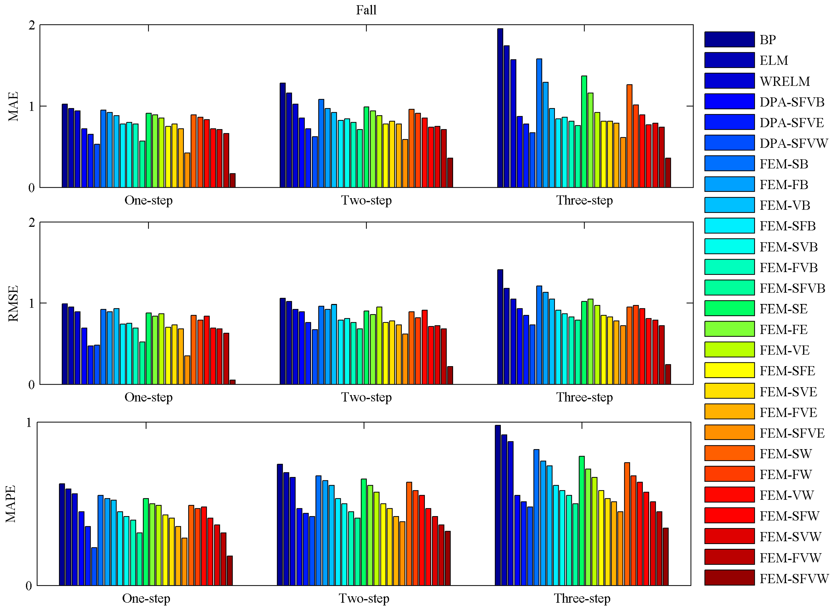
| Single | BP | 1.02 | 0.99 | 0.62 | 1.28 | 1.06 | 0.74 | 1.95 | 1.41 | 0.98 |
| ELM | 0.97 | 0.95 | 0.59 | 1.16 | 1.02 | 0.69 | 1.74 | 1.18 | 0.92 | |
| WRELM | 0.94 | 0.89 | 0.56 | 1.02 | 0.92 | 0.66 | 1.57 | 1.05 | 0.88 | |
| DPA | DPA-SFVB | 0.72 | 0.69 | 0.45 | 0.85 | 0.89 | 0.47 | 0.87 | 0.93 | 0.55 |
| DPA-SFVE | 0.65 | 0.47 | 0.36 | 0.72 | 0.76 | 0.44 | 0.78 | 0.85 | 0.51 | |
| DPA-SFVW | 0.53 | 0.48 | 0.23 | 0.62 | 0.67 | 0.42 | 0.67 | 0.73 | 0.48 | |
| FEM | FEM-SB | 0.95 | 0.92 | 0.55 | 1.08 | 0.96 | 0.67 | 1.58 | 1.21 | 0.83 |
| FEM-FB | 0.92 | 0.89 | 0.53 | 0.97 | 0.92 | 0.64 | 1.29 | 1.13 | 0.76 | |
| FEM-VB | 0.88 | 0.93 | 0.52 | 0.92 | 0.98 | 0.61 | 0.97 | 1.05 | 0.73 | |
| FEM-SFB | 0.78 | 0.74 | 0.45 | 0.82 | 0.79 | 0.53 | 0.84 | 0.91 | 0.61 | |
| FEM-SVB | 0.80 | 0.75 | 0.42 | 0.84 | 0.81 | 0.50 | 0.86 | 0.87 | 0.58 | |
| FEM-FVB | 0.78 | 0.69 | 0.40 | 0.80 | 0.76 | 0.45 | 0.81 | 0.83 | 0.55 | |
| FEM-SFVB | 0.57 | 0.52 | 0.32 | 0.71 | 0.68 | 0.41 | 0.76 | 0.79 | 0.50 | |
| FEM-SE | 0.91 | 0.88 | 0.53 | 0.99 | 0.90 | 0.65 | 1.37 | 1.02 | 0.79 | |
| FEM-FE | 0.89 | 0.84 | 0.50 | 0.94 | 0.86 | 0.61 | 1.16 | 1.05 | 0.71 | |
| FEM-VE | 0.85 | 0.87 | 0.49 | 0.88 | 0.95 | 0.57 | 0.92 | 0.97 | 0.66 | |
| FEM-SFE | 0.75 | 0.70 | 0.43 | 0.78 | 0.76 | 0.50 | 0.81 | 0.85 | 0.58 | |
| FEM-SVE | 0.78 | 0.73 | 0.41 | 0.81 | 0.78 | 0.47 | 0.81 | 0.83 | 0.53 | |
| FEM-FVE | 0.72 | 0.68 | 0.36 | 0.78 | 0.73 | 0.42 | 0.79 | 0.78 | 0.51 | |
| FEM-SFVE | 0.42 | 0.35 | 0.29 | 0.59 | 0.62 | 0.39 | 0.61 | 0.72 | 0.45 | |
| FEM-SW | 0.89 | 0.85 | 0.49 | 0.96 | 0.89 | 0.63 | 1.26 | 0.95 | 0.75 | |
| FEM-FW | 0.86 | 0.79 | 0.47 | 0.91 | 0.82 | 0.58 | 1.01 | 0.97 | 0.67 | |
| FEM-VW | 0.83 | 0.84 | 0.48 | 0.85 | 0.91 | 0.55 | 0.89 | 0.93 | 0.63 | |
| FEM-SFW | 0.72 | 0.69 | 0.41 | 0.74 | 0.71 | 0.47 | 0.77 | 0.81 | 0.57 | |
| FEM-SVW | 0.71 | 0.68 | 0.37 | 0.75 | 0.72 | 0.42 | 0.79 | 0.79 | 0.51 | |
| FEM-FVW | 0.66 | 0.63 | 0.32 | 0.71 | 0.68 | 0.37 | 0.74 | 0.72 | 0.45 | |
| FEM-SFVW | 0.17 | 0.05 | 0.18 | 0.36 | 0.22 | 0.33 | 0.36 | 0.24 | 0.35 | |
| Categories | Models | Winter | ||||||||
|---|---|---|---|---|---|---|---|---|---|---|
| One-Step Ahead | Two-Step Ahead | Three-Step Ahead | ||||||||
| MAE | RMSE | MAPE | MAE | RMSE | MAPE | MAE | RMSE | MAPE | ||
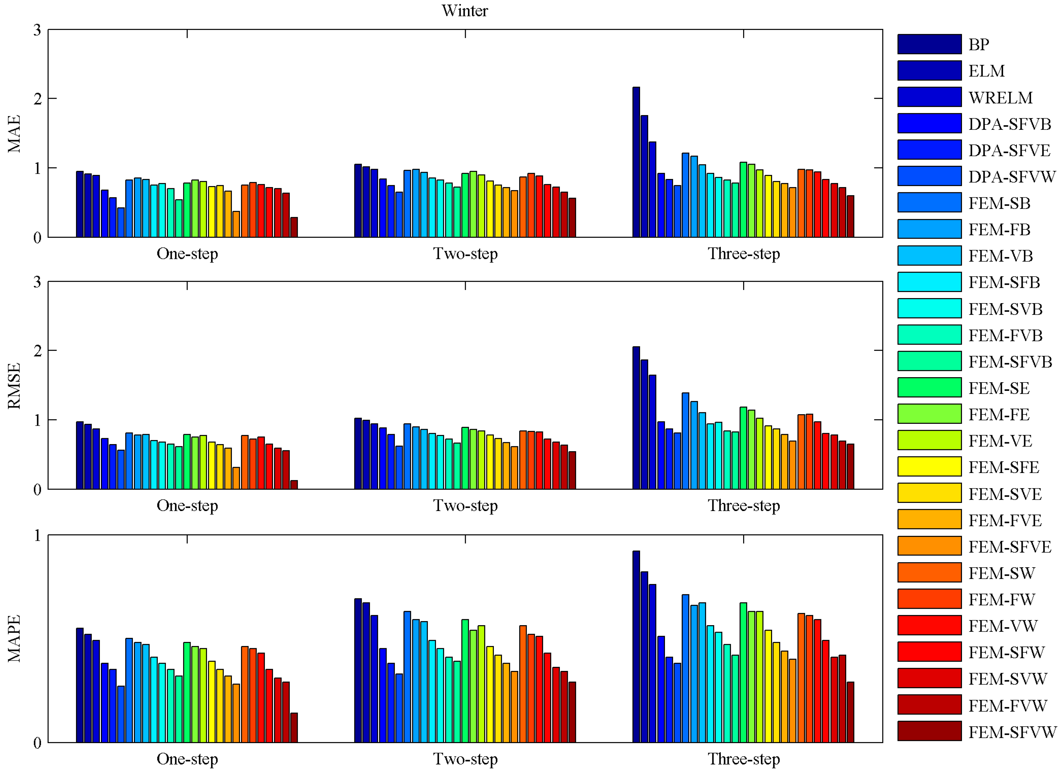
| Single | BP | 0.95 | 0.97 | 0.55 | 1.05 | 1.02 | 0.69 | 2.16 | 2.05 | 0.92 |
| ELM | 0.91 | 0.93 | 0.52 | 1.01 | 0.99 | 0.67 | 1.75 | 1.86 | 0.82 | |
| WRELM | 0.89 | 0.87 | 0.49 | 0.98 | 0.94 | 0.61 | 1.37 | 1.64 | 0.76 | |
| DPA | DPA-SFVB | 0.68 | 0.73 | 0.38 | 0.84 | 0.88 | 0.45 | 0.92 | 0.97 | 0.51 |
| DPA-SFVE | 0.57 | 0.64 | 0.35 | 0.74 | 0.79 | 0.38 | 0.83 | 0.87 | 0.41 | |
| DPA-SFVW | 0.42 | 0.56 | 0.27 | 0.65 | 0.62 | 0.33 | 0.74 | 0.81 | 0.38 | |
| FEM | FEM-SB | 0.82 | 0.81 | 0.50 | 0.96 | 0.94 | 0.63 | 1.21 | 1.39 | 0.71 |
| FEM-FB | 0.85 | 0.78 | 0.48 | 0.98 | 0.90 | 0.59 | 1.17 | 1.26 | 0.66 | |
| FEM-VB | 0.83 | 0.79 | 0.47 | 0.93 | 0.86 | 0.58 | 1.04 | 1.10 | 0.67 | |
| FEM-SFB | 0.75 | 0.70 | 0.41 | 0.85 | 0.80 | 0.49 | 0.92 | 0.94 | 0.56 | |
| FEM-SVB | 0.77 | 0.68 | 0.38 | 0.82 | 0.77 | 0.45 | 0.86 | 0.96 | 0.53 | |
| FEM-FVB | 0.70 | 0.65 | 0.35 | 0.78 | 0.72 | 0.41 | 0.82 | 0.84 | 0.47 | |
| FEM-SFVB | 0.54 | 0.61 | 0.32 | 0.72 | 0.66 | 0.39 | 0.78 | 0.82 | 0.42 | |
| FEM-SE | 0.78 | 0.79 | 0.48 | 0.92 | 0.89 | 0.59 | 1.08 | 1.18 | 0.67 | |
| FEM-FE | 0.82 | 0.75 | 0.46 | 0.95 | 0.86 | 0.54 | 1.05 | 1.14 | 0.63 | |
| FEM-VE | 0.80 | 0.77 | 0.45 | 0.90 | 0.84 | 0.56 | 0.97 | 1.02 | 0.63 | |
| FEM-SFE | 0.73 | 0.68 | 0.39 | 0.81 | 0.78 | 0.46 | 0.89 | 0.91 | 0.54 | |
| FEM-SVE | 0.74 | 0.64 | 0.35 | 0.75 | 0.73 | 0.42 | 0.80 | 0.87 | 0.48 | |
| FEM-FVE | 0.66 | 0.59 | 0.32 | 0.71 | 0.67 | 0.38 | 0.77 | 0.79 | 0.44 | |
| FEM-SFVE | 0.37 | 0.31 | 0.28 | 0.67 | 0.61 | 0.34 | 0.71 | 0.69 | 0.40 | |
| FEM-SW | 0.75 | 0.77 | 0.46 | 0.87 | 0.84 | 0.56 | 0.98 | 1.07 | 0.62 | |
| FEM-FW | 0.79 | 0.72 | 0.45 | 0.92 | 0.83 | 0.52 | 0.97 | 1.08 | 0.61 | |
| FEM-VW | 0.76 | 0.75 | 0.43 | 0.88 | 0.82 | 0.51 | 0.94 | 0.97 | 0.59 | |
| FEM-SFW | 0.71 | 0.65 | 0.35 | 0.76 | 0.72 | 0.43 | 0.83 | 0.80 | 0.49 | |
| FEM-SVW | 0.70 | 0.59 | 0.31 | 0.72 | 0.68 | 0.36 | 0.77 | 0.78 | 0.41 | |
| FEM-FVW | 0.63 | 0.55 | 0.29 | 0.65 | 0.63 | 0.34 | 0.71 | 0.69 | 0.42 | |
| FEM-SFVW | 0.28 | 0.12 | 0.14 | 0.56 | 0.54 | 0.29 | 0.60 | 0.65 | 0.29 | |
| Cases | Prediction Horizon | Errors | The Proportion of Reduction | |||||
|---|---|---|---|---|---|---|---|---|
| FEM-SFVB vs. DPA-SFVB | FEM-SFVE vs. DPA-SFVE | FEM-SFVW vs. DPA-SFVW | WRELM vs. BP | WRELM vs. ELM | ELM vs. BP | |||
| Spring | One-step ahead | MAE (%) | 23.38 | 25.00 | 49.21 | 2.88 | 0.98 | 1.92 |
| RMSE (%) | 36.59 | 28.99 | 58.33 | 14.35 | 4.02 | 10.76 | ||
| MAPE (%) | 19.35 | 24.14 | 50.00 | 9.76 | 5.13 | 4.88 | ||
| Two-step ahead | MAE (%) | 23.60 | 21.79 | 39.44 | 9.52 | 6.56 | 3.17 | |
| RMSE (%) | 18.28 | 28.40 | 43.10 | 10.79 | 4.98 | 6.12 | ||
| MAPE (%) | 18.42 | 15.63 | 48.00 | 9.26 | 5.77 | 3.70 | ||
| Three-step ahead | MAE (%) | 24.47 | 24.42 | 35.06 | 8.67 | 3.07 | 5.78 | |
| RMSE (%) | 14.14 | 21.98 | 25.64 | 13.65 | 10.28 | 3.75 | ||
| MAPE (%) | 21.15 | 14.29 | 51.72 | 7.35 | 3.08 | 4.41 | ||
| Summer | One-step ahead | MAE (%) | 14.63 | 16.46 | 50.00 | 9.57 | 4.49 | 5.32 |
| RMSE (%) | 17.89 | 18.68 | 70.69 | 11.61 | 8.33 | 3.57 | ||
| MAPE (%) | 11.11 | 23.26 | 34.48 | 20.55 | 15.94 | 5.48 | ||
| Two-step ahead | MAE (%) | 8.24 | 12.20 | 18.99 | 15.32 | 11.02 | 4.84 | |
| RMSE (%) | 9.09 | 13.68 | 22.47 | 23.46 | 16.46 | 8.38 | ||
| MAPE (%) | 13.21 | 10.20 | 10.64 | 17.44 | 8.97 | 9.30 | ||
| Three-step ahead | MAE (%) | 6.12 | 12.79 | 18.07 | 24.58 | 11.18 | 15.08 | |
| RMSE (%) | 15.18 | 12.37 | 12.77 | 32.00 | 14.22 | 20.73 | ||
| MAPE (%) | 18.46 | 17.74 | 12.50 | 16.50 | 5.49 | 11.65 | ||
| Fall | One-step ahead | MAE (%) | 20.83 | 35.38 | 67.92 | 7.84 | 3.09 | 4.90 |
| RMSE (%) | 24.64 | 25.53 | 89.58 | 10.10 | 6.32 | 4.04 | ||
| MAPE (%) | 28.89 | 19.44 | 21.74 | 9.68 | 5.08 | 4.84 | ||
| Two-step ahead | MAE (%) | 16.47 | 18.06 | 41.94 | 20.31 | 12.07 | 9.38 | |
| RMSE (%) | 23.60 | 18.42 | 67.16 | 13.21 | 9.80 | 3.77 | ||
| MAPE (%) | 12.77 | 11.36 | 21.43 | 10.81 | 4.35 | 6.76 | ||
| Three-step ahead | MAE (%) | 12.64 | 21.79 | 46.27 | 19.49 | 9.77 | 10.77 | |
| RMSE (%) | 15.05 | 15.29 | 67.12 | 25.53 | 11.02 | 16.31 | ||
| MAPE (%) | 9.09 | 11.76 | 27.08 | 10.20 | 4.35 | 6.12 | ||
| Winter | One-step ahead | MAE (%) | 20.59 | 35.09 | 33.33 | 6.32 | 2.20 | 4.21 |
| RMSE (%) | 16.44 | 51.56 | 78.57 | 10.31 | 6.45 | 4.12 | ||
| MAPE (%) | 15.79 | 20.00 | 48.15 | 10.91 | 5.77 | 5.45 | ||
| Two-step ahead | MAE (%) | 14.29 | 9.46 | 13.85 | 6.67 | 2.97 | 3.81 | |
| RMSE (%) | 25.00 | 22.78 | 12.90 | 7.84 | 5.05 | 2.94 | ||
| MAPE (%) | 13.33 | 10.53 | 12.12 | 11.59 | 8.96 | 2.90 | ||
| Three-step ahead | MAE (%) | 15.22 | 14.46 | 18.92 | 36.57 | 21.71 | 18.98 | |
| RMSE (%) | 15.46 | 20.69 | 19.75 | 20.00 | 11.83 | 9.27 | ||
| MAPE (%) | 17.65 | 2.44 | 23.68 | 17.39 | 7.32 | 10.87 | ||
| Comparison of Models | Spring | ||||||||
|---|---|---|---|---|---|---|---|---|---|
| One-Step Ahead | Two-Step Ahead | Three-Step Ahead | |||||||
| MAE (%) | RMSE (%) | MAPE (%) | MAE (%) | RMSE (%) | MAPE (%) | MAE (%) | RMSE (%) | MAPE (%) | |
| FEM-SFVB vs. FEM-SFB | 25.32 | 52.29 | 13.79 | 20.00 | 38.71 | 24.39 | 28.28 | 37.04 | 24.07 |
| FEM-SFVB vs. FEM-SVB | 22.37 | 47.47 | 16.67 | 16.05 | 28.97 | 26.19 | 20.22 | 27.97 | 22.64 |
| FEM-SFVB vs. FEM-FVB | 16.90 | 37.35 | 7.41 | 6.85 | 12.64 | 20.51 | 10.13 | 7.61 | 19.61 |
| FEM-SFVE vs. FEM-SFE | 28.00 | 52.43 | 21.43 | 22.78 | 51.26 | 32.50 | 30.85 | 42.28 | 32.08 |
| FEM-SFVE vs. FEM-SVE | 25.00 | 48.42 | 24.14 | 18.67 | 43.69 | 34.15 | 22.62 | 34.86 | 30.77 |
| FEM-SFVE vs. FEM-FVE | 19.40 | 37.18 | 12.00 | 12.86 | 28.40 | 25.00 | 9.72 | 19.32 | 26.53 |
| FEM-SFVW vs. FEM-SFW | 54.93 | 79.38 | 62.96 | 44.16 | 69.44 | 66.67 | 43.82 | 50.43 | 73.08 |
| FEM-SFVW vs. FEM-SVW | 52.94 | 77.53 | 64.29 | 41.10 | 65.63 | 66.67 | 36.71 | 42.57 | 72.55 |
| FEM-SFVW vs. FEM-FVW | 41.82 | 65.52 | 52.38 | 31.75 | 52.17 | 60.61 | 26.47 | 20.55 | 71.43 |
| FEM-SFB vs. FEM-SB | 16.84 | 40.11 | 17.14 | 19.81 | 42.06 | 14.58 | 32.65 | 48.28 | 11.48 |
| FEM-SFB vs. FEM-FB | 11.24 | 37.36 | 23.68 | 13.27 | 37.06 | 18.00 | 20.80 | 33.50 | 12.90 |
| FEM-SVB vs. FEM-SB | 20.00 | 45.60 | 14.29 | 23.58 | 50.00 | 12.50 | 39.46 | 54.79 | 13.11 |
| FEM-SVB vs. FEM-VB | 18.28 | 41.42 | 16.67 | 18.18 | 42.16 | 12.50 | 32.58 | 39.80 | 11.67 |
| FEM-FVB vs. FEM-FB | 20.22 | 52.30 | 28.95 | 25.51 | 55.84 | 22.00 | 36.80 | 54.68 | 17.74 |
| FEM-FVB vs. FEM-VB | 23.66 | 50.89 | 25.00 | 26.26 | 52.97 | 18.75 | 40.15 | 53.06 | 15.00 |
| FEM-SFE vs. FEM-SE | 17.58 | 34.39 | 15.15 | 21.78 | 39.90 | 16.67 | 32.37 | 40.58 | 11.67 |
| FEM-SFE vs. FEM-FE | 13.79 | 28.97 | 24.32 | 17.71 | 33.52 | 14.89 | 22.31 | 34.57 | 10.17 |
| FEM-SVE vs. FEM-SE | 20.88 | 39.49 | 12.12 | 25.74 | 47.98 | 14.58 | 39.57 | 47.34 | 13.33 |
| FEM-SVE vs. FEM-VE | 19.10 | 37.09 | 17.14 | 22.68 | 43.41 | 8.89 | 26.32 | 42.93 | 8.77 |
| FEM-FVE vs. FEM-FE | 22.99 | 46.21 | 32.43 | 27.08 | 54.75 | 23.40 | 40.50 | 53.19 | 16.95 |
| FEM-FVE vs. FEM-VE | 24.72 | 48.34 | 28.57 | 27.84 | 55.49 | 20.00 | 36.84 | 53.93 | 14.04 |
| FEM-SFW vs. FEM-SW | 13.41 | 21.14 | 6.90 | 18.09 | 40.66 | 15.22 | 27.64 | 40.31 | 10.34 |
| FEM-SFW vs. FEM-FW | 11.25 | 16.38 | 18.18 | 15.38 | 35.71 | 11.36 | 24.58 | 33.90 | 8.77 |
| FEM-SVW vs. FEM-SW | 17.07 | 27.64 | 3.45 | 22.34 | 47.25 | 15.22 | 35.77 | 48.47 | 12.07 |
| FEM-SVW vs. FEM-VW | 16.05 | 26.45 | 9.68 | 17.05 | 37.66 | 13.33 | 22.55 | 38.04 | 8.93 |
| FEM-FVW vs. FEM-FW | 31.25 | 50.00 | 36.36 | 30.77 | 58.93 | 25.00 | 42.37 | 58.76 | 14.04 |
| FEM-FVW vs. FEM-VW | 32.10 | 52.07 | 32.26 | 28.41 | 55.19 | 26.67 | 33.33 | 55.21 | 12.50 |
| FEM-SB vs. BP | 8.65 | 18.39 | 14.63 | 15.87 | 23.02 | 11.11 | 15.03 | 10.92 | 10.29 |
| FEM-FB vs. BP | 14.42 | 21.97 | 7.32 | 22.22 | 29.14 | 7.41 | 27.75 | 30.72 | 8.82 |
| FEM-VB vs. BP | 10.58 | 24.22 | 12.20 | 21.43 | 33.45 | 11.11 | 23.70 | 33.11 | 11.76 |
| FEM-SE vs. ELM | 10.78 | 21.11 | 15.38 | 17.21 | 24.14 | 7.69 | 14.72 | 26.60 | 7.69 |
| FEM-FE vs. ELM | 14.71 | 27.14 | 5.13 | 21.31 | 31.42 | 9.62 | 25.77 | 33.33 | 9.23 |
| FEM-VE vs. ELM | 12.75 | 24.12 | 10.26 | 20.49 | 30.27 | 13.46 | 30.06 | 32.27 | 12.31 |
| FEM-SW vs. WRELM | 18.81 | 35.60 | 21.62 | 17.54 | 26.61 | 6.12 | 22.15 | 22.53 | 7.94 |
| FEM-FW vs. WRELM | 20.79 | 39.27 | 10.81 | 20.18 | 32.26 | 10.20 | 25.32 | 30.04 | 9.52 |
| FEM-VW vs. WRELM | 19.80 | 36.65 | 16.22 | 22.81 | 37.90 | 8.16 | 35.44 | 35.57 | 11.11 |
| Comparison of Models | Summer | ||||||||
|---|---|---|---|---|---|---|---|---|---|
| One-Step Ahead | Two-Step Ahead | Three-Step Ahead | |||||||
| MAE (%) | RMSE (%) | MAPE (%) | MAE (%) | RMSE (%) | MAPE (%) | MAE (%) | RMSE (%) | MAPE (%) | |
| FEM-SFVB vs. FEM-SFB | 5.41 | 12.36 | 18.37 | 4.88 | 5.26 | 9.80 | 10.68 | 15.93 | 10.17 |
| FEM-SFVB vs. FEM-SVB | 10.26 | 12.36 | 20.00 | 8.24 | 6.25 | 13.21 | 15.60 | 8.65 | 3.64 |
| FEM-SFVB vs. FEM-FVB | 7.89 | 14.29 | 11.11 | 3.70 | 5.26 | 4.17 | 7.07 | 1.04 | 5.36 |
| FEM-SFVE vs. FEM-SFE | 7.04 | 6.33 | 26.67 | 10.00 | 5.75 | 6.38 | 24.24 | 16.67 | 7.27 |
| FEM-SFVE vs. FEM-SVE | 13.16 | 8.64 | 29.79 | 12.20 | 2.38 | 10.20 | 19.35 | 13.27 | 8.93 |
| FEM-SFVE vs. FEM-FVE | 7.04 | 9.76 | 15.38 | 7.69 | 3.53 | 2.22 | 7.41 | 4.49 | 3.77 |
| FEM-SFVW vs. FEM-SFW | 52.94 | 77.92 | 55.81 | 17.95 | 15.85 | 8.70 | 27.66 | 14.58 | 3.92 |
| FEM-SFVW vs. FEM-SVW | 55.56 | 75.71 | 57.78 | 16.88 | 12.66 | 10.64 | 21.84 | 12.77 | 5.77 |
| FEM-SFVW vs. FEM-FVW | 52.94 | 77.33 | 47.22 | 9.86 | 13.75 | 4.55 | 10.53 | 2.38 | 2.00 |
| FEM-SFB vs. FEM-SB | 13.95 | 6.32 | 19.67 | 28.70 | 26.36 | 32.00 | 33.55 | 34.68 | 33.71 |
| FEM-SFB vs. FEM-FB | 11.90 | 8.25 | 14.04 | 24.77 | 29.10 | 20.31 | 27.97 | 37.57 | 24.36 |
| FEM-SVB vs. FEM-SB | 9.30 | 6.32 | 18.03 | 26.09 | 25.58 | 29.33 | 29.68 | 39.88 | 38.20 |
| FEM-SVB vs. FEM-VB | 8.24 | 5.32 | 9.09 | 12.37 | 26.72 | 19.70 | 14.17 | 39.18 | 20.29 |
| FEM-FVB vs. FEM-FB | 9.52 | 6.19 | 21.05 | 25.69 | 29.10 | 25.00 | 30.77 | 46.96 | 28.21 |
| FEM-FVB vs. FEM-VB | 10.59 | 3.19 | 18.18 | 16.49 | 27.48 | 27.27 | 22.05 | 43.86 | 18.84 |
| FEM-SFE vs. FEM-SE | 14.46 | 11.24 | 21.05 | 25.23 | 25.00 | 30.88 | 29.79 | 35.44 | 28.57 |
| FEM-SFE vs. FEM-FE | 11.25 | 15.96 | 11.76 | 19.19 | 31.50 | 22.95 | 27.21 | 31.08 | 20.29 |
| FEM-SVE vs. FEM-SE | 8.43 | 8.99 | 17.54 | 23.36 | 27.59 | 27.94 | 34.04 | 37.97 | 27.27 |
| FEM-SVE vs. FEM-VE | 3.80 | 8.99 | 11.32 | 12.77 | 34.88 | 20.97 | 19.83 | 28.47 | 13.85 |
| FEM-FVE vs. FEM-FE | 11.25 | 12.77 | 23.53 | 21.21 | 33.07 | 26.23 | 40.44 | 39.86 | 23.19 |
| FEM-FVE vs. FEM-VE | 10.13 | 7.87 | 26.42 | 17.02 | 34.11 | 27.42 | 30.17 | 35.04 | 18.46 |
| FEM-SFW vs. FEM-SW | 16.05 | 9.41 | 21.82 | 20.41 | 19.61 | 26.98 | 25.98 | 35.57 | 28.17 |
| FEM-SFW vs. FEM-FW | 12.82 | 15.38 | 12.24 | 17.89 | 30.51 | 20.69 | 25.40 | 27.27 | 21.54 |
| FEM-SVW vs. FEM-SW | 11.11 | 17.65 | 18.18 | 21.43 | 22.55 | 25.40 | 31.50 | 36.91 | 26.76 |
| FEM-SVW vs. FEM-VW | 4.00 | 20.45 | 11.76 | 13.48 | 26.85 | 16.07 | 20.18 | 22.31 | 17.46 |
| FEM-FVW vs. FEM-FW | 12.82 | 17.58 | 26.53 | 25.26 | 32.20 | 24.14 | 39.68 | 36.36 | 23.08 |
| FEM-FVW vs. FEM-VW | 9.33 | 14.77 | 29.41 | 20.22 | 25.93 | 21.43 | 30.28 | 30.58 | 20.63 |
| FEM-SB vs. BP | 8.51 | 15.18 | 16.44 | 7.26 | 27.93 | 12.79 | 13.41 | 37.09 | 13.59 |
| FEM-FB vs. BP | 10.64 | 13.39 | 21.92 | 12.10 | 25.14 | 25.58 | 20.11 | 34.18 | 24.27 |
| FEM-VB vs. BP | 9.57 | 16.07 | 24.66 | 21.77 | 26.82 | 23.26 | 29.05 | 37.82 | 33.01 |
| FEM-SE vs. ELM | 6.74 | 17.59 | 17.39 | 9.32 | 29.27 | 12.82 | 7.24 | 27.52 | 15.38 |
| FEM-FE vs. ELM | 10.11 | 12.96 | 26.09 | 16.10 | 22.56 | 21.79 | 10.53 | 32.11 | 24.18 |
| FEM-VE vs. ELM | 11.24 | 17.59 | 23.19 | 20.34 | 21.34 | 20.51 | 23.68 | 37.16 | 28.57 |
| FEM-SW vs. WRELM | 4.71 | 14.14 | 5.17 | 6.67 | 25.55 | 11.27 | 5.93 | 20.32 | 17.44 |
| FEM-FW vs. WRELM | 8.24 | 8.08 | 15.52 | 9.52 | 13.87 | 18.31 | 6.67 | 29.41 | 24.42 |
| FEM-VW vs. WRELM | 11.76 | 11.11 | 12.07 | 15.24 | 21.17 | 21.13 | 19.26 | 35.29 | 26.74 |
| Comparison of Models | Fall | ||||||||
|---|---|---|---|---|---|---|---|---|---|
| One-Step Ahead | Two-Step Ahead | Three-Step Ahead | |||||||
| MAE (%) | RMSE (%) | MAPE (%) | MAE (%) | RMSE (%) | MAPE (%) | MAE (%) | RMSE (%) | MAPE (%) | |
| FEM-SFVB vs. FEM-SFB | 26.92 | 29.73 | 28.89 | 13.41 | 13.92 | 22.64 | 9.52 | 13.19 | 18.03 |
| FEM-SFVB vs. FEM-SVB | 28.75 | 30.67 | 23.81 | 15.48 | 16.05 | 18.00 | 11.63 | 9.20 | 13.79 |
| FEM-SFVB vs. FEM-FVB | 26.92 | 24.64 | 20.00 | 11.25 | 10.53 | 8.89 | 6.17 | 4.82 | 9.09 |
| FEM-SFVE vs. FEM-SFE | 44.00 | 50.00 | 32.56 | 24.36 | 18.42 | 22.00 | 24.69 | 15.29 | 22.41 |
| FEM-SFVE vs. FEM-SVE | 46.15 | 52.05 | 29.27 | 27.16 | 20.51 | 17.02 | 24.69 | 13.25 | 15.09 |
| FEM-SFVE vs. FEM-FVE | 41.67 | 48.53 | 19.44 | 24.36 | 15.07 | 7.14 | 22.78 | 7.69 | 11.76 |
| FEM-SFVW vs. FEM-SFW | 76.39 | 92.75 | 56.10 | 51.35 | 69.01 | 29.79 | 53.25 | 70.37 | 38.60 |
| FEM-SFVW vs. FEM-SVW | 76.06 | 92.65 | 51.35 | 52.00 | 69.44 | 21.43 | 54.43 | 69.62 | 31.37 |
| FEM-SFVW vs. FEM-FVW | 74.24 | 92.06 | 43.75 | 49.30 | 67.65 | 10.81 | 51.35 | 66.67 | 22.22 |
| FEM-SFB vs. FEM-SB | 17.89 | 19.57 | 18.18 | 24.07 | 17.71 | 20.90 | 46.84 | 24.79 | 26.51 |
| FEM-SFB vs. FEM-FB | 15.22 | 16.85 | 15.09 | 15.46 | 14.13 | 17.19 | 34.88 | 19.47 | 19.74 |
| FEM-SVB vs. FEM-SB | 15.79 | 18.48 | 23.64 | 22.22 | 15.63 | 25.37 | 45.57 | 28.10 | 30.12 |
| FEM-SVB vs. FEM-VB | 9.09 | 19.35 | 19.23 | 8.70 | 17.35 | 18.03 | 11.34 | 17.14 | 20.55 |
| FEM-FVB vs. FEM-FB | 15.22 | 22.47 | 24.53 | 17.53 | 17.39 | 29.69 | 37.21 | 26.55 | 27.63 |
| FEM-FVB vs. FEM-VB | 11.36 | 25.81 | 23.08 | 13.04 | 22.45 | 26.23 | 16.49 | 20.95 | 24.66 |
| FEM-SFE vs. FEM-SE | 17.58 | 20.45 | 18.87 | 21.21 | 15.56 | 23.08 | 40.88 | 16.67 | 26.58 |
| FEM-SFE vs. FEM-FE | 15.73 | 16.67 | 14.00 | 17.02 | 11.63 | 18.03 | 30.17 | 19.05 | 18.31 |
| FEM-SVE vs. FEM-SE | 14.29 | 17.05 | 22.64 | 18.18 | 13.33 | 27.69 | 40.88 | 18.63 | 32.91 |
| FEM-SVE vs. FEM-VE | 8.24 | 16.09 | 16.33 | 7.95 | 17.89 | 17.54 | 11.96 | 14.43 | 19.70 |
| FEM-FVE vs. FEM-FE | 19.10 | 19.05 | 28.00 | 17.02 | 15.12 | 31.15 | 31.90 | 25.71 | 28.17 |
| FEM-FVE vs. FEM-VE | 15.29 | 21.84 | 26.53 | 11.36 | 23.16 | 26.32 | 14.13 | 19.59 | 22.73 |
| FEM-SFW vs. FEM-SW | 19.10 | 18.82 | 16.33 | 22.92 | 20.22 | 25.40 | 38.89 | 14.74 | 24.00 |
| FEM-SFW vs. FEM-FW | 16.28 | 12.66 | 12.77 | 18.68 | 13.41 | 18.97 | 23.76 | 16.49 | 14.93 |
| FEM-SVW vs. FEM-SW | 20.22 | 20.00 | 24.49 | 21.88 | 19.10 | 33.33 | 37.30 | 16.84 | 32.00 |
| FEM-SVW vs. FEM-VW | 14.46 | 19.05 | 22.92 | 11.76 | 20.88 | 23.64 | 11.24 | 15.05 | 19.05 |
| FEM-FVW vs. FEM-FW | 23.26 | 20.25 | 31.91 | 21.98 | 17.07 | 36.21 | 26.73 | 25.77 | 32.84 |
| FEM-FVW vs. FEM-VW | 20.48 | 25.00 | 33.33 | 16.47 | 25.27 | 32.73 | 16.85 | 22.58 | 28.57 |
| FEM-SB vs. BP | 6.86 | 7.07 | 11.29 | 15.63 | 9.43 | 9.46 | 18.97 | 14.18 | 15.31 |
| FEM-FB vs. BP | 9.80 | 10.10 | 14.52 | 24.22 | 13.21 | 13.51 | 33.85 | 19.86 | 22.45 |
| FEM-VB vs. BP | 13.73 | 6.06 | 16.13 | 28.13 | 7.55 | 17.57 | 50.26 | 25.53 | 25.51 |
| FEM-SE vs. ELM | 6.19 | 7.37 | 10.17 | 14.66 | 11.76 | 5.80 | 21.26 | 13.56 | 14.13 |
| FEM-FE vs. ELM | 8.25 | 11.58 | 15.25 | 18.97 | 15.69 | 11.59 | 33.33 | 11.02 | 22.83 |
| FEM-VE vs. ELM | 12.37 | 8.42 | 16.95 | 24.14 | 6.86 | 17.39 | 47.13 | 17.80 | 28.26 |
| FEM-SW vs. WRELM | 5.32 | 4.49 | 12.50 | 5.88 | 3.26 | 4.55 | 19.75 | 9.52 | 14.77 |
| FEM-FW vs. WRELM | 8.51 | 11.24 | 16.07 | 10.78 | 10.87 | 12.12 | 35.67 | 7.62 | 23.86 |
| FEM-VW vs. WRELM | 11.70 | 5.62 | 14.29 | 16.67 | 1.09 | 16.67 | 43.31 | 11.43 | 28.41 |
| Comparison of Models | Winter | ||||||||
|---|---|---|---|---|---|---|---|---|---|
| One-Step Ahead | Two-Step Ahead | Three-Step Ahead | |||||||
| MAE (%) | RMSE (%) | MAPE (%) | MAE (%) | RMSE (%) | MAPE (%) | MAE (%) | RMSE (%) | MAPE (%) | |
| FEM-SFVB vs. FEM-SFB | 28.00 | 12.86 | 21.95 | 15.29 | 17.50 | 20.41 | 15.22 | 12.77 | 25.00 |
| FEM-SFVB vs. FEM-SVB | 29.87 | 10.29 | 15.79 | 12.20 | 14.29 | 13.33 | 9.30 | 14.58 | 20.75 |
| FEM-SFVB vs. FEM-FVB | 22.86 | 6.15 | 8.57 | 7.69 | 8.33 | 4.88 | 4.88 | 2.38 | 10.64 |
| FEM-SFVE vs. FEM-SFE | 49.32 | 54.41 | 28.21 | 17.28 | 21.79 | 26.09 | 20.22 | 24.18 | 25.93 |
| FEM-SFVE vs. FEM-SVE | 50.00 | 51.56 | 20.00 | 10.67 | 16.44 | 19.05 | 11.25 | 20.69 | 16.67 |
| FEM-SFVE vs. FEM-FVE | 43.94 | 47.46 | 12.50 | 5.63 | 8.96 | 10.53 | 7.79 | 12.66 | 9.09 |
| FEM-SFVW vs. FEM-SFW | 60.56 | 81.54 | 60.00 | 26.32 | 25.00 | 32.56 | 27.71 | 18.75 | 40.82 |
| FEM-SFVW vs. FEM-SVW | 60.00 | 79.66 | 54.84 | 22.22 | 20.59 | 19.44 | 22.08 | 16.67 | 29.27 |
| FEM-SFVW vs. FEM-FVW | 55.56 | 78.18 | 51.72 | 13.85 | 14.29 | 14.71 | 15.49 | 5.80 | 30.95 |
| FEM-SFB vs. FEM-SB | 8.54 | 13.58 | 18.00 | 11.46 | 14.89 | 22.22 | 23.97 | 32.37 | 21.13 |
| FEM-SFB vs. FEM-FB | 11.76 | 10.26 | 14.58 | 13.27 | 11.11 | 16.95 | 21.37 | 25.40 | 15.15 |
| FEM-SVB vs. FEM-SB | 6.10 | 16.05 | 24.00 | 14.58 | 18.09 | 28.57 | 28.93 | 30.94 | 25.35 |
| FEM-SVB vs. FEM-VB | 7.23 | 13.92 | 19.15 | 11.83 | 10.47 | 22.41 | 17.31 | 12.73 | 20.90 |
| FEM-FVB vs. FEM-FB | 17.65 | 16.67 | 27.08 | 20.41 | 20.00 | 30.51 | 29.91 | 33.33 | 28.79 |
| FEM-FVB vs. FEM-VB | 15.66 | 17.72 | 25.53 | 16.13 | 16.28 | 29.31 | 21.15 | 23.64 | 29.85 |
| FEM-SFE vs. FEM-SE | 6.41 | 13.92 | 18.75 | 11.96 | 12.36 | 22.03 | 17.59 | 22.88 | 19.40 |
| FEM-SFE vs. FEM-FE | 10.98 | 9.33 | 15.22 | 14.74 | 9.30 | 14.81 | 15.24 | 20.18 | 14.29 |
| FEM-SVE vs. FEM-SE | 5.13 | 18.99 | 27.08 | 18.48 | 17.98 | 28.81 | 25.93 | 26.27 | 28.36 |
| FEM-SVE vs. FEM-VE | 7.50 | 16.88 | 22.22 | 16.67 | 13.10 | 25.00 | 17.53 | 14.71 | 23.81 |
| FEM-FVE vs. FEM-FE | 19.51 | 21.33 | 30.43 | 25.26 | 22.09 | 29.63 | 26.67 | 30.70 | 30.16 |
| FEM-FVE vs. FEM-VE | 17.50 | 23.38 | 28.89 | 21.11 | 20.24 | 32.14 | 20.62 | 22.55 | 30.16 |
| FEM-SFW vs. FEM-SW | 5.33 | 15.58 | 23.91 | 12.64 | 14.29 | 23.21 | 15.31 | 25.23 | 20.97 |
| FEM-SFW vs. FEM-FW | 10.13 | 9.72 | 22.22 | 17.39 | 13.25 | 17.31 | 14.43 | 25.93 | 19.67 |
| FEM-SVW vs. FEM-SW | 6.67 | 23.38 | 32.61 | 17.24 | 19.05 | 35.71 | 21.43 | 27.10 | 33.87 |
| FEM-SVW vs. FEM-VW | 7.89 | 21.33 | 27.91 | 18.18 | 17.07 | 29.41 | 18.09 | 19.59 | 30.51 |
| FEM-FVW vs. FEM-FW | 20.25 | 23.61 | 35.56 | 29.35 | 24.10 | 34.62 | 26.80 | 36.11 | 31.15 |
| FEM-FVW vs. FEM-VW | 17.11 | 26.67 | 32.56 | 26.14 | 23.17 | 33.33 | 24.47 | 28.87 | 28.81 |
| FEM-SB vs. BP | 13.68 | 16.49 | 9.09 | 8.57 | 7.84 | 8.70 | 43.98 | 32.20 | 22.83 |
| FEM-FB vs. BP | 10.53 | 19.59 | 12.73 | 6.67 | 11.76 | 14.49 | 45.83 | 38.54 | 28.26 |
| FEM-VB vs. BP | 12.63 | 18.56 | 14.55 | 11.43 | 15.69 | 15.94 | 51.85 | 46.34 | 27.17 |
| FEM-SE vs. ELM | 14.29 | 15.05 | 7.69 | 8.91 | 10.10 | 11.94 | 38.29 | 36.56 | 18.29 |
| FEM-FE vs. ELM | 9.89 | 19.35 | 11.54 | 5.94 | 13.13 | 19.40 | 40.00 | 38.71 | 23.17 |
| FEM-VE vs. ELM | 12.09 | 17.20 | 13.46 | 10.89 | 15.15 | 16.42 | 44.57 | 45.16 | 23.17 |
| FEM-SW vs. WRELM | 15.73 | 11.49 | 6.12 | 11.22 | 10.64 | 8.20 | 28.47 | 34.76 | 18.42 |
| FEM-FW vs. WRELM | 11.24 | 17.24 | 8.16 | 6.12 | 11.70 | 14.75 | 29.20 | 34.15 | 19.74 |
| FEM-VW vs. WRELM | 14.61 | 13.79 | 12.24 | 10.20 | 12.77 | 16.39 | 31.39 | 40.85 | 22.37 |
© 2018 by the authors. Licensee MDPI, Basel, Switzerland. This article is an open access article distributed under the terms and conditions of the Creative Commons Attribution (CC BY) license (http://creativecommons.org/licenses/by/4.0/).
Share and Cite
Wang, J.; Wang, Y.; Li, Y. A Novel Hybrid Strategy Using Three-Phase Feature Extraction and a Weighted Regularized Extreme Learning Machine for Multi-Step Ahead Wind Speed Prediction. Energies 2018, 11, 321. https://doi.org/10.3390/en11020321
Wang J, Wang Y, Li Y. A Novel Hybrid Strategy Using Three-Phase Feature Extraction and a Weighted Regularized Extreme Learning Machine for Multi-Step Ahead Wind Speed Prediction. Energies. 2018; 11(2):321. https://doi.org/10.3390/en11020321
Chicago/Turabian StyleWang, Jujie, Yanfeng Wang, and Yaning Li. 2018. "A Novel Hybrid Strategy Using Three-Phase Feature Extraction and a Weighted Regularized Extreme Learning Machine for Multi-Step Ahead Wind Speed Prediction" Energies 11, no. 2: 321. https://doi.org/10.3390/en11020321
APA StyleWang, J., Wang, Y., & Li, Y. (2018). A Novel Hybrid Strategy Using Three-Phase Feature Extraction and a Weighted Regularized Extreme Learning Machine for Multi-Step Ahead Wind Speed Prediction. Energies, 11(2), 321. https://doi.org/10.3390/en11020321


