Efficient Power Scheduling in Smart Homes Using Hybrid Grey Wolf Differential Evolution Optimization Technique with Real Time and Critical Peak Pricing Schemes


 , , , , and
Abstract
:1. Introduction
2. Related Work
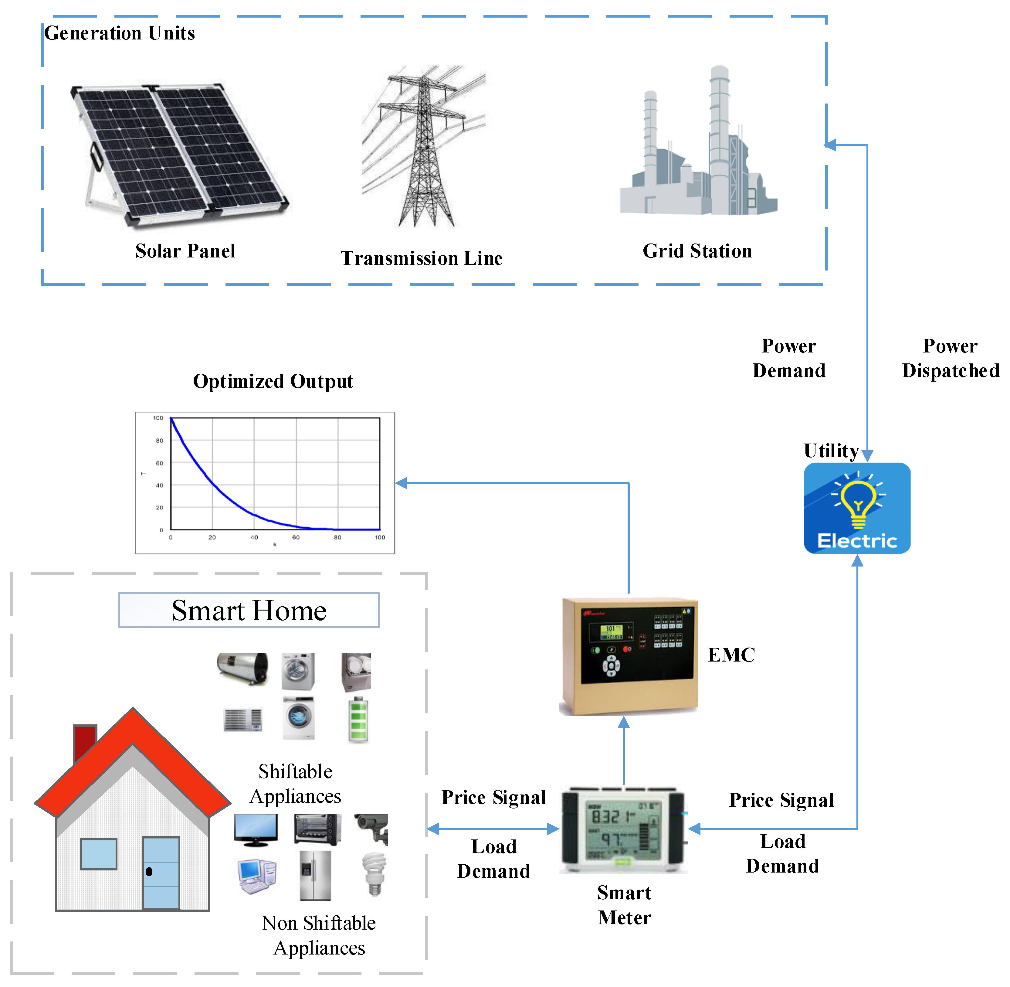
3. System Model
3.1. Classification of Appliances
3.1.1. Shiftable Appliances
3.1.2. Controllable Appliances
3.1.3. Non-Shiftable Appliances
4. Proposed Scheme
4.1. EDE
| Algorithm 1: EDE. |
 |
4.2. GWO
4.2.1. Encircling Prey
4.2.2. Hunting
| Algorithm 2: GWO. |
 |
4.3. HGWDE
| Algorithm 3: HGWDE. |
 |
5. Simulation and Results
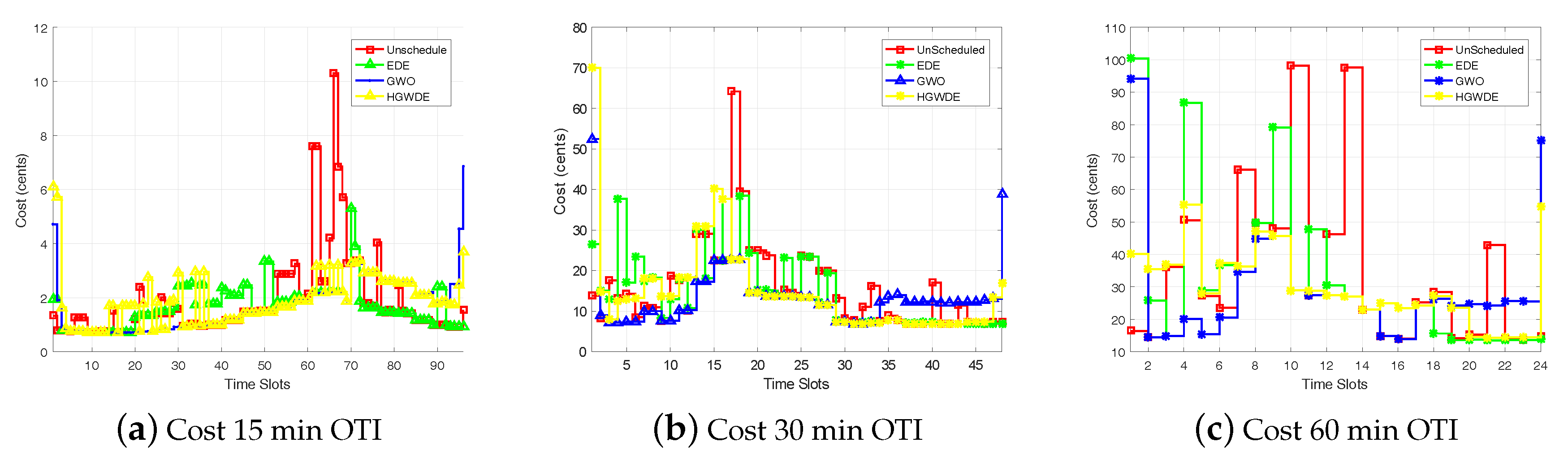
5.1. Cost
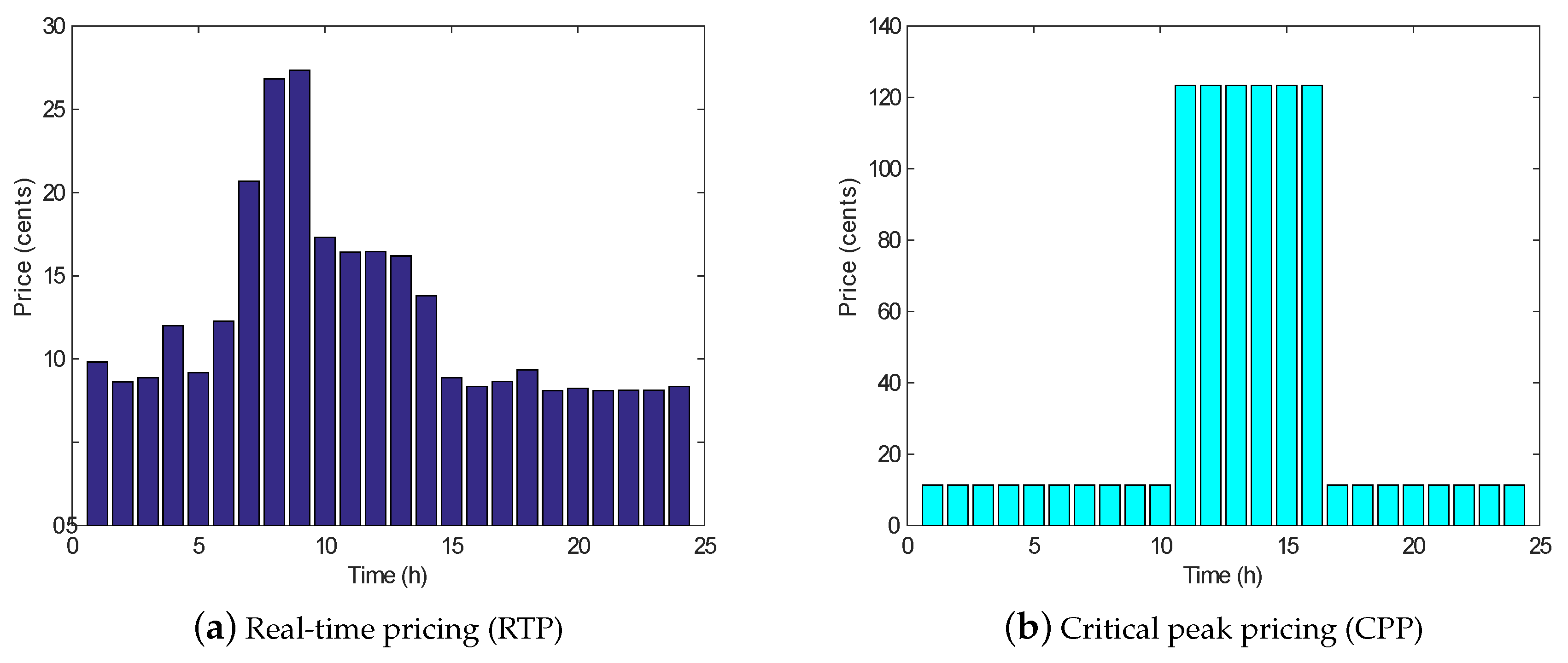
5.1.1. Cost Using RTP
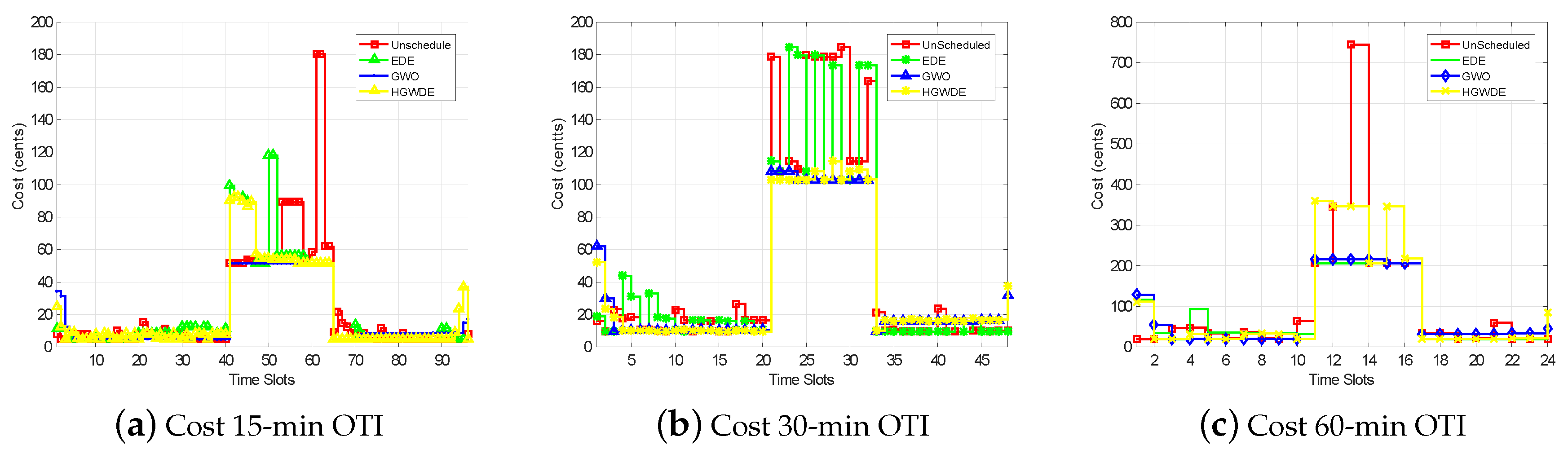
5.1.2. Cost using CPP
5.2. Energy Consumption
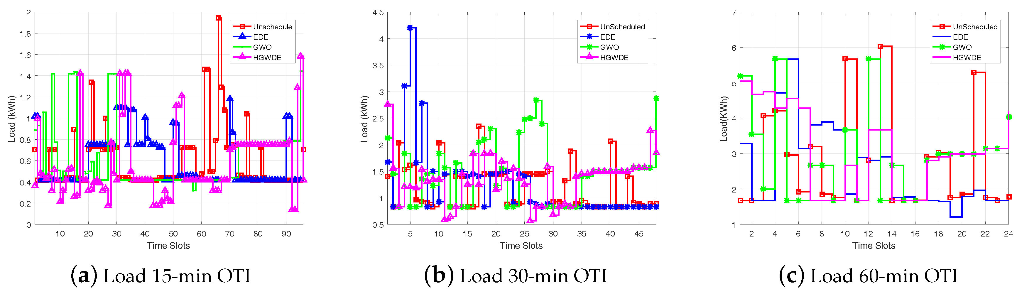
5.2.1. Load Using RTP
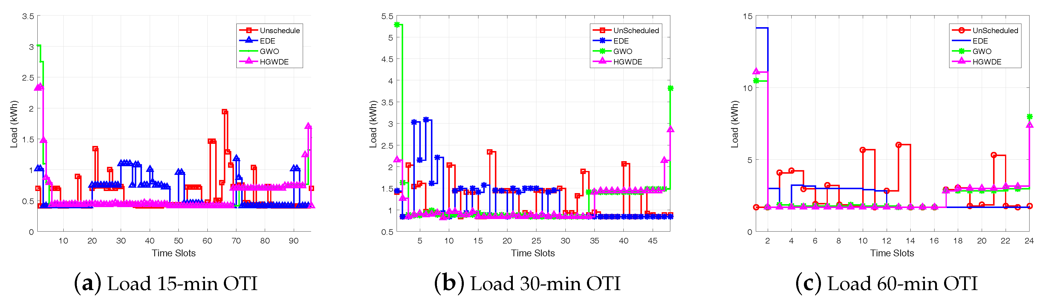
5.2.2. Load Using CPP
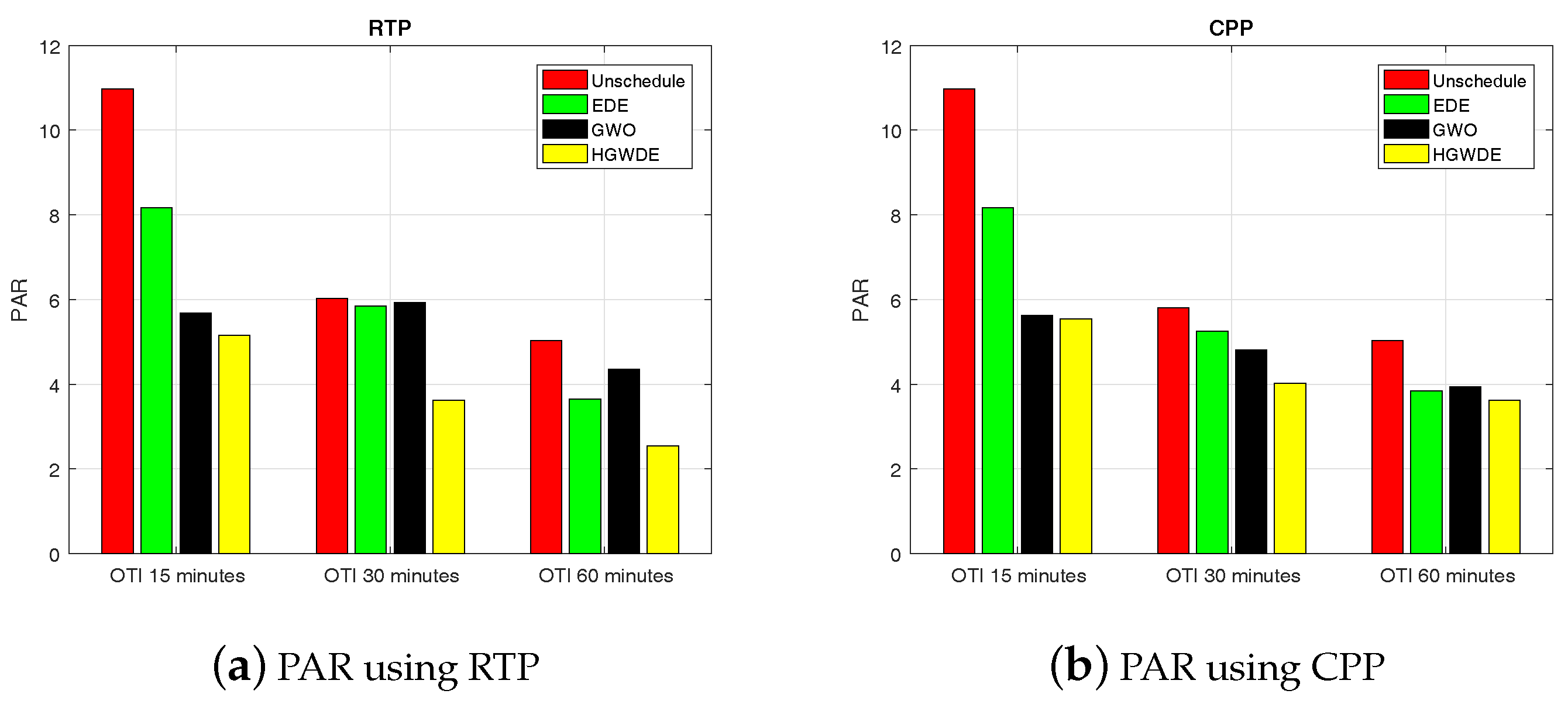
5.3. PAR
5.3.1. PAR Using RTP
5.3.2. PAR Using CPP
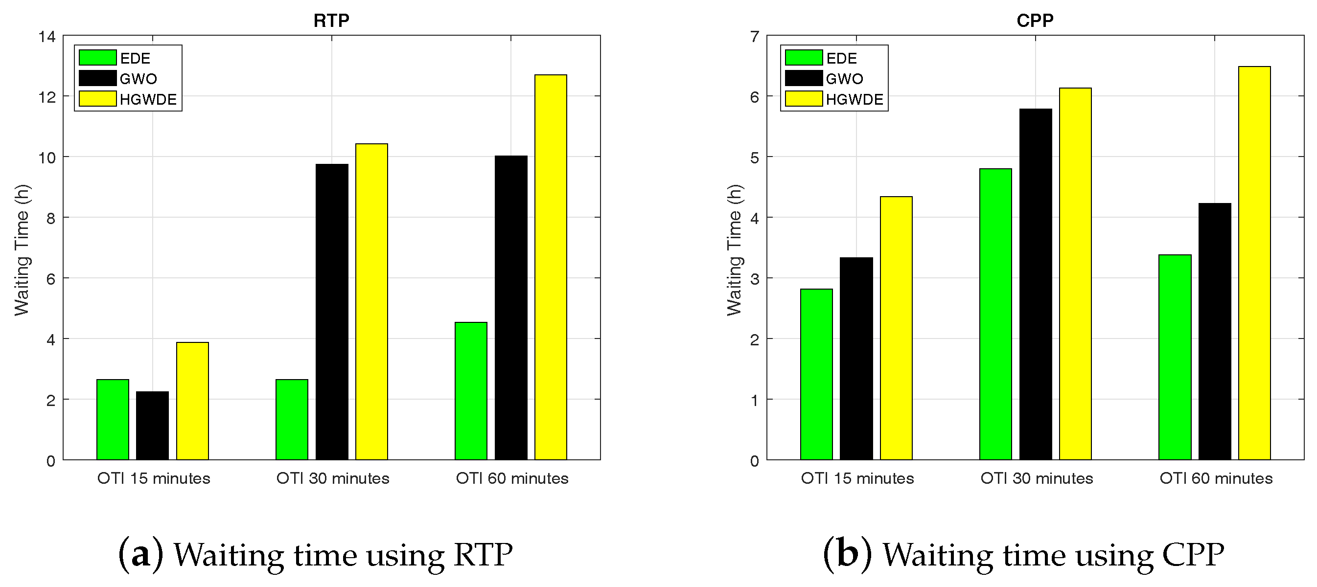
5.4. Waiting Time
5.4.1. Waiting Time Using RTP
5.4.2. Waiting time using CPP
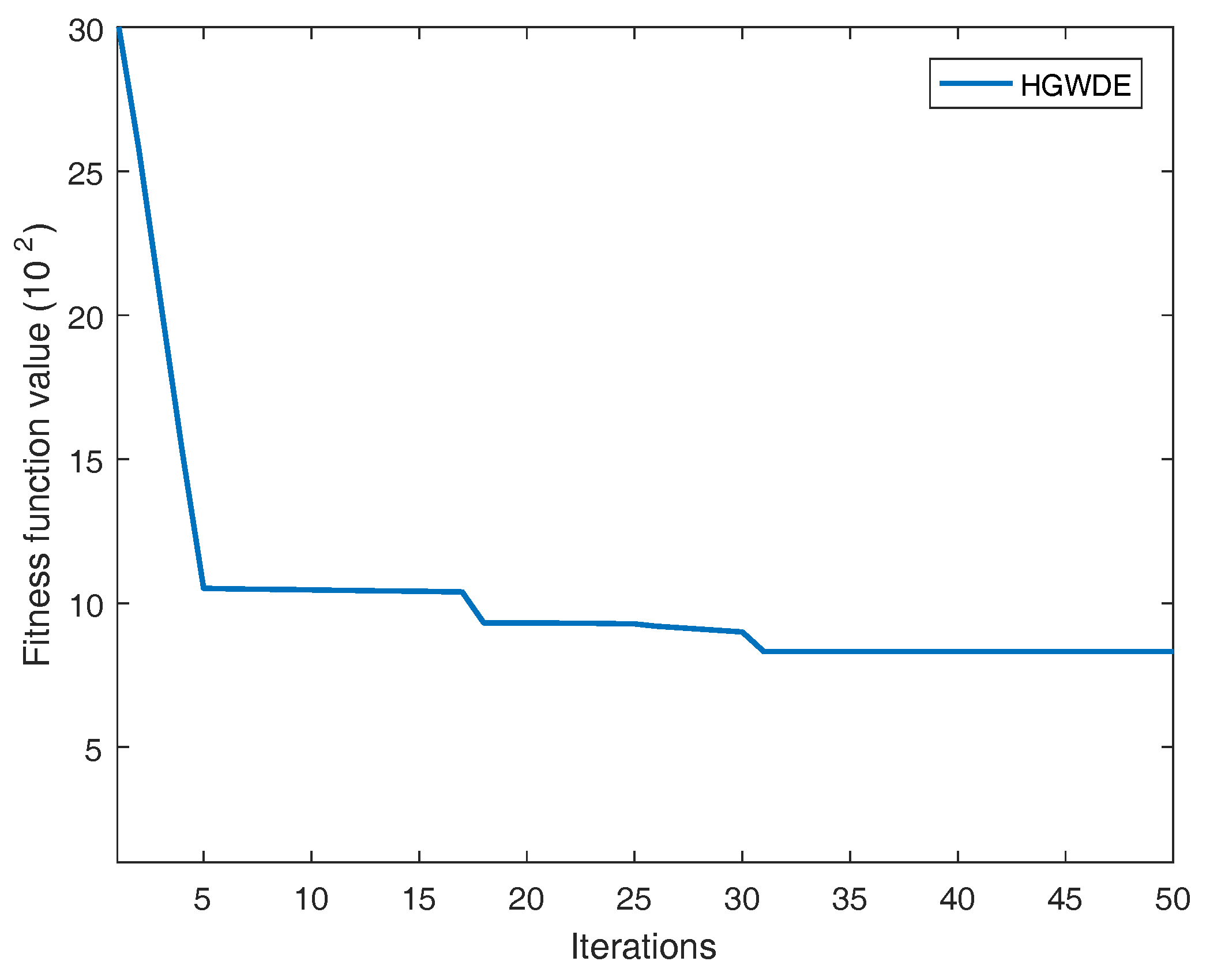
5.5. Convergence of the Fitness Function
5.6. Feasible Region
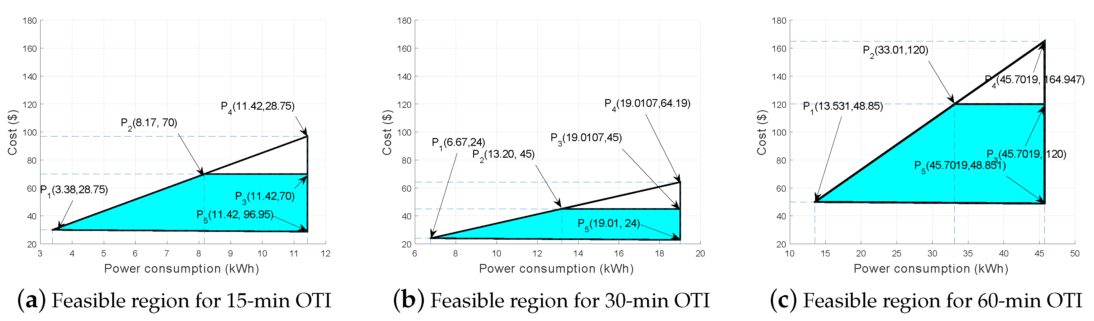
5.6.1. Feasible Region Using RTP
a. Feasible Region under 15-min OTI
b. Feasible Region under 30-min OTI
c. Feasible Region under 60-min OTI
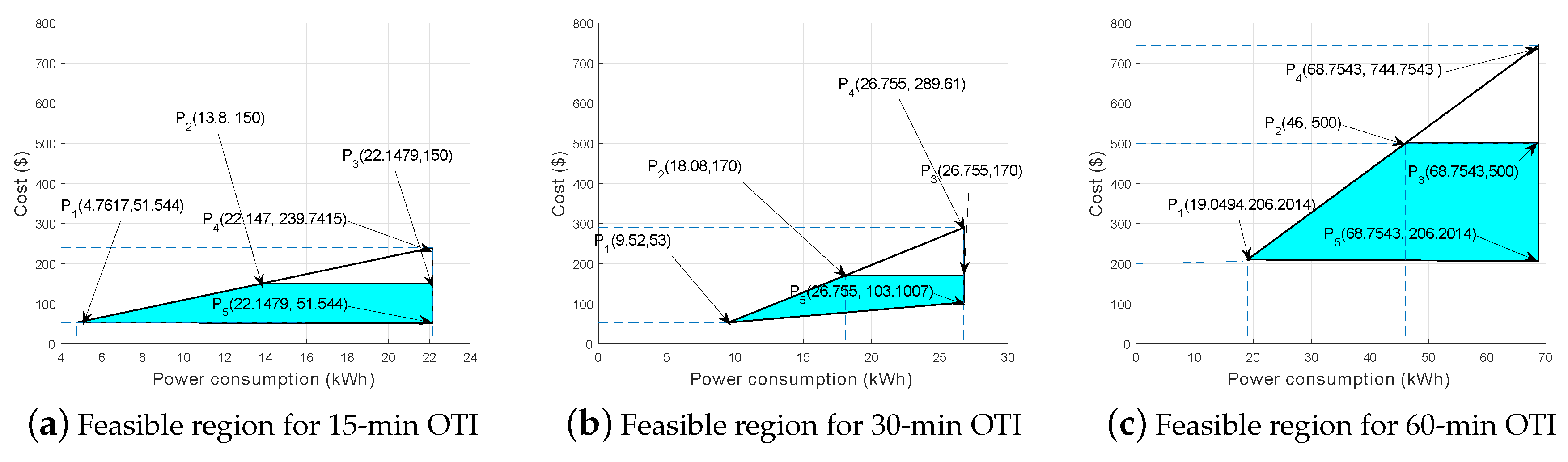
5.6.2. Feasible Region Using CPP
a. Feasible Region under 15-min OTI
b. Feasible Region under 30-min OTI
c. Feasible Region under 60-min OTI
5.7. Performance Trade-Off
6. Conclusions and Future Work
Acknowledgments
Author Contributions
Conflicts of Interest
References
- Mhanna, S.; Chapman, A.C.; Verbi, G. A fast distributed algorithm for large-scale demand response aggregation. IEEE Trans. Smart Grid 2016, 7, 2094–2107. [Google Scholar] [CrossRef]
- Energy Reports. Available online: http://www.enerdata.net/enerdatauk/press-and-publication/energy-features/enerfuture-2007.php (accessed on 1 August 2015).
- Logenthiran, T.; Srinivasan, D.; Shun, T.Z. Demand side management in smart grid using heuristic optimization. IEEE Trans. Smart Grid 2012, 3, 1244–1252. [Google Scholar] [CrossRef]
- Shirazi, E.; Jadid, S. Optimal residential appliance scheduling under dynamic pricing scheme via HEMDAS. Energy Build. 2015, 93, 40–49. [Google Scholar] [CrossRef]
- Bradac, Z.; Kaczmarczyk, V.; Fiedler, P. Optimal scheduling of domestic appliances via MILP. Energies 2014, 8, 217–232. [Google Scholar] [CrossRef]
- Teets, W. The association between stock market responses to earnings announcements and regulation of electric utilities. J. Account. Res. 1992, 30, 274–285. [Google Scholar] [CrossRef]
- Mahmood, A.; Javaid, N.; Khan, N.A.; Razzaq, S. An optimized approach for home appliances scheduling in smart grid. In Proceedings of the 2016 19th International Multi-Topic Conference (INMIC), Islamabad, Pakistan, 5–6 December 2016; pp. 1–5. [Google Scholar]
- Veras, J.M.; Pinheiro, P.R.; Silva, I.R.S.; Rabêlo, R.A. A Demand Response Optimization Model for Home Appliances Load Scheduling. In Proceedings of the 2017 IEEE International Conference on Systems, Man, and Cybernetics (SMC), Banff, AB, Canada, 5–8 October 2017. [Google Scholar]
- Ahmad, A.; Khan, A.; Javaid, N.; Hussain, H.M.; Abdul, W.; Almogren, A.; Alamri, A.; Azim Niaz, I. An Optimized Home Energy Management System with Integrated Renewable Energy and Storage Resources. Energies 2017, 10, 549. [Google Scholar] [CrossRef]
- Javaid, N.; Naseem, M.; Rasheed, M.B.; Mahmood, D.; Khan, S.A.; Alrajeh, N.; Iqbal, Z. A new heuristically optimized Home Energy Management controller for smart grid. Sustain. Cities Soc. 2017, 34, 211–227. [Google Scholar] [CrossRef]
- Rahimi, F.; Ipakchi, A. Demand response as a market resource under the smart grid paradigm. IEEE Trans. Smart Grid 2010, 1, 82–88. [Google Scholar] [CrossRef]
- Yang, H.T.; Yang, C.T.; Tsai, C.C.; Chen, G.J.; Chen, S.Y. Improved PSO based home energy management systems integrated with demand response in a smart grid. In Proceedings of the 2015 IEEE Congress on Evolutionary Computation (CEC), Sendai, Japan, 25–28 May 2015; pp. 275–282. [Google Scholar]
- Ogwumike, C.; Short, M.; Abugchem, F. Heuristic Optimization of Consumer Electricity Costs using a Generic Cost Model. Energies 2016, 9, 6. [Google Scholar] [CrossRef] [Green Version]
- Rasheed, M.B.; Javaid, N.; Ahmad, A.; Khan, Z.A.; Qasim, U.; Alrajeh, N. An efficient power scheduling scheme for residential load management in smart homes. Appl. Sci. 2015, 5, 1134–1163. [Google Scholar] [CrossRef]
- Tuaimah, F.M.; Abd, Y.N.; Hameed, F.A. Ant Colony Optimization based Optimal Power Flow Analysis for the Iraqi Super High Voltage Grid. Int. J. Comput. Appl. 2013, 67, 13–18. [Google Scholar]
- Logenthiran, T.; Srinivasan, D.; Vanessa, K.W.M. Demand side management of smart grid: Load shifting and incentives. J. Renew. Sustain. Energy 2014, 6, 033136. [Google Scholar] [CrossRef]
- Islam, S.M.; Das, S.; Ghosh, S.; Roy, S.; Suganthan, P.N. An adaptive differential evolution algorithm with novel mutation and crossover strategies for global numerical optimization. IEEE Trans. Syst. Man Cybern. Part B (Cybern.) 2012, 42, 482–500. [Google Scholar] [CrossRef] [PubMed]
- Li, H.; Zhang, Q. Multiobjective optimization problems with complicated Pareto sets, MOEA/D and NSGA-II. IEEE Trans. Evol. Comput. 2009, 13, 284–302. [Google Scholar] [CrossRef]
- Setlhaolo, D.; Xia, X. Optimal scheduling of household appliances incorporating appliance coordination. Energy Proc. 2014, 61, 198–202. [Google Scholar] [CrossRef]
- Osório, G.J.; Matias, J.C.O.; Catalão, J.P.S. Electricity prices forecasting by a hybrid evolutionary-adaptive methodology. Energy Convers. Manag. 2014, 80, 363–373. [Google Scholar] [CrossRef]
- Shayeghi, H.; Ghasemi, A.; Moradzadeh, M.; Nooshyar, M. Simultaneous day-ahead forecasting of electricity price and load in smart grids. Energy Convers. Manag. 2015, 95, 371–384. [Google Scholar] [CrossRef]
- Derakhshan, G.; Shayanfar, H.A.; Kazemi, A. The optimization of demand response programs in smart grids. Energy Policy 2016, 94, 295–306. [Google Scholar] [CrossRef]
- Soares, J.; Ghazvini, M.A.F.; Vale, Z.; de Moura Oliveira, P.B. A multi-objective model for the day-ahead energy resource scheduling of a smart grid with high penetration of sensitive loads. Appl. Energy 2016, 162, 1074–1088. [Google Scholar] [CrossRef]
- Ghasemi, A.; Shayeghi, H.; Moradzadeh, M.; Nooshyar, M. A Novel hybrid algorithm for electricity price and load forecasting in smart grids with demand-side management. Appl. Energy 2016, 177, 40–59. [Google Scholar] [CrossRef]
- Jayabarathi, T.; Raghunathan, T.; Adarsh, B.R.; Suganthan, P.N. Economic dispatch using hybrid grey wolf optimizer. Energy 2016, 111, 630–641. [Google Scholar] [CrossRef]
- Lugo-Cordero, H.M.; Fuentes-Rivera, A.; Guha, R.K.; Ortiz-Rivera, E.I. Particle swarm optimization for load balancing in green smart homes. In Proceedings of the 2011 IEEE Congress of Evolutionary Computation(CEC), New Orleans, LA, USA, 5–8 June 2011; pp. 715–720. [Google Scholar]
- Geem, Z.W.; Kim, J.H.; Loganathan, G.V. A new heuristic optimization algorithm: Harmony 578 search. Simulation 2001, 76, 60–68. [Google Scholar] [CrossRef]
- Storn, R.; Price, K. Differential Evolution—A Simple and Efficient Adaptive Scheme for Global 580 Optimization over Continuous Spaces; International Computer Science Institute: Berkeley, CA, USA, 1995. [Google Scholar]
- Vardakas, J.S.; Zorba, N.; Verikoukis, C.V. Performance evaluation of power demand scheduling scenarios in a smart grid environment. Appl. Energy 2015, 142, 164–178. [Google Scholar] [CrossRef]
- Yi, P.; Dong, X.; Iwayemi, A.; Zhou, C.; Li, S. Real-time opportunistic scheduling for residential demand response. IEEE Trans. Smart Grid 2013, 4, 227–234. [Google Scholar] [CrossRef]
- Yuce, B.; Rezgui, Y.; Mourshed, M. ANN–GA smart appliance scheduling for optimised energy management in the domestic sector. Energy Build. 2016, 111, 311–325. [Google Scholar] [CrossRef]
- Reka, S.S.; Ramesh, V. A demand response modeling for residential consumers in smart grid environment using game theory based energy scheduling algorithm. Ain Shams Eng. J. 2016, 7, 835–845. [Google Scholar] [CrossRef]
- Erdinc, O. Economic impacts of small-scale own generating and storage units, and electric vehicles under different demand response strategies for smart households. Appl. Energy 2014, 126, 142–150. [Google Scholar] [CrossRef]
- Agnetis, A.; de Pascale, G.; Detti, P.; Vicino, A. Load scheduling for household energy consumption optimization. IEEE Trans. Smart Grid 2013, 4, 2364–2373. [Google Scholar] [CrossRef]
- Setlhaolo, D.; Xia, X.; Zhang, J. Optimal scheduling of household appliances for demand response. Electr. Power Syst. Res. 2014, 116, 24–28. [Google Scholar] [CrossRef]
- Pradhan, M.; Roy, P.K.; Pal, T. Grey wolf optimization applied to economic load dispatch problems. Int. J. Electr. Power Energy Syst. 2016, 83, 325–334. [Google Scholar] [CrossRef]
- Javaid, N.; Ullah, I.; Akbar, M.; Iqbal, Z.; Khan, F.A.; Alrajeh, N.; Alabed, M.S. An intelligent load management system with renewable energy integration for smart homes. IEEE Access 2017, 5, 13587–13600. [Google Scholar] [CrossRef]
- Vardakas, J.S.; Zorba, N.; Verikoukis, C.V. Power demand control scenarios for smart grid applications with finite number of appliances. Appl. Energy 2016, 162, 83–98. [Google Scholar] [CrossRef]
- Ogunjuyigbe, A.S.O.; Ayodele, T.R.; Akinola, O.A. User satisfaction-induced demand side load management in residential buildings with user budget constraint. Appl. Energy 2017, 187, 352–366. [Google Scholar] [CrossRef]
- Singh, N.; Singh, S.B. Hybrid Algorithm of Particle Swarm Optimization and Grey Wolf Optimizer for Improving Convergence Performance. J. Appl. Math. 2017, 2017, 2030489. [Google Scholar] [CrossRef]
- Waterloo North Hydro. Available online: https://www.wnhydro.com/en/your-home/time-of-use-rates.asp (accessed on 6 December 2017).
- Muralitharan, K.; Sakthivel, R.; Shi, Y. Multiobjective optimization technique for demand side management with load balancing approach in smart grid. Neurocomputing 2016, 177, 110–119. [Google Scholar] [CrossRef]


| DSM | Demand side management |
| GWO | Gray wolf optimization |
| EDE | Enhanced differential evaluation |
| HGWDE | Hybrid gray wolf differential evaluation |
| BFA | Bacterial foraging optimization |
| PSO | Particle swarm optimization |
| BPSO | Binary particle swarm optimization |
| TLBO | Teaching- and learning-based optimization |
| IDSS | Intelligent decision support system |
| MOO | Multi-objective optimization |
| AMI | Advanced metering infrastructure |
| EMC | Energy management controller |
| LOT | Length of operational time |
| HEM | Home energy management |
| RTP | Real-time pricing |
| CPP | Critical peak pricing |
| OTI | Operational time interval |
| RES | Renewable energy sources |
| DR | Demand response |
| WDO | Wind-driven optimization |
| TOU | Time of use |
| FRP | Flat rate pricing |
| IBR | Inclined block rate |
| DHP | Day-ahead pricing |
| PS | Pareto sets |
| SG | Smart grid |
| SM | Smart meter |
| GA | Genetic algorithm |
| SFL | Shuffled frog leaping |
| D | Total appliances |
| Set of shiftable appliances | |
| Set of controllable appliances | |
| Set of non-shiftable appliances | |
| Power rating | |
| Status of appliance | |
| h | Time slots |
| Trial vector | |
| Mutant vector | |
| Upper bound | |
| Lower bound | |
| Crossover rate | |
| Population | |
| Maximum iteration | |
| Position of the search agent | |
| Position of the search agent | |
| Position of the search agent | |
| F | Scaling factor |
| Fitness coefficients | |
| Best search agent | |
| Second best optimal solution | |
| Third best optimal solution |
| Features | Techniques | Targets Achieved | Limitations |
|---|---|---|---|
| MILP | Optimal scheduling of domestic appliances [5] | Minimize cost | Ignored user comfort |
| Greedy algorithm | Heuristic optimization of consumer electricity costs using a generic cost model [13] | Minimized user frustration and cost | PAR is ignored, system complexity increased |
| Multi-agent model | Demand-side management of the smart grid: load shifting and incentives [16] | Load shifting and cost minimization | User comfort is compromised |
| BPSO and neuro-fuzzy logic | Electricity price forecasting by a hybrid evolutionary-adaptive methodology [21] | Electricity market price forecasting using mean absolute percentage error (MAPE) | Trade-off between MAPE and computational time |
| Multiple input multiple output model (MIMO) | Simultaneous day-ahead forecasting of electricity price and load in smart grids [22] | Load and price signal forecasting | Real-time forecasting is not considered |
| Teaching and learning-based optimization (TLBO) and shuffled frog leaping (SFL) | The optimization of demand response programs in smart grids [23] | Cost optimization | RES not integrated |
| PSO and MILP | A multi-objective model for the day-ahead energy resource scheduling of a smart grid with high penetration of sensitive loads [24] | Virtual power play scheduling | Requirements of the customers for reliable power grids is not considered |
| MIMO | Novel hybrid algorithm for electricity price and load forecasting in smart grids with demand-side management [25] | Electricity price and load forecasting | Computational time is not practical |
| GWO | Economic dispatch using the hybrid gray wolf optimizer [31] | Solving non-linear economic load dispatch problems | The user has to come up with ways of handling the constraints |
| ANN-GA | ANN-GA smart appliance scheduling for optimized energy management in the domestic sector [32] | Reduction in grid energy usage | Cannot be applied to different building types involving a higher number of appliances |
| Game theory algorithm (GTFT) | A demand response modeling for residential consumers in a smart grid environment using a game theory-based energy scheduling algorithm [33] | Scheduling the appliances using the game theory strategy and PAR reduction | RES not integrated |
| MILP and heuristic algorithms | Load scheduling for household energy consumption optimization [34] | Load balancing | Cost minimization is not considered |
| MINLP | Optimal scheduling of household appliances for demand response [35] | Cost reduction is achieved | PAR is ignored |
| GWO and ILP | Grey wolf optimization applied to economic load dispatch problems [36] | Load dispatching in off-peak hours | Solved economic load dispatch (ELD) problems in the current study |
| Appliance Class | Appliance | Power | Earliest Starting | Finishing | LOT (h) |
|---|---|---|---|---|---|
| Rating (kWh) | Time (h) | Time (h) | |||
| Shiftable Appliances | Washing Machine | 1.4 | 6 | 10 | 1–3 |
| Dish Washer | 1.32 | 15 | 20 | 1–3 | |
| Hair Straightener | 0.055 | 18 | 8 | 1–2 | |
| Hair Dryer | 1.8 | 18 | 8 | 1–2 | |
| Microwave | 1.2 | 18 | 8 | 3–5 | |
| Telephone | 0.005 | 9 | 17 | 1–24 | |
| Computer | 0.15 | 18 | 24 | 6–12 | |
| Oven | 2.4 | 6 | 10 | 1–3 | |
| Cooker | 0.225 | 18 | 24 | 2–4 | |
| Iron | 2.4 | 18 | 24 | 3–5 | |
| Toaster | 0.8 | 9 | 17 | 1–2 | |
| Kettle | 2 | 18 | 8 | 1–2 | |
| Printer | 0.011 | 18 | 24 | 1–2 | |
| Non-Shiftable Appliances | Television | 0.083 | 9 | 17 | 6–12 |
| Refrigerator | 1.666 | 1 | 24 | 1–24 | |
| Controllable Appliances | Air Conditioner | 1.14 | 16 | 24 | 6–8 |
| Lightning | 0.1 | 1 | 24 | 12–20 |
| EDE Parameters | HEM Parameters | Values |
|---|---|---|
| Population Number of dimensions Gradient of problem | Possible solution Number of appliances Scheduling | 50 17 vary |
| HGWDE Parameters | HEM Parameters | Values |
|---|---|---|
| Population Wolfs in each pack Minimum distance from prey Status of leader | Possible solution Appliances Min (cost) status of appliance | 50 17 vary 1 or 0 |
| Techniques | Cost (Cents) Using RTP | Cost (Cents) Using CPP | ||||
|---|---|---|---|---|---|---|
| 15 min | 30 min | 60 min | 15 min | 30 min | 60 min | |
| Unscheduled | 500.4826 | 743.4876 | 822.1562 | 1200.1562 | 1300.890 | 1085.648 |
| EDE | 420.5380 | 743.1959 | 831.2135 | 1178.0462 | 1164.490 | 1190.690 |
| GWO | 426.0507 | 727.1436 | 717.9405 | 1190.5123 | 1200.96 | 1080.409 |
| HGWDE | 416.7467 | 658.6506 | 712.7298 | 1164.490 | 1085.90 | 1056.7890 |
| Techniques | PAR Using RTP with Multiple OTIs | PAR Using CPP with Multiple OTIs | ||||
|---|---|---|---|---|---|---|
| 15 min | 30 min | 60 min | 15 min | 30 min | 60 min | |
| Unscheduled | 10.9697 | 6.0257 | 5.0257 | 10.9697 | 5.8034 | 5.0257 |
| EDE | 8.1722 | 5.8424 | 3.6558 | 8.1722 | 5.2536 | 3.8424 |
| GWO | 5.675 | 5.9335 | 4.3509 | 5.626 | 4.8165 | 3.9335 |
| HGWDE | 5.1530 | 3.6209 | 2.5369 | 5.5415 | 4.0263 | 3.6209 |
| Techniques | Waiting Time Using RTP with Multiple OTIs | Waiting Time Using CPP with Multiple OTIs | ||||
|---|---|---|---|---|---|---|
| 15 min | 30 min | 60 min | 15 min | 30 min | 60 min | |
| EDE | 4.3781 h | 4.5394 h | 2.6560 h | 3.3826 h | 4.8012 h | 2.8158 h |
| GWO | 9.7494 h | 10.0262 h | 2.2397 h | 4.2293 h | 5.7853 h | 3.3346 h |
| HGWDE | 10.4249 h | 12.7007 h | 3.8793 h | 6.4814 h | 6.1335 h | 4.3408 h |
| Cases | Price (Cents) | Load (kWh) | Cost (Cents) |
|---|---|---|---|
| Min Price, Min Load Min Price, Max Load Max Price, Min Load Max Price, Max Load | 8.100 8.100 27.35 27.35 | 0.4177 3.54 0.4177 3.54 | 3.38 28.75 11.42 96.95 |
| Cases | Price (Cents) | Load (kWh) | Cost (Cents) |
|---|---|---|---|
| Min Price, Min Load Min Price, Max Load Max Price, Min Load Max Price, Max Load | 8.100 8.100 27.35 27.35 | 0.8355 2.34 0.8355 2.34 | 6.76 19.0107 22.8509 69.1904 |
| Cases | Price (Cents) | Load (kWh) | Cost (Cents) |
|---|---|---|---|
| Min Price, Min Load Min Price, Max Load Max Price, Min Load Max Price, Max Load | 8.100 8.100 27.35 27.35 | 1.67 6.03 1.67 6.03 | 13.531 45.7019 48.851 164.947 |
| Cases | Price (Cents) | Load (kWh) | Cost (Cents) |
|---|---|---|---|
| Min Price, Min Load Min Price, Max Load Max Price, Min Load Max Price, Max Load | 11.4 11.4 123.4 123.4 | 0.4177 1.9428 0.4177 1.9428 | 4.76178 22.14792 51.544 239.74152 |
| Cases | Price (Cents) | Load (kWh) | Cost (Cents) |
|---|---|---|---|
| Min Price, Min Load Min Price, Max Load Max Price, Min Load Max Price, Max Load | 11.4 11.4 123.4 123.4 | 0.8355 2.3470 0.8355 2.3470 | 9.5247 26.7558 103.1007 289.6198 |
| Cases | Price (Cents) | Load (kWh) | Cost (Cents) |
|---|---|---|---|
| Min Price, Min Load Min Price, Max Load Max Price, Min Load Max Price, Max Load | 11.4 11.4 123.4 123.4 | 1.6710 6.0310 1.6710 6.0310 | 19.0494 68.7534 206.2014 744.2254 |
© 2018 by the authors. Licensee MDPI, Basel, Switzerland. This article is an open access article distributed under the terms and conditions of the Creative Commons Attribution (CC BY) license (http://creativecommons.org/licenses/by/4.0/).
Share and Cite
Naz, M.; Iqbal, Z.; Javaid, N.; Khan, Z.A.; Abdul, W.; Almogren, A.; Alamri, A. Efficient Power Scheduling in Smart Homes Using Hybrid Grey Wolf Differential Evolution Optimization Technique with Real Time and Critical Peak Pricing Schemes. Energies 2018, 11, 384. https://doi.org/10.3390/en11020384
Naz M, Iqbal Z, Javaid N, Khan ZA, Abdul W, Almogren A, Alamri A. Efficient Power Scheduling in Smart Homes Using Hybrid Grey Wolf Differential Evolution Optimization Technique with Real Time and Critical Peak Pricing Schemes. Energies. 2018; 11(2):384. https://doi.org/10.3390/en11020384
Chicago/Turabian StyleNaz, Muqaddas, Zafar Iqbal, Nadeem Javaid, Zahoor Ali Khan, Wadood Abdul, Ahmad Almogren, and Atif Alamri. 2018. "Efficient Power Scheduling in Smart Homes Using Hybrid Grey Wolf Differential Evolution Optimization Technique with Real Time and Critical Peak Pricing Schemes" Energies 11, no. 2: 384. https://doi.org/10.3390/en11020384