A Novel Stochastic-Programming-Based Energy Management System to Promote Self-Consumption in Industrial Processes

Abstract

The introduction of non-conventional energy sources (NCES) to industrial processes is a viable alternative to reducing the energy consumed from the grid. However, a robust coordination of the local energy resources with the power imported from the distribution grid is still an open issue, especially in countries that do not allow selling energy surpluses to the main grid. In this paper, we propose a stochastic-programming-based energy management system (EMS) focused on self-consumption that provides robustness to both sudden NCES or load variations, while preventing power injection to the main grid. The approach is based on a finite number of scenarios that combines a deterministic structure based on spectral analysis and a stochastic model that represents variability. The parameters to generate these scenarios are updated when new information arrives. We tested the proposed approach with data from a copper extraction mining process. It was compared to a traditional EMS with perfect prediction, i.e., a best case scenario. Test results show that the proposed EMS is comparable to the EMS with perfect prediction in terms of energy imported from the grid (slightly higher), but with less power changes in the distribution side and enhanced dynamic response to transients of wind power and load. This improvement is achieved with a non-significant computational time overload.

1. Introduction

In recent years, the integration of non-conventional energy sources (NCES) into the distribution networks has became an interesting area of research in power systems. The design of energy management systems (EMS) is one of the most widely studied topics within this area due to its crucial contribution in the attempt of keeping the load-generation balance in the network. An EMS is a control system that aims to reduce as much as possible the operating costs of a network with both multiple energy sources and high penetration of NCES (which is the case of micro-grids), while maintaining its reliable operation. This is performed through the dispatch and commitment of those generation units that can be scheduled throughout the day (e.g., energy storage systems and diesel generators). Since the objective is to reduce the operating costs, the energy management problem is often formulated as an minimization problem. Given the predicted contributions of the NCES, the estimated load, and the reserve requirements in the network, the solution of the energy management problem assigns to each generation unit (that can be scheduled) the amount of power that they have to provide [1]. Such scheduling of the generation units defines the interaction among local demand, local energy sources, and the distribution network, by determining the amount of energy that must be imported/exported from the distribution system, for instance depending on the non-conventional energy availability. Therefore, an EMS has many possible uses in distribution grids, for example in coordinating among local generation resources so that the local demand is supplied with an optimal use of the available infrastructure [2,3,4]. They have also been investigated as a potential alternative for reducing the loses of distribution systems through the integration of NCES in different contexts such as homes, buildings, and energy hubs [5,6,7].

However, the performance of an EMS highly depends on how the uncertainty of the NCES, the energy prices, and the load is addressed in the formulation of the corresponding optimization problem. An alternative for addressing the uncertainty of those variables in the formulation of the energy management problem is the use of uncertainty models. The idea behind this alternative is to integrate the differences that could appear between the model used in the optimization-based EMS and the real system. Then, the solution obtained will be robust against any realization of the uncertain variables that can be represented by the model used in the formulation. In the specialized literature, different methods have been proposed to model the uncertainty in the energy management problem [8,9]. Depending on the uncertainty modeling, these approaches were classified as stochastic or robust [8,10,11,12]. In the former, probability density functions (p.d.f) were used to generate possible realizations of the uncertain variables. Based on these realizations, a solution of the energy management problem that satisfies all constraints in all considered realizations is obtained [13]. In [14], for instance, a specific application of the stochastic EMS was presented. In this approach, a p.d.f was obtained for each uncertain variable and a set of realizations for each variable was conformed. From this set, the EMS decided the amount of power of each generation unit in the network. By contrast, in the robust approach it is assumed that the uncertain variables evolve within a defined set. Often, ellipsoids and polytopes are used to approximate such a set. The obtained solution of the energy management problem satisfies all constraints for any realization of the uncertain variables within the defined uncertainty set [13]. In [15], an application of the robust EMS was presented. In this particular application, the uncertainty sets evolved with time. That is, at each sample time the parameters of the uncertainty sets were computed, and then the energy management problem was solved. This increases the complexity of the EMS but might reduce its conservativeness. Other approaches of stochastic and robust EMS were proposed in [9,16,17]. In these cases, the EMS was applied in transmission networks as part of a multi-stage approach for operation with different degrees of uncertainty (e.g., in the price-elastic demand curve).

Although the use of robust- and stochastic-programming-based EMS at transmission and distribution levels demonstrated their effectiveness on allowing a massive integration of NCES in the operation of power grids at different scales (e.g., from micro-grids to bulk power grids, and from distribution to transmission networks), little attention has been paid to their use in promoting the self-consumption. Focusing on self-consumption is important because there are several countries worldwide that forbid that small electric energy producers inject their energy surpluses into the distribution grid. Some examples of these countries are Colombia, Norway, Paraguay, Saudi Arabia and another 37 countries according to [18]. Furthermore, countries (like Chile) in which small electric energy producers are allowed to inject their energy surpluses into the distribution network are experiencing congestion and voltage issues at the distribution level. An alternative to overcome these issues (without reducing the penetration rate of NCES) is focusing on promoting self-consumption.

The present paper presents a stochastic-programming-based EMS for applications with self-consumption. To guarantee that the injection of energy surpluses is minimized, additional constraints are included as well as terms to avoid as much as possible the effects of energy curtailment of NCES. Moreover, in the proposed EMS we use a limited set of synthetically generated prediction scenarios. These scenarios are generated using a model obtained from an analysis of the historical data of the uncertain variables. This model combines a deterministic structure obtained from a spectral analysis and a random structure that allows generating different prediction scenarios of the uncertain variables, such as non-conventional energy resources and local power demand. The number of scenarios used at each execution of the EMS is computed based on the mean and variance of the empirical probability density function (e.p.d.f) of the uncertain variables. Since the e.p.d.f of the uncertain variables is used to generate the scenarios, its mean and variance are updated with the new measured values of the corresponding variable. Thus, an adaptation structure is obtained in which more scenarios are generated when uncertain variables exhibit more variability. Furthermore, since the industrial sector is the most pollutant end-user sector [19], a special emphasis has been done in this kind of applications. Indeed, the IEEE (Institute of Electrical and electronics Engineers) nine-busbars system was adapted to simulate an equivalent grid of a typical copper mine with co-generation. The obtained results show that the proposed EMS allows for significantly reducing the injection of energy surpluses in comparison with a conventional EMS strategy, while maximizing the use of NCES to satisfy the local demand and minimize the effects of energy curtailment of the NCES. The remainder of this paper is organized as follows: Section 2 presents the formulation of the proposed EMS; Section 3 shows the case study and the simulation results; and Section 4 presents the concluding remarks.

2. Proposed Stochastic Energy Management System

On the current investigation, we formulate a novel stochastic-programing-based EMS for NCES applications oriented to promote self-consumption. In particular, the industrial case is analyzed since the demand is almost predictable based on the scheduling of the machines involved in the process (the uncertainty in the industrial demand is mainly due to variation in the quality of the raw materials). On industrial processes, the coincidence between energy availability and demand is higher than residential load centers; then, the effect of self-consumption policies is higher in industries than in homes, and the possibility of having co-generation allows avoiding the necessity of a battery storage system that increases the investment costs to around 20% [20] of the total cost of the NCES application. In addition, the massive inclusion of batteries in NCES application implies some environmental consequences. For instance, the world scarcity of lithium is an issue, as it is currently the most commonly used raw material for battery manufacturing. Indeed, it has been estimated that if developing countries use lithium at the same rate as developed countries, the amounts required of this mineral could be up to nine times as much as we currently globally use. On the other hand, production of lithium batteries has the most significant contribution to greenhouse gases, CO₂, demanded energy (24.4 KWh per Kg) and metal depletion compared to other battery manufacturing materials such as lead acid and nickel cadmium [21]. Nonetheless, the proposed EMS could be easily extended to consider applications that combine both energy storage systems and NCES such as residential applications to promote self-consumption. The mathematical framework presented in [22] was used to formulate the proposed EMS. Our approach additionally considers a rolling horizon that requires updating the prediction of the uncertain variables at every sample-time. Based on this, a prediction model of each uncertain variable was derived based on historical datasets. Furthermore, these datasets were also used to determine the probability of occurrence of each realization of the uncertain models generated with the prediction models. This mathematical framework was selected because it is possible to derive a tractable worst-case scenario formulation for the resulting optimization problem.

In addition to the uncertainty representation, one of the main concerns regarding current EMS approaches is the use of single-node representations of the distribution system. With this representation, it cannot be guaranteed that the scheduled power could be transmitted to the load centers in a secure way. However, since the EMS proposed in this paper is focused on industrial applications of NCES, it can be assumed that the internal energy system is designed in accordance to the demand requirements, that the losses are not significant since the electric system is circumscribed to a relatively small area, and that the distribution system behaves as a source/sink of energy. Then, the single-node representation of the distribution system is adequate for this kind of application.

2.1. EMS Formulation

For a given industrial process, let $N_{\mathrm{p}}$ denote the prediction horizon. At time step k, let $P_{\mathrm{r}j}\left(k\right)$ denote the real power generated by the j-th NCES ($j=1,\dots ,N$); $P_{\mathrm{d}o}\left(k\right)$ denotes the real power demanded by the o-th load center/process ($o=1,\dots ,O$); $P_{\mathrm{g}i}\left(k\right)$ and $C_{\mathrm{g}i}$ respectively denote the real power generated by the i-th co-generation source and its corresponding generation cost ($i=1,\dots ,M$); $P_{\mathrm{ns}}\left(k\right)$ and $C_{\mathrm{ns}}$ respectively denote the non-supplied energy and its corresponding cost; $P_{\mathrm{lo}}\left(k\right)$ and $C_{\mathrm{lo}}$ respectively denote the lost energy and its corresponding cost; and $P_{\mathrm{dist}}\left(k\right)$ and $C_{\mathrm{dist}}\left(k\right)$ respectively denote the real power imported from the distribution grid and its corresponding cost. Then, the optimization problem associated with the proposed EMS is given by:

$$\begin{array}{c}\underset{\begin{array}{c}{P}_{\mathrm{dist}}\left(k\right),P_{\mathrm{g}i}\left(k\right),\\ P_{\mathrm{ns}}\left(k\right),P_{\mathrm{lo}}\left(k\right)\end{array}}{min}\sum _{k=1}^{N_{\mathrm{p}}}\left[C_{\mathrm{dist}}\left(k\right)P_{\mathrm{dist}}\left(k\right)+\sum _i^M{C}_{\mathrm{g}i}{P}_{\mathrm{g}i}\left(k\right)+C_{\mathrm{ns}}{P}_{\mathrm{ns}}\left(k\right)+C_{\mathrm{lo}}{P}_{\mathrm{lo}}\left(k\right)\right]\hfill \\ \mathbf{s}.\mathbf{t}:\hfill \\ P_{\mathrm{dist}}\left(k\right)+\sum _{i=1}^M{P}_{\mathrm{g}i}\left(k\right)+\sum _{j=1}^N{P}_{\mathrm{r}j}\left(k\right)+P_{\mathrm{ns}}\left(k\right)=\sum _{o=1}^O{P}_{\mathrm{d}o}\left(k\right)+P_{\mathrm{lo}}\left(k\right),k=1,\dots ,N_{\mathrm{p}}\hfill \\ P_{\mathrm{g}i}^{\min }\le P_{\mathrm{g}i}\left(k\right)\le P_{\mathrm{g}i}^{\max },i=1,\dots ,M;k=1,\dots ,N_{\mathrm{p}}\hfill \\ P_{\mathrm{dist}}\left(k\right)\ge 0,P_{\mathrm{ns}}\left(k\right)\ge 0,P_{\mathrm{lo}}\left(k\right)\ge 0,k=1,\dots ,N_{\mathrm{p}}\hfill \end{array}$$

(1)

with $P_{\mathrm{g}i}^{\min }$ and $P_{\mathrm{g}i}^{\max }$ the minimum and maximum real power generation capacity of co-generation source i, respectively. Note that in Equation (1) both $P_{\mathrm{ns}}\left(k\right)$ and $P_{\mathrm{lo}}\left(k\right)$ are used to relax the power balance constraint; that the generation costs of co-generation units are assumed constant but their variation with time (e.g., due to the availability of primary energy sources) could be easily included in the formulation; that the additional constraint $P_{\mathrm{dist}}\left(k\right)\ge 0$ has been added to prevent injecting power to the distribution grid and therefore to promote the self-consumption; and that the uncertainties come from the price of the energy imported form the distribution network, the power generated by the NCES, and the demand. In the practice, these variables highly determine the scheduling of the generation units, but they are highly uncertain and therefore the uncertainty has to be accounted for in the energy management problem. In this paper, we derive a stochastic-programming formulation for the energy management problem Equation (1) following the procedure explained in [22].

2.2. Stochastic Robust Formulation

Let us assume that the uncertain variables are independent to each other, i.e., $C_{\mathrm{dist}}\left(k\right)$, $P_{\mathrm{r}j}\left(k\right)$, and $P_{\mathrm{d}o}\left(k\right)$ are independent stochastic processes. Then, a model for each variable could be derived so that a set of synthetic series is generated. At time step k, let $S\left(k\right)$ denote the number of series generated for each uncertain variable; let ${\Gamma }_{\mathrm{dist}}\left(k\right):=\{{\tilde{C}}_{\mathrm{dist}}^1\left(k\right),\dots ,{\tilde{C}}_{\mathrm{dist}}^{S\left(k\right)}\left(k\right)\}$, ${\Gamma }_{\mathrm{r}j}\left(k\right):=\{{\tilde{P}}_{\mathrm{r}j}^1\left(k\right),\dots ,{\tilde{P}}_{\mathrm{r}j}^{S\left(k\right)}\left(k\right)\}$ ($j=1,\dots ,N$), and ${\Gamma }_{\mathrm{d}o}\left(k\right):=\{{\tilde{P}}_{\mathrm{d}o}^1\left(k\right),\dots ,{\tilde{P}}_{\mathrm{d}o}^{S\left(k\right)}\left(k\right)\}$ ($o=1,\dots ,O$) denote the sets of synthetic series for the energy price, the power generated by each NCES, and the power demanded by each load center, respectively, with ${\tilde{C}}_{\mathrm{dist}}^q\left(k\right)$, ${\tilde{P}}_{\mathrm{r}j}^q\left(k\right)$, and ${\tilde{P}}_{\mathrm{d}o}^q\left(k\right)$ series of longitude $N_{\mathrm{p}}$ ($q=1,\dots ,S\left(k\right)$); and let ${\mathrm{\Xi }}_{\mathrm{dist}}\left(k\right):=\{{\xi }_{\mathrm{dist}}^1\left(k\right),\dots ,{\xi }_{\mathrm{dist}}^{S\left(k\right)}\left(k\right)\}$, ${\mathrm{\Xi }}_{\mathrm{r}j}\left(k\right):=\{{\xi }_{\mathrm{r}j}^1\left(k\right),\dots ,{\xi }_{\mathrm{r}j}^{S\left(k\right)}\left(k\right)\}$, and ${\mathrm{\Xi }}_{\mathrm{d}o}\left(k\right):=\{{\xi }_{\mathrm{d}o}^1\left(k\right),\dots ,{\xi }_{\mathrm{d}o}^{S\left(k\right)}\left(k\right)\}$, denote the set of probabilities of occurrence of each synthetic series for the energy price, the power generated by each NCES, and the power demanded by each load center, respectively, with ${\sum }_{q=1}^{S\left(k\right)}{\xi }_{\mathrm{dist}}^q\left(k\right)=1$, ${\sum }_{q=1}^{S\left(k\right)}{\xi }_{\mathrm{r}j}^q\left(k\right)=1$ ($j=1,\dots ,N$), and ${\sum }_{q=1}^{S\left(k\right)}{\xi }_{\mathrm{d}o}^q\left(k\right)=1$ ($o=1,\dots ,O$). Then, a scenario q is defined as the tuple ${\phi }^q\left(k\right):=({\tilde{C}}_{\mathrm{dist}}^q\left(k\right),{\tilde{P}}_{\mathrm{r}1}^q\left(k\right),\dots ,{\tilde{P}}_{\mathrm{r}N}^q\left(k\right),{\tilde{P}}_{\mathrm{d}1}^q\left(k\right),\dots ,{\tilde{P}}_{\mathrm{d}O}^q\left(k\right))$, with probability of occurrence ${\mu }^q\left(k\right)={\xi }_{\mathrm{dist}}^q\left(k\right)({\mathrm{\Pi }}_{j=1}^N{\xi }_{\mathrm{r}j}^q\left(k\right))({\mathrm{\Pi }}_{o=1}^O{\xi }_{\mathrm{d}o}^q\left(k\right))$.

For illustrative purposes, consider a NCES application with two NCES, two load centers, and two scenarios. According to the previous definitions, each scenario is given by ${\phi }^1\left(k\right)=({\tilde{C}}_{\mathrm{dist}}^1\left(k\right),{\tilde{P}}_{\mathrm{r}1}^1\left(k\right),{\tilde{P}}_{\mathrm{r}2}^1\left(k\right),{\tilde{P}}_{\mathrm{d}1}^1\left(k\right),{\tilde{P}}_{\mathrm{d}2}^1\left(k\right))$ and ${\phi }^2\left(k\right)=({\tilde{C}}_{\mathrm{dist}}^2\left(k\right),{\tilde{P}}_{\mathrm{r}1}^2\left(k\right),{\tilde{P}}_{\mathrm{r}2}^2\left(k\right),{\tilde{P}}_{\mathrm{d}1}^2\left(k\right),{\tilde{P}}_{\mathrm{d}2}^2\left(k\right))$, with probabilities of occurrence ${\mu }^1\left(k\right)={\xi }_{\mathrm{dist}}^1\left(k\right){\xi }_{\mathrm{r}1}^1\left(k\right){\xi }_{\mathrm{r}2}^1\left(k\right){\xi }_{\mathrm{d}1}^1\left(k\right){\xi }_{\mathrm{d}2}^1\left(k\right)$ and ${\mu }^2\left(k\right)={\xi }_{\mathrm{dist}}^2\left(k\right){\xi }_{\mathrm{r}1}^2\left(k\right){\xi }_{\mathrm{r}2}^2\left(k\right){\xi }_{\mathrm{d}1}^2\left(k\right){\xi }_{\mathrm{d}2}^2\left(k\right)$. In this context, the minimization problem Equation (1) becomes an expected value problem, in which the objective is to find the values of $P_{\mathrm{dist}}\left(k\right)$, $P_{\mathrm{g}i}\left(k\right)$, $P_{\mathrm{ns}}\left(k\right)$, and $P_{\mathrm{lo}}\left(k\right)$ that minimize the expected operating cost of the industrial application. Mathematically, this minimization problem is written as follows:

$$\begin{array}{c}\underset{\begin{array}{c}{P}_{\mathrm{dist}}\left(k\right),P_{\mathrm{g}i}\left(k\right),\\ P_{\mathrm{ns}}\left(k\right),P_{\mathrm{lo}}\left(k\right)\end{array}}{min}\sum _{q=1}^{S\left(k\right)}{\mu }^q\left(k\right)\left\{\sum _{k=1}^{N_{\mathrm{p}}}\left[C_{\mathrm{dist}}^q\left(k\right)P_{\mathrm{dist}}\left(k\right)+\sum _i^M{C}_{\mathrm{g}i}{P}_{\mathrm{g}i}\left(k\right)+C_{\mathrm{ns}}{P}_{\mathrm{ns}}\left(k\right)+C_{\mathrm{lo}}{P}_{\mathrm{lo}}\left(k\right)\right]\right\}\hfill \\ \mathbf{s}.\mathbf{t}:\hfill \\ P_{\mathrm{dist}}\left(k\right)+\sum _{i=1}^M{P}_{\mathrm{g}i}\left(k\right)+\sum _{j=1}^N{P}_{\mathrm{r}j}^q\left(k\right)+P_{\mathrm{ns}}\left(k\right)=\sum _{o=1}^O{P}_{\mathrm{d}o}^q\left(k\right)+P_{\mathrm{lo}}\left(k\right),k=1,\dots ,N_{\mathrm{p}};q=1,\dots ,S\left(k\right)\hfill \\ P_{\mathrm{g}i}^{\min }\le P_{\mathrm{g}i}\left(k\right)\le P_{\mathrm{g}i}^{\max },i=1,\dots ,M,k=1,\dots ,N_{\mathrm{p}}\hfill \\ P_{\mathrm{dist}}\left(k\right)\ge 0,P_{\mathrm{ns}}\left(k\right)\ge 0,P_{\mathrm{lo}}\left(k\right)\ge 0,k=1,\dots ,N_{\mathrm{p}}\hfill \end{array}$$

(2)

Minimization problem of Equation (2) is known as the stochastic robust approximation of Equation (1), and is a convex optimization problem [22]. Thus, it has a unique solution and gradient-based algorithms can be used to compute the solution in an efficient way. The input data to numerically compute the solution of Equation (2) are the scenarios ${\phi }^q\left(k\right):=({\tilde{C}}_{\mathrm{dist}}^q\left(k\right),{\tilde{P}}_{\mathrm{r}1}^q\left(k\right),\dots ,{\tilde{P}}_{\mathrm{r}N}^q\left(k\right),{\tilde{P}}_{\mathrm{d}1}^q\left(k\right),\dots ,{\tilde{P}}_{\mathrm{d}O}^q\left(k\right))$, and their probabilities of occurrence ${\mu }^q\left(k\right)={\xi }_{\mathrm{dist}}^q\left(k\right)({\mathrm{\Pi }}_{j=1}^N{\xi }_{\mathrm{r}j}^q\left(k\right))({\mathrm{\Pi }}_{o=1}^O{\xi }_{\mathrm{d}o}^q\left(k\right))$. Next, the proposed procedure to obtain the scenarios and their probability of occurrence from the current measurements and the historical data is described.

2.3. Generation of Scenarios

The solution of the minimization problem of Equation (2) requires determining the sets of synthetic prediction series, or in other words, the sets of prediction scenarios for the energy price: ${\Gamma }_{\mathrm{dist}}\left(k\right)$, the power generated by each NCES: ${\Gamma }_{\mathrm{r}j}\left(k\right)$, and the power demanded by each load center: ${\Gamma }_{\mathrm{d}o}\left(k\right)$. These synthetic prediction series can be obtained with any approach reported in the literature (see for instance the approaches reported in [23,24]), being the auto-regressive (ARMA) models the most widely used. In this paper, we propose an alternative model based on both spectral decomposition and ARMA models to generate the prediction scenarios. In our approach, the historical data of energy price, power generation of the NCES, and power demand of the load centers are represented as a sum of sinusoidal functions with different frequencies. The amplitude and frequency of each function are tuned so that the resulting model fits with the daily and hourly trends in the series. Then, the remaining variations are represented using an auto-regressive model. As a result, a prediction model of the form

$$x(k+1)=f\left(x\right(k\left)\right)+\mathrm{ARMA}\left(x\right(k\left)\right)+ϵ\left(k\right)$$

(3)

is obtained, where $x\left(k\right)$ must be replaced by ${\Gamma }_{\mathrm{dist}}\left(k\right)$, ${\Gamma }_{\mathrm{r}j}\left(k\right)$, and ${\Gamma }_{\mathrm{d}o}\left(k\right)$ individually; $f(·)$ is the spectral decomposition of the series, $\mathrm{ARMA}(·)$ is the auto-regressive part of the model, and $ϵ\left(k\right)$ is a white noise signal that allows generating different synthetic series for the variable $x\left(k\right)$. This brings more flexibility to the model in comparison with pure auto-regressive models, since only the residuals of the spectral decomposition have to fulfill the statistical conditions for using ARMA-like models, without being as complex as artificial-intelligence based approaches.

To determine the number of scenarios $S\left(k\right)$ to be generated, the e.p.d.f of the uncertain variables is used. Very often, EMS are designed with prediction horizons $N_{\mathrm{p}}$ covering one-day ahead. Thus, the time series are arranged in one-day slots given the historical data sets of the energy price, the power generated by each NCES, and the power demanded by each load center. From such an arrangement, an e.p.d.f is obtained (the number of e.p.d.f functions will depend on the resolution of the data sets, e.g., for one hour resolution series, 24 e.p.d.f functions are obtained for each uncertain variable). Then, with the mean and variance of each e.p.d.f computed, new synthetic prediction series are generated for each uncertain variable until both their mean and variance are equal to the values taken from each e.p.d.f of the historical series. The value of $S\left(k\right)$ is determined by the largest number of synthetic series to be generated so that the mean and variance criteria are accomplished. Note that fulfilling this criteria depends on the variability of each data set, i.e., less synthetic series are required to represent variables with less variability. Hence, it is expected that the uncertainty of some variables is better represented than others.

To avoid the generation of an excessive number of synthetic series, a $5\%$ error limit was used as stopping criteria. That is, once the error between the mean and variance of the synthetic prediction series, and the mean and variance of the e.p.d.f from the historical data is less than $5\%$, the generation of synthetic series stops. At this point, the number of series generated for each uncertain variable are compared, and additional series are generated for those variables with less variability. Once all synthetic series are generated, the probability of each one of them is computed, as well as the sets ${\mathrm{\Xi }}_{\mathrm{dist}}\left(k\right)$, ${\mathrm{\Xi }}_{\mathrm{r}j}\left(k\right)$, and ${\mathrm{\Xi }}_{\mathrm{d}o}\left(k\right)$. From these sets and ${\Gamma }_{\mathrm{dist}}\left(k\right)$, ${\Gamma }_{\mathrm{r}j}\left(k\right)$, and ${\Gamma }_{\mathrm{d}o}\left(k\right)$ the scenarios ${\phi }^q\left(k\right)$ and their corresponding probability of occurrence ${\mu }^q\left(k\right)$ are generated. The statistics of the uncertain variables might change as time evolves. Therefore, to counteract possible mismatches between the scenarios and the real data, at each sample time k the measurements are included into the historical data of each variable, and the oldest values are deleted. With the new historical data, the procedure to compute ${\mathrm{\Xi }}_{\mathrm{dist}}\left(k\right)$, ${\mathrm{\Xi }}_{\mathrm{r}j}\left(k\right)$, ${\mathrm{\Xi }}_{\mathrm{d}o}\left(k\right)$, ${\Gamma }_{\mathrm{dist}}\left(k\right)$, ${\Gamma }_{\mathrm{r}j}\left(k\right)$, and ${\Gamma }_{\mathrm{d}o}\left(k\right)$ is carried out again. In this way, a kind of adaptation rule is obtained without increasing the memory and computational requirements of the proposed stochastic-programming-based EMS.

The proposed procedure is presented on the following algorithm:

Algorithm 1: Procedure to generate scenarios.

Initialize the algorithm:  1. Load the whole available historic data of ${\Gamma }_{\mathrm{dist}}\left(k\right)$, ${\Gamma }_{\mathrm{r}j}\left(k\right)$, and ${\Gamma }_{\mathrm{d}o}\left(k\right)$, and generate an e.p.d.f for each of them.  2. Generate the spectral decomposition $f\left(x\right(k\left)\right)$ and the ARMA models for ${\Gamma }_{\mathrm{dist}}\left(k\right)$, ${\Gamma }_{\mathrm{r}j}\left(k\right)$, and ${\Gamma }_{\mathrm{d}o}\left(k\right)$.     Start running the algorithm:  3. update k  4. Load the last historical data sample of ${\Gamma }_{\mathrm{dist}}\left(k\right)$, ${\Gamma }_{\mathrm{r}j}\left(k\right)$, and ${\Gamma }_{\mathrm{d}o}\left(k\right)$, erase the oldest sample of the historical data (to guarantee the moving horizon), and update their e.p.d.f.  5. Update the error terms $ϵ\left(k\right)=\{{ϵ}_{\mathrm{dist}}\left(k\right),{ϵ}_{\mathrm{r}j}\left(k\right),{ϵ}_{\mathrm{d}o}\left(k\right)\}$, defined as Gaussian distributions with zero mean, and variance given by the respective e.p.d.f updated on the previous step.  6. Start generating synthetic prediction series of length $N_p$ for ${\Gamma }_{\mathrm{dist}}\left(k\right)$, ${\Gamma }_{\mathrm{r}j}\left(k\right)$, and ${\Gamma }_{\mathrm{d}o}\left(k\right)$ using Equation (3), until their mean and variance show less than 5% error compared to the e.p.d.f from the historical data.  7. Given that ${\Gamma }_{\mathrm{dist}}\left(k\right)$, ${\Gamma }_{\mathrm{r}j}\left(k\right)$, and ${\Gamma }_{\mathrm{d}o}\left(k\right)$ may have a different number of synthetic series, create more synthetic series to those with less series until the three variables achieve the same number: $S\left(k\right)$.  8. Compute the probability of each series, and create the sets: ${\mathrm{\Xi }}_{\mathrm{dist}}\left(k\right)$, ${\mathrm{\Xi }}_{\mathrm{r}j}\left(k\right)$, and ${\mathrm{\Xi }}_{\mathrm{d}o}\left(k\right)$.  9. Create the scenarios ${\phi }^q\left(k\right)$ and their corresponding probability of occurrence ${\mu }^q\left(k\right)$. 10. Return to 3.

In comparison with similar approaches already reported in the literature [8,10,11,12], the proposed EMS presents an alternative to generating scenarios for a stochastic programming approach, and focuses on solving the problem of determining the probability of occurrence of each scenario. The main drawbacks of stochastic programming arises from the use of probability density functions (p.d.f) of variables whose p.d.f is not completely known. Often, these issues are covered by assuming a uniform or a normal distribution [15]. Nevertheless, since the results obtained with stochastic programming are highly dependent on the selection of the p.d.f, using uniform or normal distributions might lead to loss of robustness in the system performance (in this case, the industrial application with NCES). Such loss of robustness in industrial processes could lead to undesired operating conditions. Furthermore, since the solution obtained from stochastic programming is robust only against those scenarios considered in the optimization, their definition is highly important to obtaining adequate results. In this regard, the proposed methodology allows guaranteeing the generation of prediction scenarios such that the uncertainties are represented in a suitable way. In the next section, the proposed EMS is applied to a copper mining process.

3. Case Study and Simulation Results

Previous results indicate that stochastic and robust EMS improve the performance of micro-grids (as a whole) [14,15,25,26]. According to [26], a larger assignment of power reserves allows mitigating the effects on the variability of NCES, which improves the performance of micro-grids but increases their operating costs.

In our approach, uncertain variables were modeled through a set of scenarios, each one of them with a probability of occurrence. A procedure based on spectral analysis, stochastic models, and the e.p.d.f of each uncertain variable was proposed to (i) determine, at each sample time, the minimum number of scenarios required to adequately represent the uncertain variables in Equation (2); (ii) generate each scenario; and (iii) determine the probability of occurrence of each scenario. It is worth noting that unlike the approaches presented in [14,15,25,26,27], the proposed EMS is focused on applications for end-users that are not allowed to inject power at the distribution level, which is the case of countries that we are focused on; and for applications that attempt to promote the self-consumption rather than the distributed generation at the customer level.

For assessing the performance of the proposed EMS, the widely known benchmark system IEEE 9-busbars, with three generation units and three load centers was used as test-bench. The original system was adapted to represent the connection of an industrial process to a main grid. Thus, (i) an equivalent wind generator with same nominal power capacity and same voltage level) connected to busbar 1 was included, (ii) the busbar 2 was assumed as the point of common coupling, i.e., the node where the industrial process is connected to the distribution/sub-transmission grid; and (iii) the generator connected to the busbar 3 represented the local co-generation machine. The selection of such a power system benchmark for the simulations led to the possibility of representing both different load centers and local generation resources distributed within the industrial power network and their individual behavior. Then, the effects of coincidence and complementarity of different load centers in the performance of the network as a whole can be evaluated. Note that in an industrial process, the operation of the machines is scheduled according to the production plan and the corresponding operating constraints. As a consequence, there exist load centers that are demanding power at the same time, and load centers that alternate one to each other to demand electric power. Furthermore, it is possible to evaluate how the voltage profile changes within the industrial network as the power injection of the wind turbine increases.

For simulation purposes, a voltage source converter (VSC) was used to model the wind generator. The sources were controlled by both the voltage and current control loops involved in the operation of the converter. The switching of the power electronics devices was neglected since the time-scale of this phenomenon is significantly faster than the time-scale of the EMS response. The power measured (with a resolution of 1 min) in a wind generator located at the Atacama desert (north of Chile was used as a reference signal for the controllers of the converter. Since the measured values did not match with the power requirements of the simulation, it was scaled up to match the capacity generator. Furthermore, the load centers connected to busbars 5, 6, and 8 were modeled as constant power loads and implemented with real demand curves. The behavior (time evolution) of each load center was determined by real data taken from three different processes in a copper mine in Chile (the magnitude of the datasets was adapted to meet the conditions of the original benchmark system. The generation units were modeled considering the fifth degree model with both controllers, namely, the automatic voltage regulator and the speed controller. The parameters used in those models and for the transmission lines were taken from [28,29]. The simulations were implemented in Matlab/Simulink and performed using a continuous time simulation with the following characteristics:

• The numerical method to solve the differential equations was Runge-Kutta 4.
• The fixed-step used to solve the differential equations was $50\mu$s.
• The EMS was executed every 15 minutes (simulation time).
• Rate transition blocks were included into the model to emulate delays in the communications present in real applications.

Figure 1 presents the aggregated demand and the wind power signals considered in the simulations (a base power of 100 MVA was used for normalization). The data used for simulation was obtained by measuring the power consumed by a copper mine in Chile (power demand dataset), and by measuring the power generated by a wind power plant (close to the place where power demand data were obtained). The measurements were done asynchronously but with the same sample time, so that in the simulations they could be used without time-scale issues. The simulation considered one-day length operation of the industrial process. During this day, during the first 800 min the power demanded by the load centers must be satisfied from the local co-generation resource and the distribution/transmission grid. After that moment, the wind turbine started injecting power. The amount of power produced by the wind turbine is able to satisfy the total demand of the process from minute 900 until the end of the simulation. Thus, it is expected that the EMS reduces the power taken from the distribution grid towards zero and uses the power injected by the co-generation resource to compensate the variation of the power generated by the wind turbine.

Figure 2 displays the results obtained with the proposed EMS, and when implementing the EMS of Equation (1) considering perfect predictions (an EMS with perfect predictions was selected for comparison purposes because it represents the best performance that could be achieved when using a rolling-horizon-based EMS). These results were obtained by artificially introducing a sudden reduction (to zero) of the power produced by the wind turbine (Figure 2a), and a load impact consisting on the sudden disconnection of load centers located at nodes 5 an 6 (Figure 2b). Both the reduction in wind power production and the load impact had a duration of 30 min. In both cases, the modification of the original datasets was performed after 1000 min of simulation. These modifications were introduced to assess the robustness of the system with the proposed EMS and with the EMS with perfect predictions of Equation (1). Indeed, the datasets used to derive the scenarios, their number, and their probability of occurrence did not consider the values introduced artificially. In all cases the power imported from the grid was lower in the perfect predictions EMS, before the wind turbine started to inject power to the grid. This result is consistent with the assumption of perfect predictions for the EMS based on Equation (1). Actually, under this assumption, such an EMS schedules the local co-generation unit at its maximum power, which allows reducing the power imported from the distribution grid.

By contrast, since the proposed EMS has a set of scenarios in which wind power is expected before minute 800, the scheduling of the local co-generation unit is a function of the generation costs. Accordingly, the power demand until minute 800 is shared between the distribution grid and the local co-generation unit. In addition, once the wind power production starts, the contribution of the distribution grid decreases towards zero (as expected). However, in the case of the proposed EMS, the contribution of the co-generation unit remains almost the same in comparison with the case of the EMS with perfect predictions. This behavior is explained by the fact that the proposed EMS provides several scenarios with less wind generation than that used in the simulations. For these scenarios, the solution of the minimization problem of Equation (2) must also satisfy the power balance constraint. Then, the reduction in the contribution of the local co-generation unit is a function of the probability of occurrence of the set of scenarios with less wind generation than the simulated case.

Note that when the local co-generation unit provides power, in case of a sudden reduction of wind power, less amounts of power are imported from the grid and larger surpluses of energy are produced in case of load impacts (e.g., an abrupt reduction on the demand due to an unexpected stop of a process in a production line). Such behavior is evidenced in the zoom-in squares on Figure 2a,b. Another important contribution of the local co-generation unit with the proposed EMS is the reduced effect of internal disturbances in the distribution grid (here internal disturbances are understood as the disturbances within the industrial grid). From the simulations and despite the disturbances analyzed (sudden reduction of the wind power production or load impact), the change in the power imported from the grid was lower with the proposed EMS than with the EMS with perfect predictions. In the case of the wind power reduction, the maximum power change with the proposed EMS was 1.3 MW, whereas with the EMS with perfect predictions it was 10.7 MW. This is a striking difference between both EMS formulations. Similar results were obtained for the load impact. In this case, the maximum power changes were 6.7 MW and 25.4 MW for the proposed and the EMS with perfect predictions, respectively.

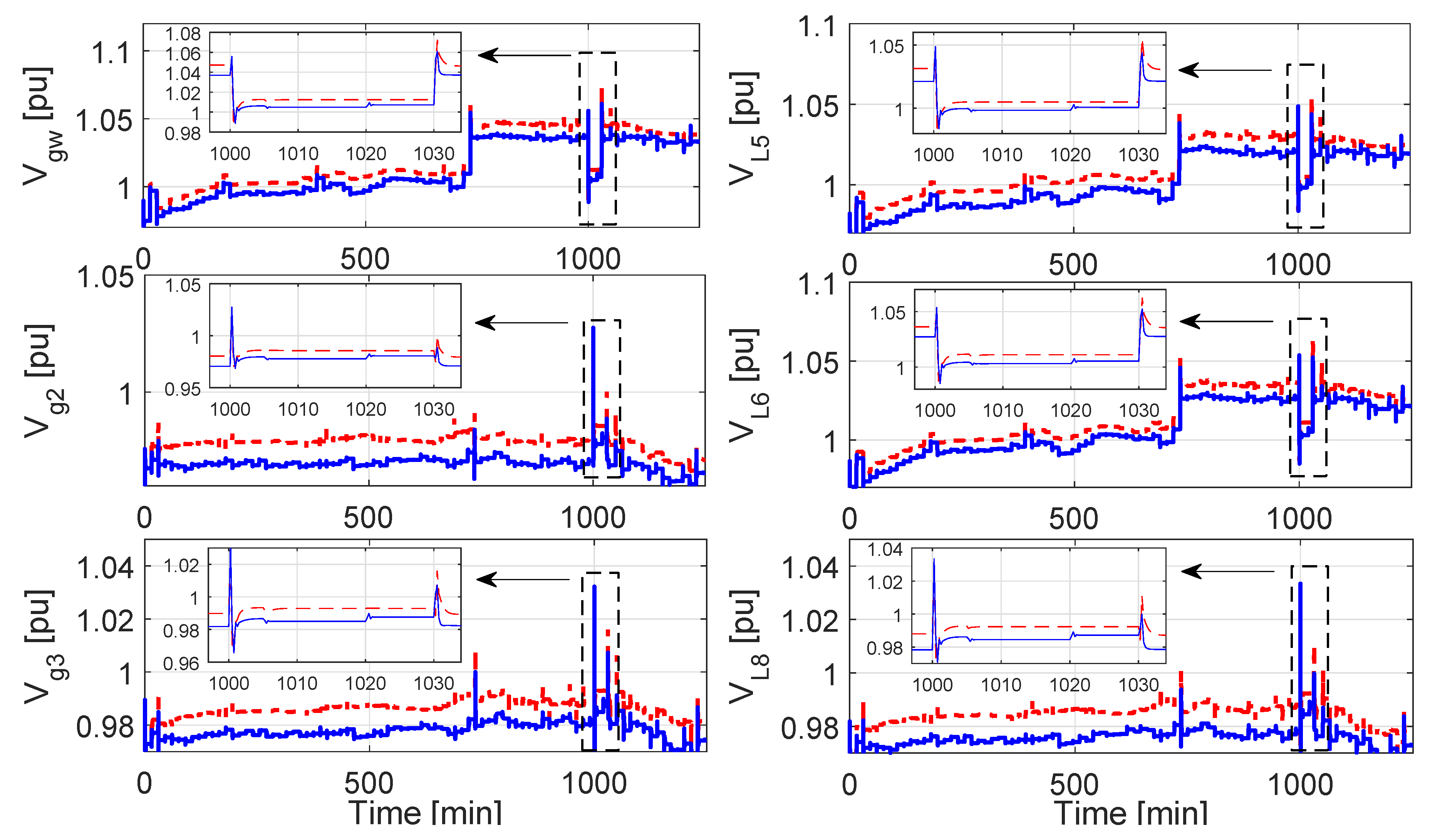
The selection of the IEEE 9-nodes power system benchmark additionally allowed analyzing the behavior of the voltage profile along the simulation. Voltage profile was analyzed because (at the customer level) it is one of the most sensitive variables to the integration of NCES. Moreover, large levels of integration of NCES at the customer level might cause reverse power flows at both over and under voltages. Figure 3 presents the evolution of the voltage profile through the simulation (only the voltage profile under a sudden disconnection of the wind turbine was considered, since similar results were obtained in the case of a load impact). In this figure, the voltage profile with the proposed EMS has a lower value than that of the EMS with perfect predictions. Such a result suggests that less reactive power is flowing trough the lines, which can be traduced in a better use of the industrial network infrastructure and in a reduction of energy costs due to reactive power consumption. Note that once the wind turbine starts to inject power into the grid, the voltage at the point of common coupling raises, as well as the voltage at the load centers. This is consistent with the results reported in the literature about integration of NCES in weak networks such as distribution and industrial ones. However, with the proposed EMS, the transient behavior generated by the injection of wind power is attenuated faster than with the EMS with perfect predictions. Then, (as expected) the proposed EMS provides more robustness to the system as a whole than the EMS with perfect predictions. Such robustness is exhibited in the reduction of power changes in the distribution side, and in a fastest attenuation of the transients produced by the variability of the wind power injections and other disturbances. In fact, the transients associated with the sudden interruption of power supplied from the wind turbine and its corresponding re-connection were better addressed by the system when the proposed EMS was scheduling the local co-generation unit and the power to be imported from the distribution grid. This result is shown in the zoom-in squares of Figure 3.

However, enhancing the robustness of the grid implies an increase in the operating costs, due to a rising in the time of use of the local co-generation unit and the amount of power imported from the grid. From Figure 1, such an increase is more evident during the first 800 min of simulation. In this time-span, the amount of power imported from the distribution grid is slightly higher with the proposed EMS than with the EMS with perfect predictions. The difference in power taken from the grid is traduced in an increment in the cumulative operating costs of $15.2\%$, which is traduced in better dynamic response and use of infrastructure, and in reduction of maximum power fluctuations in the point of common coupling arising from disturbances in the industrial grid. Moreover, the performance of a rolling-horizon-based EMS depends upon the quality of the predictions and hence on the accuracy of the model. Thus, Figure 4 shows a function of the accuracy of the models used to represent the uncertain variables. Indeed, if the model is not accurate enough, the difference between the operating costs with the proposed EMS and the EMS based on the minimization problem of Equation (1) could tend towards zero without the additional benefits provided by the robustness of our proposal.

Furthermore, the computational time required to carry out all the processes involved in the proposed EMS could be an issue. The EMS with perfect predictions only requires the predictions of the uncertain variables. However, for the proposed approach, the time involved in the scenario’s generation and in the solution of the minimization problem of Equation (2) would be significantly larger. However, as Figure 5 shows, the proposed procedure to determine the number of scenarios to be generated, their generation, the computation of the corresponding probability of occurrence, and the solution of the minimization problem of Equation (2) did not significantly increase the computational time. Actually, the mean execution time of the proposed EMS is about 2.4 times the mean execution time of the EMS with perfect predictions. From our point of view, this is a striking difference between the two approaches assessed in this paper, since as previously discussed, the proposed EMS provides several additional benefits in the operation of the grid, by keeping the execution time within reasonable margins (the average execution time was about $0.767$ s, and the largest execution time was 2.5 s). These results were obtained by means of the tic-toc function of Matlab. Moreover, since the computational time is less than 3 s, and the sampling time used to test the performance of the power system with the proposed robust EMS was 15 min (which is a typical sampling time in this kind of EMS), the sampling time could be dramatically reduced to improve the dynamic response of the system [30]. The minimum sample time to implement the proposed EMS will depend of the capabilities of the co-generation unit to follow the changes in the scheduled power.

4. Discussion and Concluding Remarks

Previous works have documented the effectiveness of robust and stochastic programming energy management systems (EMS) approaches to enhance the performance of micro-grids with high penetration of non-conventional energy resources (NCES); in [14,15,25,26], for example, authors report that EMS based in robust and stochastic programming improved their dynamic response (in comparison with deterministic EMS such as the reported in [27]), including the case of unexpected disturbances (e.g., those beyond the expected variability of NCES like load impacts). However, these approaches have been either formulated for micro-grids (both grid connected and off-grid) or have not focused on promoting the self-consumption instead of fostering the power exchange with a main grid (by maximizing the profit in a net-billing/net-metering scheme).

In this paper, we proposed a stochastic-programming-based EMS to promote the self-consumption in NCES applications, in which additional constraints are included to prevent the power injection to the grid as well as terms to avoid as much as possible the energy curtailment of NCES.The expected scenarios are estimated based on the proposed prediction model, which is composed by a deterministic and a stochastic component. The deterministic component consists of a frequency-based model defined by the spectral decomposition of the available historical data set, e.g., the wind power. The stochastic component consists of an ARMA model that attempts to represent the information still present in the residuals of the deterministic model. Both of them are identified off-line using historical data. Such historical data could come from weather predictions, free available databases, or measurements. Here, we used field measurements for model identification.

Once the model is identified, the predictions are carried out taking into consideration current measurements of the variables, e.g., wind power, and its first two statistical moments, namely, the mean and variance. Current measurements are integrated in the historical data used to identify the prediction models; then the mean and variance of each dataset are computed. Based on this information and considering the models previously identified, scenarios are generated. The number of scenarios to be generated is determined by the error between the first two statistical moments of the scenarios and the first two statistical moments of the original time-series. Note that since our approach is stochastic, it is not necessary to perfectly match the predictions with the real values. Indeed, the idea of using a stochastic approach is to adequately represent the uncertainty present in the predictions, so that the EMS can make a scheduling of the generation units robust enough to withstand any sound realization of the uncertain variables.

We also found that the proposed EMS imported slightly higher amounts of power from the main grid than the deterministic EMS with perfect predictions used for comparison purposes. This increase in the power imported from the main grid, combined with a rising in the use of the local co-generation unit considered in the simulations allowed (i) reducing the power changes in the distribution side in case of local disturbances; and (ii) enhancing the dynamic response of the system by reducing the transients produced by the variability of the wind power injections and other disturbances, without making the operation of the grid significantly costly compared to the EMS with perfect predictions. These findings extend those of [15], confirming that despite the increase in the operating costs, stochastic and robust programming based EMS provides additional benefits to the operation of any application of NCES. In this specific case, applications of NCES were oriented to promote the self-consumption in industrial processes.

In addition, the improvements noted in this paper were independent of the type of industrial process or NCES application. Therefore, the results obtained indicate that the benefits gained with the proposed EMS could be extended to a wide range of NCES applications, that in principle focus on self-consumption. Furthermore, our results provide compelling evidence for taking advantage of local generation resources to provide energy to industrial processes, and suggest that the proposed EMS appears to be an effective alternative to integrate NCES in industrial processes without the constraints, often imposed by the distribution system operators, to the injection of energy surpluses to the distribution grid. However, some limitations are worth noting. Although the results confirmed the potentialities of the proposed EMS, more details about the industrial process should be included to better exploit the features of the EMS. Future work should therefore include a better representation of the industrial process and its operational and physical constraints.

Additionally, we intentionally avoided using storage systems such as batteries, which are known to increase the degrees of freedom in the energy management. Here we promoted the integration of non-conventional energy resources by combining with local co-generation. However, this does not imply that the proposed solution cannot be applied in industrial processes with an energy storage system. In this case, an additional term appears in the cost function and additional constraints related with the operating conditions of the energy storage must be added in the formulation. For instance, if a battery storage system is considered, it must be quantified in the cost function and constraints regarding the available energy have to be included in the optimization problem. Such additional costs and constraints can be modeled as in [26].

Although energy storage systems significantly increase the flexibility of an EMS, including them also increases the initial investment costs as well as the operating and maintenance costs. Furthermore, the proposed approach is focused on those countries where power injection in the distribution grid is not completely regularized. In these countries, the adoption of non-conventional energy solutions has an economic barrier that is related with their investment cost. Thus, reducing it by taking advantage of co-generation is a sound alternative to cope with such an economic barrier. The next step of the proposed approach is to include energy storage solutions once an increase in the integration of non-conventional energy resources in industrial processes is evidenced.

References

- Wright, B. A Review of Unit Commitment. Available online: http://blog.narotama.ac.id/wp-content/uploads/2014/12/A-Review-of-Unit-Commitment.pdf (accessed on 8 January 2018).
- Olivares, D.; Canizares, C.; Kazerani, M. A centralized optimal energy management system for microgrids. In Proceedings of the 2011 IEEE Power and Energy Society General Meeting, Detroit, MI, USA, 24–29 July 2011; pp. 1–6. [Google Scholar]
- Hatziargyriou, N.; Contaxis, G.; Matos, M.; Lopes, J.; Kariniotakis, G.; Mayer, D.; Halliday, J.; Dutton, G.; Dokopoulos, P.; Bakirtzis, A.; et al. Energy management and control of island power systems with increased penetration from renewable sources. In Proceedings of the IEEE Power Engineering Society Winter Meeting, New York, NY, USA, 27–31 January 2002; Volume 1, pp. 335–339. [Google Scholar]
- Kueck, J.D.; Staunton, R.H.; Labinov, S.D.; Kirby, B.J. Microgrid Energy Management System; Technical Report; Consortium of Electric Reliability Technology Solutions: Monterey, CA, USA, 2003. [Google Scholar]
- Farret, F.A.; Simoes, M.G. Integration of Alternative Sources of Energy; John Wiley and Sons Inc.: Hoboken, NJ, USA, 2006. [Google Scholar]
- Kroposki, B.; Sen, P.K.; Malmedal, K. Selection of Distribution Feeders for Implementing Distributed Generation and Renewable Energy Applications. IEEE Trans. Ind. Appl. 2013, 49, 2825–2834. [Google Scholar] [CrossRef]
- Chu, K.C.; Kaifuku, K.; Saitou, K. Optimal integration of alternative energy sources in production systems for minimum grid dependency and outage risk. In Proceedings of the 2014 IEEE International Conference on Automation Science and Engineering (CASE), Taipei, Taiwan, 18–22 August 2014; pp. 640–645. [Google Scholar]
- Wang, S.; Huang, G.; Yang, B. An interval-valued fuzzy-stochastic programming approach and its application to municipal solid waste management. Environ. Model. Softw. 2012, 29, 24–36. [Google Scholar] [CrossRef]
- Bertsimas, D.; Litvinov, E.; Sun, X.A.; Zhao, J.; Zheng, T. Adaptive robust optimization for the security constrained unit commitment problem. IEEE Trans. Power Syst. 2013, 28, 52–63. [Google Scholar] [CrossRef]
- Wang, S.; Huang, G. An interval-parameter two-stage stochastic fuzzy program with type-2 membership functions: An application to water resources management. Stoch. Environ. Res. Risk Assess. 2013, 27, 1493–1506. [Google Scholar] [CrossRef]
- Wang, S.; Huang, G. A two-stage mixed-integer fuzzy programming with interval-valued membership functions approach for flood-diversion planning. J. Environ. Manag. 2013, 117, 208–218. [Google Scholar] [CrossRef] [PubMed]
- Nie, X.; Huang, G.; Li, Y.; Liu, L. IFRP: A hybrid interval-parameter fuzzy robust programming approach for waste management planning under uncertainty. J. Environ. Manag. 2007, 84, 1–11. [Google Scholar] [CrossRef] [PubMed]
- Boyd, S.; Vandenberghe, L.; Grant, M. Efficient convex optimization for engineering design. In Proceedings of the IFAC Symposium on Robust Control Design, Rio de Janeiro, Brazil, 14–16 September 1994. [Google Scholar]
- Zhao, B.; Shi, Y.; Dong, X.; Luan, W.; Bornemann, J. Short-Term Operation Scheduling in Renewable-Powered Microgrids: A Duality-Based Approach. IEEE Trans. Sustain. Energy 2014, 5, 209–217. [Google Scholar] [CrossRef]
- Zhang, Y.; Gatsis, N.; Giannakis, G.B. Robust energy management for microgrids with high-penetration renewables. IEEE Trans. Sustain. Energy 2013, 4, 944–953. [Google Scholar] [CrossRef]
- Zhao, C.; Wang, J.; Watson, J.P.; Guan, Y. Multi-Stage Robust Unit Commitment Considering Wind and Demand Response Uncertainties. IEEE Trans. Power Syst. 2013, 28, 2708–2717. [Google Scholar] [CrossRef]
- Yu, Z.; McLaughlin, L.; Jia, L.; Murphy-Hoye, M.; Pratt, A.; Tong, L. Modeling and stochastic control for Home Energy Management. In Proceedings of the 2012 IEEE Power and Energy Society General Meeting, San Diego, CA, USA, 22–26 July 2012; pp. 1–9. [Google Scholar]
- Renewables 2017 Global Status Report. Available online: http://www.ren21.net/gsr-2017/ (accessed on 9 January 2018).
- Fais, B.; Sabio, N.; Strachan, N. The critical role of the industrial sector in reaching long-term emission reduction, energy efficiency and renewable targets. Appl. Energy 2016, 162, 699–712. [Google Scholar] [CrossRef]
- Mao, M.; Jin, P.; Zhao, Y.; Chen, F.; Chang, L. Optimal allocation and economic evaluation for industrial PV microgrid. In Proceedings of the 2013 IEEE Energy Conversion Congress and Exposition, Denver, CO, USA, 15–19 September 2013; pp. 4595–4602. [Google Scholar]
- McManus, M. Environmental consequences of the use of batteries in low carbon systems: The impact of battery production. Appl. Energy 2012, 93, 288–295. [Google Scholar] [CrossRef] [Green Version]
- Boyd, S.; Vandenberghe, L. Convex Optimization; Cambridge University Press: Cambridge, UK, 2004. [Google Scholar]
- Hernandez, L.; Baladron, C.; Aguiar, J.M.; Carro, B.; Sanchez-Esguevillas, A.J.; Lloret, J.; Massana, J. A Survey on Electric Power Demand Forecasting: Future Trends in Smart Grids, Microgrids and Smart Buildings. IEEE Commun. Surv. Tutor. 2014, 16, 1460–1495. [Google Scholar] [CrossRef]
- Ssekulima, E.B.; Anwar, M.B.; Hinai, A.A.; Moursi, M.S.E. Wind speed and solar irradiance forecasting techniques for enhanced renewable energy integration with the grid: A review. IET Renew. Power Gen. 2016, 10, 885–989. [Google Scholar] [CrossRef]
- Valencia, F.; Sáez, D.; Collado, J.; Ávila, F.; Marquez, A.; Espinosa, J.J. Robust energy management system based on interval fuzzy models. IEEE Trans. Control Syst. Technol. 2016, 24, 140–157. [Google Scholar] [CrossRef]
- Valencia, F.; Collado, J.; Sáez, D.; Marín, L.G. Robust Energy Management System for a Microgrid Based on a Fuzzy Prediction Interval Model. IEEE Trans. Smart Grid 2016, 7, 1486–1494. [Google Scholar] [CrossRef]
- Palma-Behnke, R.; Benavides, C.; Lanas, F.; Severino, B.; Reyes, L.; Llanos, J.; Saez, D. A Microgrid Energy Management System Based on the Rolling Horizon Strategy. IEEE Trans. Smart Grid 2013, 4, 996–1006. [Google Scholar] [CrossRef]
- Pizano-Martínez, A.; Fuerte-Esquivel, C.; Zamora-Cárdenas, E.; Segundo Ramírez, J. Conventional Optimal Power Flow Analysis Using the Matlab Optimization Toolbox. In Proceedings of the International ROPEC, Manzanillo, Mexico, 10–12 November 2010. [Google Scholar]
- Sauer, P.W.; Pai, M. Power system dynamics and stability. Urbana 1997, 51, 61801. [Google Scholar]
- Valencia, F.; Marquez, A. An economic robust programing approach for the design of energy management systems. In Power Quality in Future Electrical Power Systems; Energy Engineering; The Institution of Engineering and Technology (IET): Stevenage, UK, 2017; Chapter 11; pp. 359–377. [Google Scholar]
Figure 1.
Power delivered by the wind turbine (red), and total power demand of the industrial process (blue) used in the simulations. After 900 min, the non-conventional energy sources (NCES) provides enough power to satisfy the demand.
Figure 2.
Result obtained from the simulations with both the proposed Energy Management System (solid blue line) and the EMS with perfect predictions of Equation (1) (dashed red line). (a) Power imported from the grid (top) and locally generated (bottom) under a sudden disconnection of the wind turbine at 1000 min; (b) Power imported from the grid (top) and locally generated (bottom) under a load impact at 1000 min.
Figure 3.
Voltages in the main nodes of the power system under unexpected reduction of the wind power. Proposed robust EMS (solid blue line). EMS with perfect prediction (dash red line).
Figure 4.
Evolution of the operating costs during the simulation.
Figure 5.
Computational time of the proposed EMS (blue solid line) and the EMS with perfect predictions (red dashed line).
© 2018 by the authors. Licensee MDPI, Basel, Switzerland. This article is an open access article distributed under the terms and conditions of the Creative Commons Attribution (CC BY) license (http://creativecommons.org/licenses/by/4.0/).
Share and Cite
MDPI and ACS Style
Barrientos, J.; López, J.D.; Valencia, F. A Novel Stochastic-Programming-Based Energy Management System to Promote Self-Consumption in Industrial Processes. Energies 2018, 11, 441. https://doi.org/10.3390/en11020441
AMA Style
Barrientos J, López JD, Valencia F. A Novel Stochastic-Programming-Based Energy Management System to Promote Self-Consumption in Industrial Processes. Energies. 2018; 11(2):441. https://doi.org/10.3390/en11020441
Chicago/Turabian StyleBarrientos, Jorge, José David López, and Felipe Valencia. 2018. "A Novel Stochastic-Programming-Based Energy Management System to Promote Self-Consumption in Industrial Processes" Energies 11, no. 2: 441. https://doi.org/10.3390/en11020441
Note that from the first issue of 2016, this journal uses article numbers instead of page numbers. See further details here.