Nonlinear Modeling and Inferential Multi-Model Predictive Control of a Pulverizing System in a Coal-Fired Power Plant Based on Moving Horizon Estimation

Abstract

Fuel preparation is the control bottleneck in coal-fired power plants due to the unmeasurable nature or inaccurate measurement of key controlled variables. This paper proposes an inferential multi-model predictive control scheme based on moving horizon estimation for the fuel preparation system in coal-fired power plants, i.e., the pulverizing system, aimed at improving control precision of key operating variables that are unmeasurable or inaccurately measured, and improving system tracking performance across a wide operating range. We develop a first principle model of the pulverizing system considering the nonlinear dynamics of primary air, and then employ the genetic algorithm to identify the unknown model parameters. The outputs of the identified first principle model agree well with measured data from a real pulverizing system. Thereafter we derive a moving horizon estimation approach to estimate the desired, but unmeasurable or inaccurately measured, controlled variables. Estimation constraints are explicitly considered to reduce the influence of measurement uncertainty. Finally, nonlinearity of the pulverizing system is analyzed and a multi-model inferential predictive controller is developed using the extended input-output state space model to achieve offset-free performance. Simulation results show that the proposed soft sensor can provide improved estimates than conventional extended Kalman filter, and the proposed inferential control scheme can significantly improve performance of the pulverizing system.

1. Introduction

The pulverizing system is one of the most important auxiliary parts in coal-fired power plants, and has two main functions: to grind crushed coal lumps of several cm in diameter to very fine powder (~50–100 µm in diameter), and sending the pulverized coal into the furnace and provide oxygen for its combustion [1]. The operation performance of the pulverizing system can strongly affect the fuel combustion in the furnace, and thus improving its control performance is of great significance to achieve flexible power plant operation. There are three fundamental control requirements in the pulverizing system.

(1)

Pulverized coal flow into the furnace should rapidly track the power plant fuel demand, allowing power generation to be adjusted in a timely way, as required by power grids.

(2)

The air to coal ratio (the ratio of primary air mass flow to raw coal mass flow) should be kept close to optimal to maintain coal combustion efficiency and reduce generation of nitrogen oxide pollutants [2].

(3)

The coal mill outlet temperature must be controlled within the safe operation region to avoid wet coal conditions and coal firing [3].

However, most power plants are unable to measure pulverized coal flow into the furnace in real-time, which can significantly reduce control precision of the pulverizing system and power plant load [4]. Although hardware sensors, such as digital holography techniques [5], provide some options to solve this problem, they requires very high equipment investment, retrofitting, and maintenance costs, which make their widespread use difficult. The raw coal feed rate and primary air mass flow are also only measured approximately due to measurement technology limitations [6], which introduces many disturbances to the control system and causes fluctuation of the controlled variables.

A practical way to control unmeasurable or inaccurately measured process variables is to apply inferential control schemes, where the desired controlled variables are first estimated by a soft sensor, and subsequently employed as the feedback signal for the controller [7]. Modeling the pulverizing system provides a theoretical foundation to develop soft sensors. Agrawal et al. developed a unified thermal-mechanical model of the pulverizing system that divided coal mill internal regions into four zones and coal particles into ten size groups to consider the fineness of the pulverized coal flow into the furnace [4]; however the model is quite complex and unsuitable for control system design. Niemczyk et al. constructed and validated a dynamic pulverizing system model for different coal mill types under various operating conditions [8], and discussed the influence of classifier speed on pulverized coal flow into the furnace; however many plant details are required in their model, such as the roller breakage rate and flow parameters of the pulverized coal flow. Jin et al. established the dynamic relation between coal mill differential pressure and pulverized coal stored in the mill [9], and Zeng et al. modeled moisture content in pulverized coal by energy balance [10]; however their models ignored the nonlinear dynamics of primary air. Wei et al. developed a multi-segment model that considers coal mill dynamics from startup to shutdown separately [11], however they did not consider the moisture content and grindability of raw coal. In summary, current pulverizing system models are either too simple, too complex, or require many internal plant details, which limit their application for designing soft sensors or control systems. Most previous research has focused on simulation or fault detection of the grinding process, with primary air system dynamics simplified to linear steady-state. In practice, the primary air system is controlled via two air baffles, which have typically nonlinear dynamics. Ignoring these effects will significantly reduce accuracy when the model is used for control system or soft sensor design.

The pulverizing system is a nonlinear multi-variable system with large process inertia and measurement uncertainty, which is difficult for conventional proportional-integral-derivative (PID) controllers to control. Hence, various advanced control techniques have been proposed to improve operational performance. Lu et al. designed a fuzzy PID controller to control outlet temperature [12], however the fuzzy PID cannot handle the large process inertia well. Internal stability and tracking performance of the pulverizing system can be guaranteed with a Lyapunov function, and Fei et al. developed a robust fuzzy tracking control method [13]; however their control scheme cannot achieve the decoupling control of pulverizing system. Cortinovis et al. designed a nonlinear model predictive controller (NMPC) based on a nonlinear pulverizing system model, and updated the model parameters online with an extended Kalman Filter [14]. Although the simulation results show their control strategy is effective, NMPC is generally unable to be solved in real-time. Gao et al. designed a multi-model predictive controller for different operating points, explicitly considering the moisture content of raw coal [6], and developed an optimization control scheme for pulverized coal flow into the furnace; however they did not consider the inaccurate measurements of the key controlled variables. Zeng et al. proposed an economic control method to improve coal combustion efficiency by controlling the moisture content in the pulverized coal to an optimized set point [10]; however they did not discuss the control of pulverized coal flow into the furnace.

Although control problems associated with nonlinearities, coupling effects, and large process inertia have been widely studied for the pulverization system in previous research, few have focused on development of a soft sensor to address issues caused by the fact key controlled variables, i.e., pulverized coal flow into the furnace and primary air mass flowrate, are either unmeasurable or inaccurately measured. The most direct method to estimate desired controlled variables is to solve the model differential equations given measured inputs [4,6,10]. However, this can produce unreliable results. As discussed earlier, raw coal feed rate and primary air mass flow are only measured approximately, and using them directly to estimate pulverized coal flow into the furnace will lead to large errors. Other process measurements, such as mill electric current and outlet temperature, which could reflect the operating status of the grinding process, have not been considered for estimating pulverized coal flow into the furnace.

Considering these issues, this study develops an inferential multi-model predictive control scheme for pulverizing systems. A first principle model of the pulverizing system considering primary air nonlinear dynamics was developed, with model complexity and accuracy balanced by combining physical and empirical relationships. Based on the established model, a soft sensor was derived to estimate desired controlled variables using a moving horizon estimation (MHE) approach, where estimation constraints were explicitly considered to reduce the influence of measurement uncertainty. Finally, the pulverizing system nonlinearity was analyzed, and an inferential multi-model predictive controller designed using the extended input-output state space model to achieve offset-free performance.

The current study has two major contributions:

(1)

A first principle model of the pulverizing system was developed that explicitly considered the nonlinear dynamics of primary air, which is suitable for designing a system controller and soft sensor.

(2)

An inferential multi-model predictive control scheme was established based on MHE that provided improved pulverizing system control precision and tracking performance.

The main content of this paper is organized as follows: Section 2 presents the first principle model of the pulverizing system. Section 3 derives the soft sensor using MHE, and Section 4 discusses the formulation of the inferential multi-model predictive controller. Section 5 presents simulation results, including accuracy validation of the soft sensor and performance validation of the proposed inferential control scheme. Finally, Section 6 concludes the paper.

2. Dynamic Model of the Pulverizing System

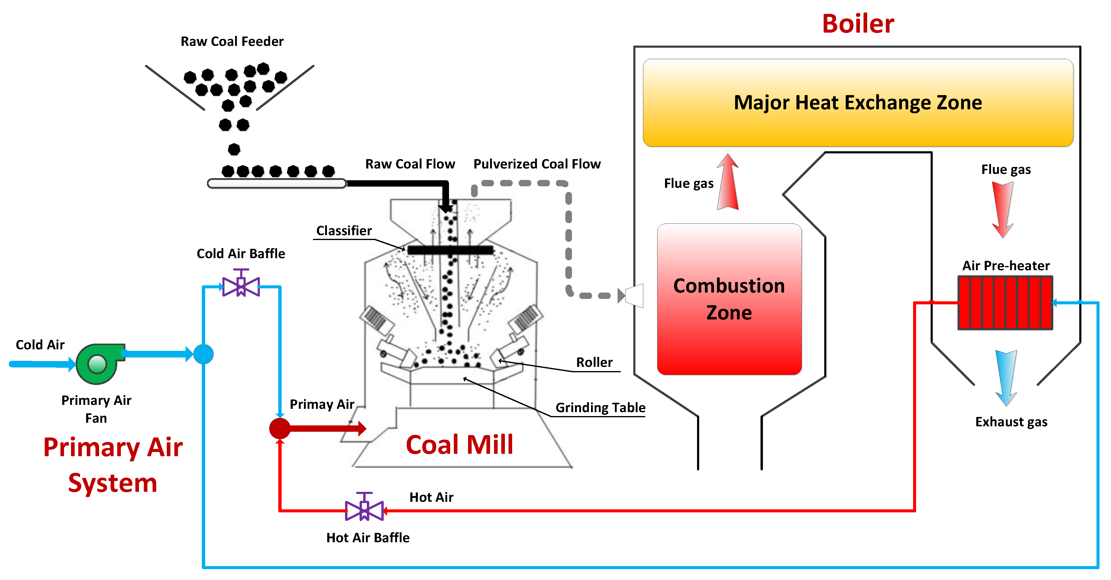
2.1. Pulverizing System Description

Figure 1 shows a typical pulverizing system consisting of coal mill and the primary air systems. In the coal mill, raw coal enters the grinding region from the coal chute and is crushed. Primary air then enters the coal mill through the air ring, drying the pulverized coal and transporting it to the coarse classifier in the upper grinding zone for separation. Suitably pulverized coal is transported by the primary air to the furnace for combustion, whereas unsuitable coal falls back into the coal chute for grinding. The air pre-heater is deployed at the rear of the flue gas tunnel of the boiler, and can heat cold air to ~220 °C. Primary air is generated by mixing cold and hot air, controlled by two air baffles. The primary air fan maintains constant pressure at the entrance of the air baffles. Since the pressure has very fast dynamics, and generally can be well controlled by the primary air fan, the primary air fan has little influence on the pulverizing system operation.

2.2. First Principle Model of the Pulverizing System

The pulverizing system parameter model was established with the following assumptions:

(1)

Raw coal grinding and pulverized coal delivery are separate processes;

(2)

Pulverized coal fineness is neglected, and the coal is categorized into raw and pulverized coal only;

(3)

The classifier operates at its designed rotating speed;

(4)

Primary air is regarded as an ideal gas.

The pulverizing system has 24 unknown parameters to be identified: 8 in the primary air system (S_i, i = 1, 2, …, 8), and 16 in the coal mill system (K_i, i = 1, 2, …, 16).

The dynamics of the primary air system can be described as:

$$q_{air,cold}=S_1{({\mu }_{cold})}^{S_2},$$

(1)

$$q_{air,hot}=S_3{({\mu }_{hot})}^{S_4},$$

(2)

$$S_5\frac{d{t}_{air}}{dt}=\frac{q_{air,cold}}{q_{air,hot}+q_{air,cold}}\cdot t_{cold}+\frac{q_{air,hot}}{q_{air,hot}+q_{air,cold}}\cdot t_{hot}-S_6{t}_{air},$$

(3)

and:

$$S_7\frac{d{q}_{air}}{dt}=q_{air,cold}+q_{air,hot}-S_8{q}_{air},$$

(4)

where $t_{air}$ is the primary air temperature, $q_{air}$ is the primary air mass flow, ${\mu }_{cold}$ is the cold air baffle opening, ${\mu }_{hot}$ is the hot air baffle opening, $t_{cold}$ is the cold air temperature, and $t_{hot}$ is the hot air temperature.

Remark 1.

The air baffle has similar characteristics to valves [15]. Figure 2 shows typical valve inherent flow characteristics, and all of the curves can be well approximated by power functions with different exponents. Thus, we used (1) and (2) to identify air baffle flow characteristics.

The mass balance of raw and pulverized coal is:

$$\frac{d{m}_{raw}}{dt}=q_{raw}-K_1\cdot m_{raw}$$

(5)

and:

$$\frac{d{m}_{pul}}{dt}=K_1\cdot m_{raw}-q_{pul},$$

(6)

where $q_{raw}$ is the mass of raw coal provided by the coal feeder per unit time, $q_{pul}$ is mass flowrate of pulverized coal into the furnace, $m_{raw}$ is the mass of raw coal stored in the mill, and $m_{pul}$ is the pulverized coal stored in the mill.

The primary air blows part of the pulverized coal to the furnace, which is proportional to the differential pressure of primary air ($\Delta p_{air}$) and pulverized coal stored in the mill [6]:

$$q_{pul}\propto \Delta p_{air}\cdot m_{pul},$$

(7)

and from Bernoulli’s equation:

$$\Delta p_{air}=\lambda \cdot {\rho }_{air}\cdot \frac{v_{air}^2}{2g},$$

(8)

where ${\rho }_{air}$ and ${\nu }_{air}$ are the primary air density and flow speed, and λ is the flow resistance. Since the primary air is assumed to be an ideal gas, ${\rho }_{air}$ is proportional to the air temperature air, hence:

$$q_{pul}=K_2(273.15+t_{air})\cdot q_{air}^2{m}_{pul}.$$

(9)

Using conservation laws, the total energy balance in the mill is:

$$\Delta E_{mill}=Q_{in}-Q_{out},$$

(10)

$$Q_{in}=Q_{air,in}+Q_{coal,in}+Q_I,$$

(11)

and:

$$Q_{out}=Q_{air,out}+Q_{coal,out}+Q_{vapor}+Q_{loss},$$

(12)

where $\Delta E_{mill}$ is the increment of inner energy; $Q_{air,in}$ and $Q_{coal,in}$ are the energy brought to the mill by the primary air and raw coal, respectively; $Q_I$ is the heat generated by the mill electric current; $Q_{air,out}$ and $Q_{coal,out}$ are the energy removed by primary air and pulverized coal flow to the furnace, respectively; $Q_{vapor}$ is the heat loss from evaporation; and $Q_{loss}$ is the heat loss to the environment.

Various terms in (10), (11) and (12) can be expressed as follows:

$$\begin{array}{c}\Delta E_{mill}=C_{mill}\frac{d(M_{mill}{t}_m)}{dt}=C_{mill}{t}_m\frac{d{M}_{mill}}{dt}+C_{mill}{M}_{mill}\frac{d{t}_m}{dt}\\ =K_3{t}_m(\frac{d{m}_{raw}}{dt}+\frac{d{m}_{pul}}{dt})+K_3(K_4+m_{raw}+m_{pul})\frac{d{t}_m}{dt}\end{array},$$

(13)

$$Q_{air,in}=C_a{q}_{air}{t}_{air},$$

(14)

$$Q_{coal,in}=K_5{q}_{raw}{t}_{envi},$$

(15)

$$Q_I=K_{6}I,$$

(16)

$$Q_{air,out}=C_a{q}_{air}{t}_m,$$

(17)

$$Q_{coal,out}=K_7{q}_{pul}{t}_m,$$

(18)

$$Q_{vapor}=K_8{q}_{water},$$

(19)

and:

$$Q_{loss}=K_9(t_m-t_{envi}),$$

(20)

where $t_{envi}$ is the environment temperature, $I$ is the coal mill electric current, $t_m$ is the outlet temperature, $q_{water}$ is the mass flow rate of evaporated water, $C_a$ is the heat capacity of air, $C_{mill}$ is the heat capacity of the pulverizing system, and $M_{mill}$ is the total mass of pulverizing system.

Evaporation mainly occurs inside the coal mill, hence moisture evaporation speed depends on the raw and pulverized coal stored in the coal mill, and is also exponentially related to the air mass flow [10]. Thus:

$$q_{water}=\theta (m_{raw}+m_{pul})t_m(1-\exp (-\frac{q_{air}}{K_{10}})),$$

(21)

where $\theta$ is the moisture content in raw coal.

Mill differential pressure, $\Delta p_{mill}$, depends on the amount of pulverized coal carried by the primary air and flow resistance, which is assumed to be linearly related to the raw coal stored in the mill [4]. Thus:

$$\Delta p_{mill}=(K_{11}+K_{12}{m}_c)q_{air}^2+K_{13}{q}_{pul}.$$

(22)

The pulverizing system electric current is determined by the raw and pulverized coal stored in the mill, and the no-load current, $K_{16}$:

$$I=K_{14}\cdot \eta \cdot m_{raw}+K_{15}{m}_{pul}+K_{16},$$

(23)

where $\eta$ is the grindability of raw coal.

Thus, the model has six measurable inputs, $q_{raw}$, ${\mu }_{cold}$, ${\mu }_{hot}$, $t_{envi}$, $t_{cold}$, $t_{hot}$; two unmeasurable inputs, $\theta$, $\eta$; five model states, $t_{air}$, $q_{air}$, $m_{raw}$, $m_{pul}$, $t_m$; and five measurable outputs, $t_{air}$, $q_{air}$, $I$, $\Delta p_{mill}$, $t_m$. The desired controlled variables are $q_{pul}$, $q_{air}$, and $t_m$ and the manipulated variables are $q_{raw}$, ${\mu }_{cold}$, and ${\mu }_{hot}$, i.e., a three input, three output control system.

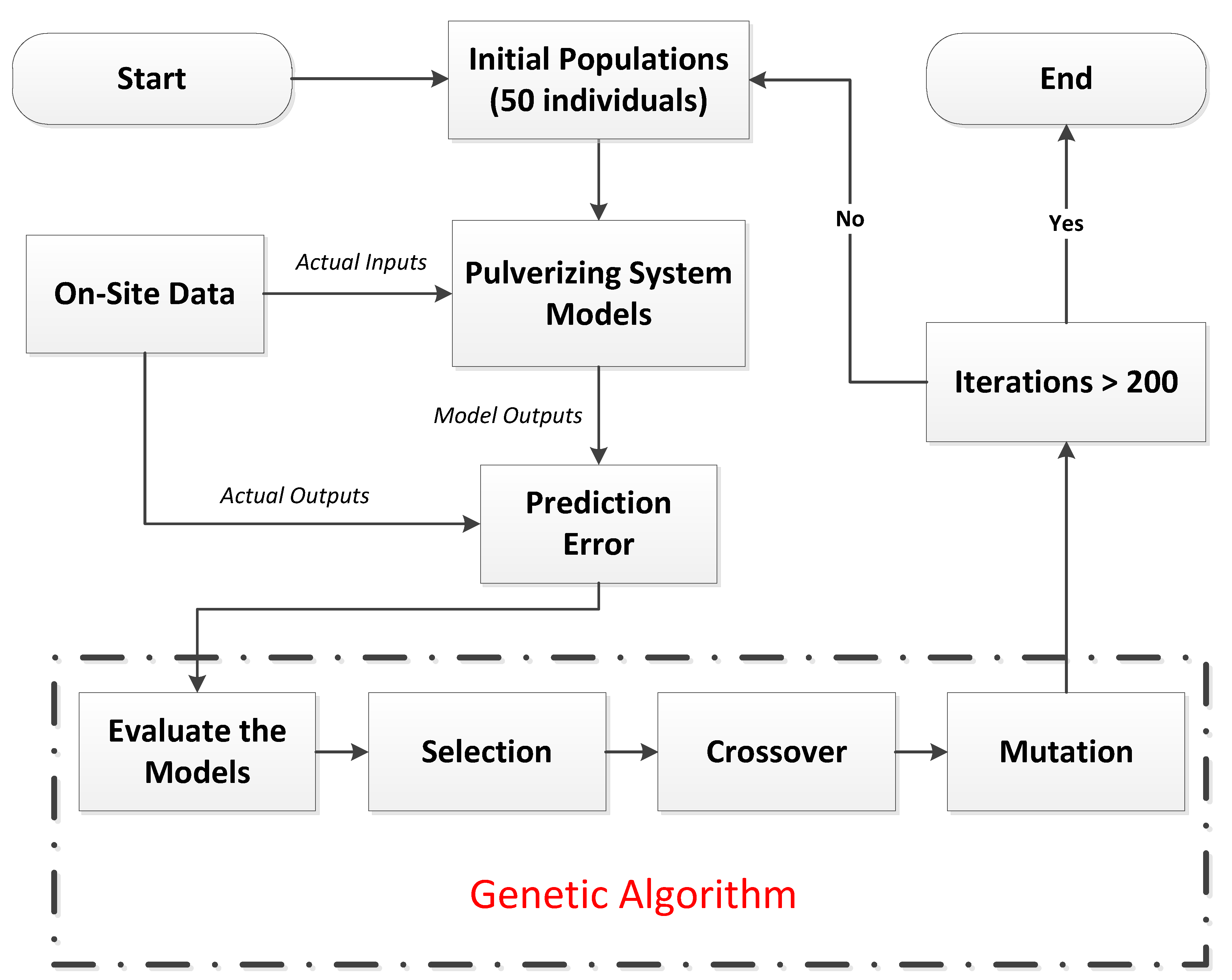
2.3. Parameter Identification

The data set to identify the unknown parameters was collected from a historical database of a 660 MW power plant in China. The output prediction error was employed to evaluate the model accuracy:

$$E({\left\{S_i\right\}}_{i=1,2,\dots ,8},{\left\{K_j\right\}}_{j=1,2,\dots ,17})={\displaystyle \sum _{t=1}^N\left\{\begin{array}{l}{w}_1\Vert \frac{{\widehat{q}}_{air}(t)-q_{air}(t)}{q_{air}(t)}\Vert +w_2\Vert \frac{{\widehat{t}}_{air}(t)-t_{air}(t)}{t_{air}(t)}\Vert +w_3\Vert \frac{\widehat{I}(t)-I(t)}{I(t)}\Vert \\ +w_4\Vert \frac{\Delta {\widehat{p}}_{mill}(t)-\Delta p_{mill}(t)}{\Delta p_{mill}(t)}\Vert +w_5\Vert \frac{{\widehat{t}}_m(t)-t_m(t)}{t_m(t)}\Vert \end{array}\right\}},$$

(24)

where $N$ is number of data points; $q_{air}(i)$, $t_{air}(i)$, $I(i)$, $\Delta p_{mill}(i)$, and $t_m(i)$ are the ith measured outputs; ${\widehat{q}}_{air}(i)$, ${\widehat{t}}_{air}(i)$, $\widehat{I}(i)$, $\Delta {\widehat{p}}_{mill}(i)$, and ${\widehat{t}}_m(i)$ are the ith model outputs; and $w_1$, $w_2$, $w_3$, $w_4$ and $w_5$ are the output weights. A genetic algorithm (GA) was used to minimize (24) and obtain optimal unknown parameters. Compared with more recently developed particle swarm optimization (PSO), GA has a better chance of finding a more qualified solution, since the mutation operation can make the population cluster around several “good” solutions instead of one “good” solution [17]. Moreover it has been demonstrated that GA is robust in the parameter identification problem and can achieve good results [18,19]. GA processes are well explained elsewhere [20], and we present the identification process of GA in Figure 3.

Table 1. Genetic algorithm tuning parameters.

Population Size	Probability of Mutation	Probability of Crossover	Termination Iterations	Generation Gap	${\mathit{w}}_1$	${\mathit{w}}_2$	${\mathit{w}}_3$	${\mathit{w}}_4$	${\mathit{w}}_5$
50	0.3	0.9	200	0.8	2	1	1	1.5	1

and

Table 2. Final optimal model parameters.

Parameter	S1	S2	S3	S4	S5	S6	S7	S8
Value	0.70	0.66	0.75	0.77	150.1	1.06	22.5	1.08
Parameter	K1	K2	K3	K4	K5	K6	K7	K8
Value	0.053	1.47 × 10−6	1423	10,530	1309	2398	1306	5893
Parameter	K9	K10	K11	K12	K13	K14	K15	K16
Value	7037	95	5.29	0.0095	10.26	0.114	0.0292	19.11

show the GA tuning parameters and final optimal parameters, respectively. The tuning parameters are set based on the simulation parameters proposed in [21].

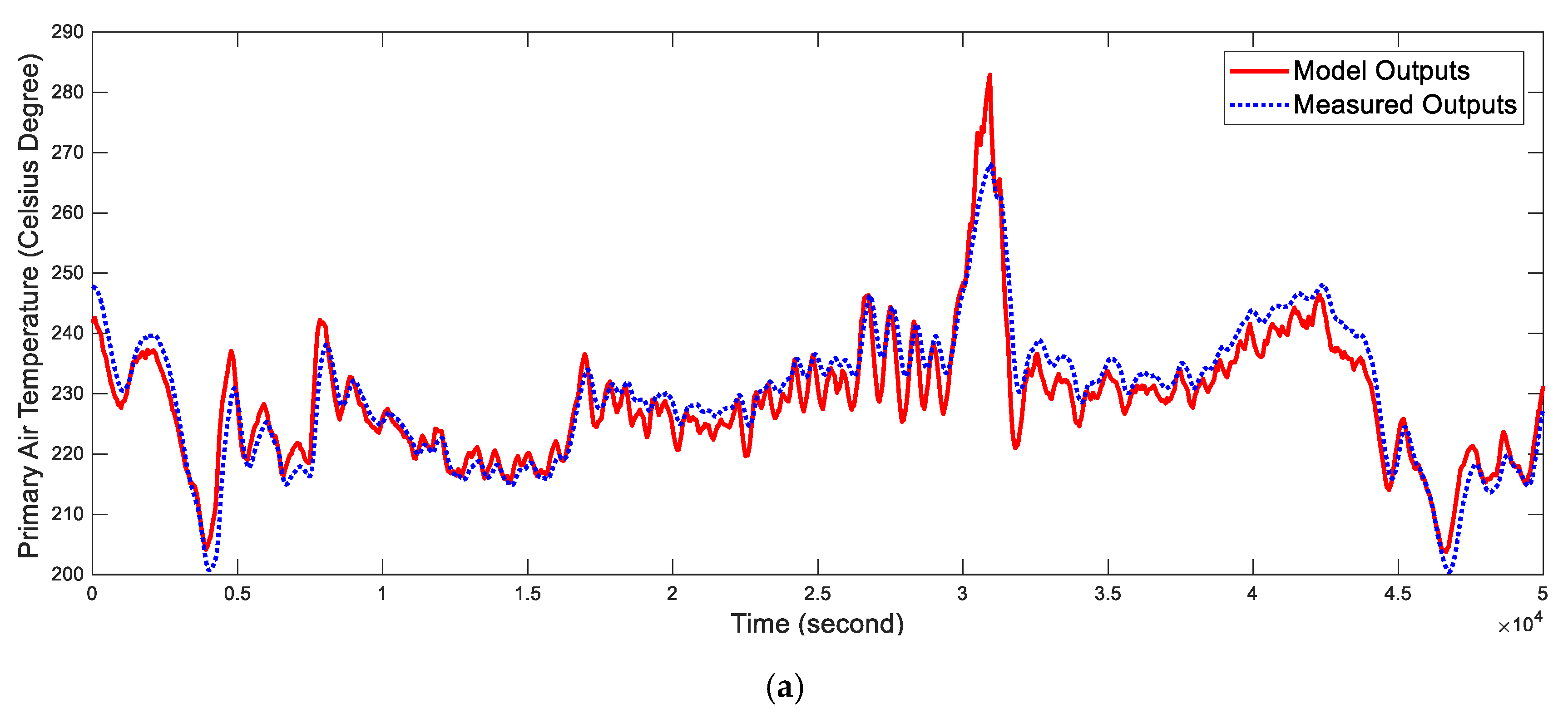
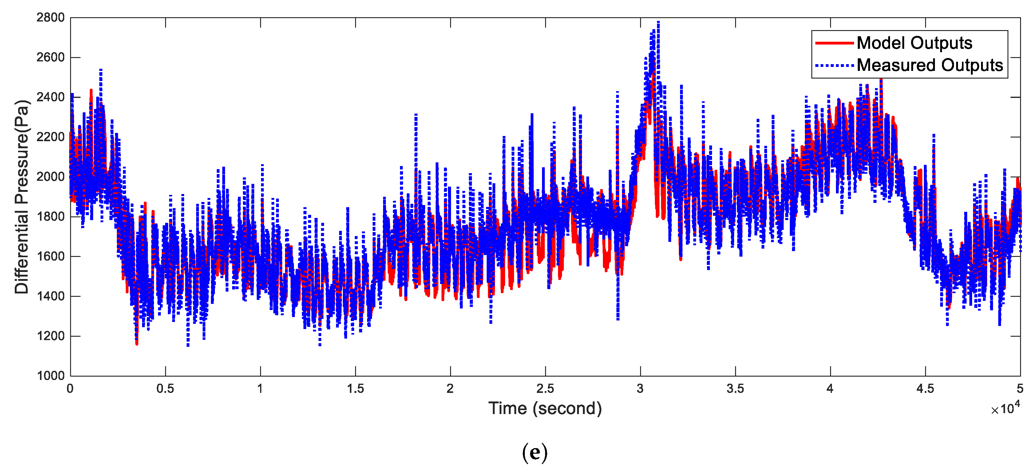
2.4. Model Validation

The proposed model derived in Section 2.3 was validated using a different historical data set where the pulverizing system had a wide operating range (47.03–90.97% load rate), as shown in Figure 4. The real process trends and time constant were well captured by the proposed model. Thus, the model can be employed as the simulation platform for design of the soft sensor and control system.

Table 3. Cumulative relative fitting error.

Primary Air Temperature	Primary Air Mass Flowrate	Electric Current	Outlet Temperature	Differential Pressure
664	1806	852	799	995

shows the cumulative relative fitting error for the five outputs, defined as:

$${\displaystyle \sum _{i=1}^N\left|\frac{y_{\mathrm{model}}^i-y_{real}^i}{y_{real}^i}\right|},$$

(25)

where $N$ is the number of data samples, and $y_{\mathrm{model}}^i$ and $y_{real}^i$ are the model output and process measurement, respectively. The primary air temperature is accurately predicted, whereas the primary air mass flowrate has significantly higher fitting error than other outputs due to the primary air mass flowrate being inaccurately measured in the real plant, as discussed above, and we cannot improve this prediction accuracy by adjusting the model parameters. However, the primary air temperature is accurately measured and the model shows high prediction accuracy.

3. Formulation of the Soft Sensor

The soft sensor to estimating the desired controlled variables was developed using MHE. We first derived the general MHE problem for the pulverizing system, and then discuss updating the arrival cost.

Artificial neural networks have been employed to develop soft sensors for many industrial processes to control unmeasurable variables [22,23,24,25,26]. Although such soft sensors can exhibit high fitting precision on the test data sets, they cannot explain process mechanisms, and hence can lack of robustness in the presence of process uncertainty.

Therefore, we developed the soft sensor using MHE. Moving horizon estimation is a model based optimization method to estimate the states and unknown parameters online and was originally derived as an approximation for the full-information maximum likelihood estimator (FIE) to avoid issues with FIE dimensionality [27]. Similar to model predictive control, MHE solves a finite horizon optimization problem dynamically at each sample time. Hence, the latest measurements available are employed to calculate current estimates. An important advantage of MHE over other soft sensor types is that the estimate constraints can be explicitly considered. Therefore, we can set the operating variable constraints based on prior knowledge of the pulverizing system to improve estimation accuracy.

The pulverizing system model can be expressed as:

$$\{\begin{array}{l}\frac{dx}{dt}=f(x,u,p)\\ y=h(x,u,p)\end{array},$$

(26)

where:

$$x={\left[\begin{array}{ccc}\begin{array}{cc}\begin{array}{cc}{t}_{air}& q_{air}\end{array}& m_{raw}\end{array}& m_{pul}& t_m\end{array}\right]}^T,$$

(27)

$$p={\left[\begin{array}{cc}\theta & \eta \end{array}\right]}^T,$$

(28)

$$u={\left[\begin{array}{cccccc}{\mu }_{hot}& {\mu }_{cold}& q_{raw}& t_{envi}& t_{cold}& t_{hot}\end{array}\right]}^T,$$

(29)

$$y={\left[\begin{array}{ccc}\begin{array}{cc}\begin{array}{cc}{t}_{air}& q_{air}\end{array}& I\end{array}& \Delta p_{mill}& t_m\end{array}\right]}^T,$$

(30)

$$f(x,u,p)=\left[\begin{array}{c}(\frac{S_1{({\mu }_{cold})}^{S_2}}{S_3{({\mu }_{hot})}^{S_4}+S_1{({\mu }_{cold})}^{S_2}}\cdot t_{cold}+\frac{S_3{({\mu }_{hot})}^{S_4}}{S_3{({\mu }_{hot})}^{S_4}+S_1{({\mu }_{cold})}^{S_2}}\cdot t_{hot}-S_6{t}_{air})/S_5\\ (S_1{({\mu }_{cold})}^{S_2}+S_3{({\mu }_{hot})}^{S_4}-S_8{q}_{air})/S_7\\ q_{raw}-K_1\cdot m_{raw}\\ K_1\cdot m_{raw}-K_2(273.15+t_{air})\cdot q_{air}^2{m}_{pul}\\ \frac{(Q_{in}-Q_{out})-K_3{t}_m(q_{raw}-K_2(273.15+t_{air})\cdot q_{air}^2{m}_{pul})}{K_3(K_4+m_{raw}+m_{pul})}\end{array}\right],$$

(31)

$$Q_{in}=C_a{q}_{air}{t}_{air}+K_5{q}_{raw}{t}_{envi}+K_{6}I,$$

(32)

$$Q_{out}=C_a{q}_{air}{t}_m+K_7{K}_2(273.15+t_{air})\cdot q_{air}^2{m}_{pul}{t}_m+K_8\theta (m_{raw}+m_{pul})t_m(1-e^{-\frac{q_{air}}{K_{10}}})+K_9(t_m-t_{envi}),$$

(33)

and:

$$h(x,u,p)=\left[\begin{array}{c}{t}_{air}\\ q_{air}\\ K_{14}\cdot \eta \cdot m_{raw}+K_{15}{m}_{pul}+K_{16}\\ (K_{11}+K_{12}{m}_c)q_{air}^2+K_{13}{q}_{pul}\\ t_m\end{array}\right].$$

(34)

Then the MHE soft sensor is formulated as a nonlinear least squares optimization problem:

$$\underset{\begin{array}{l}{\widehat{x}}_{k-N+1},\dots ,{\widehat{x}}_k\\ {\widehat{p}}_{k-N+1},\dots ,{\widehat{p}}_k\end{array}}{\min }({\Vert \begin{array}{l}{\widehat{x}}_{k-N+1}-{\overline{x}}_L\\ {\widehat{p}}_{k-N+1}-{\overline{p}}_L\end{array}\Vert }_{P_L}^2+{{\displaystyle \sum _{i=k-N+1}^{k-1}\Vert \begin{array}{c}{\widehat{x}}_{i+1}-\varphi ({\widehat{x}}_i,{\widehat{p}}_i,u_i)\\ {\widehat{p}}_{i+1}-{\widehat{p}}_i\end{array}\Vert }}_W^2+{\displaystyle \sum _{i=k-N+1}^k{\Vert y_i-h({\widehat{x}}_i,{\widehat{p}}_i,u_i)\Vert }_V^2}),$$

(35)

where:

$$\varphi ({\widehat{x}}_i,{\widehat{p}}_i,u_i)={\displaystyle {\int }_0^{T}f({\widehat{x}}_i,{\widehat{p}}_i,u_i)dt};$$

(36)

k represents the present time instance; N is the estimation horizon; T is the sampling time; ${\widehat{x}}_{k-N+1},\dots ,{\widehat{x}}_k$ are the state estimates from time k − N+1 to k; ${\widehat{p}}_{k-N+1},\dots ,{\widehat{p}}_k$ are the parameter estimates from time k − N+1 to k; $y_i$ is the measured outputs at time i; $P_L$, V, and W are constant positive definite weighting matrixes; and ${\overline{x}}_L$ and ${\overline{p}}_L$ are constant scalars representing the influence from past measurements. The first term in the cost function (35) is typically called the arrival cost, and is important for MHE stability [28]. ${\overline{x}}_L$, ${\overline{p}}_L$, and $P_L$ are updated when the MHE calculates a new estimate.

The analytical solution for $\varphi ({\widehat{x}}_i,{\widehat{p}}_i,u_i)$ is difficult to find, and we approximate it using forward difference:

$$\varphi ({\widehat{x}}_i,{\widehat{p}}_i,u_i)\approx {\widehat{x}}_i+T\cdot f({\widehat{x}}_i,{\widehat{p}}_i,u_i),$$

(37)

where T should be as small as possible to avoid large approximation error, or it may reduce estimation precision and possibly make the soft sensor unstable. However, since the pulverizing system has large inertia, $f({\widehat{x}}_i,{\widehat{p}}_i,u_i)$ cannot change sharply during the sampling interval, hence (37) will not cause significant approximation error.

Conventionally, ${\overline{x}}_L$, ${\overline{p}}_L$ and $P_L$ are updated using the Kalman filter. However, this introduces large errors for nonlinear systems in the approximation of the full information estimator, which necessitates a large estimation horizon, and increases the online computational burden [29]. Considering this problem, we propose an efficient arrival cost update, based on Kuhl et al. [30]. Arrival cost updating was derived for the discretized pulverizing system model as follows.

The ideal arrival cost can be expressed as:

$$C(x_L,p_L)=\underset{x_{L-1},p_{L-1}}{\min }({\Vert \begin{array}{l}{x}_{L-1}-{\overline{x}}_{L-1}\\ p_{L-1}-{\overline{p}}_{L-1}\end{array}\Vert }_{P_{L-1}}^2+{\Vert y-h(x_{L-1},p_{L-1})\Vert }_V^2+{\Vert \begin{array}{c}{x}_L-\varphi (x_{L-1},p_{L-1})\\ p_L-p_{L-1}\end{array}\Vert }_W^2),$$

(38)

where ${\overline{x}}_{L-1}$ and ${\overline{p}}_{L-1}$ are the states and parameters in the arrival cost term at the previous sampling time. To approximate $C(x_L,p_L)$ using a linear quadratic expression, nonlinear mappings $f(x_{L-1},p_{L-1})$ and $h(x_{L-1},p_{L-1})$ are approximated using Taylor expansion:

$$f(x_{L-1},p_{L-1})\approx f(x^{\ast },p^{\ast })+f_x\cdot (x_{L-1}-x^{\ast })+f_p\cdot (p_{L-1}-p^{\ast }),$$

(39)

and:

$$h(x_{L-1},p_{L-1})\approx h(x^{\ast },p^{\ast })+h_x\cdot (x_{L-1}-x^{\ast })+h_p\cdot (p_{L-1}-p^{\ast }),$$

(40)

where:

$$f_x={\frac{\partial f(x,p)}{\partial x}|}_{x_{L-1}=x^{\ast },p_{L-1}=p^{\ast }},$$

(41)

$$f_p={\frac{\partial f(x,p)}{\partial p}|}_{x_{L-1}=x^{\ast },p_{L-1}=p^{\ast }},$$

(42)

$$h_x={\frac{\partial h(x,p)}{\partial x}|}_{x_{L-1}=x^{\ast },p_{L-1}=p^{\ast }},$$

(43)

$$h_p={\frac{\partial f(x,p)}{\partial p}|}_{x_{L-1}=x^{\ast },p_{L-1}=p^{\ast }},$$

(44)

and $x^{\ast }$ and $p^{\ast }$ are the best available estimate at time k − N. Then:

$$\varphi (x_{L-1},p_{L-1})\approx x_{L-1}+T\cdot f(x_{L-1},p_{L-1}).$$

(45)

Substituting (39), (40), and (45) into (38):

$$C(x_L,p_L)\approx \underset{X_{L-1}}{\min }{\Vert A\left[\begin{array}{l}{X}_{L-1}\\ X_L\end{array}\right]-b\Vert }_2^2,$$

(46)

where:

$$A=\left[\begin{array}{cc}-V{h}_x|-V{h}_p& O\\ -W\left[\begin{array}{cc}I+T\cdot f_x& T\cdot f_p\\ O& I\end{array}\right]& W\\ P_{L-1}& O\end{array}\right],$$

(47)

$$b=\left[\begin{array}{c}V(f(x^{\ast },p^{\ast })-f_x\cdot x^{\ast }-f_p\cdot p^{\ast }-y)\\ W\left[\begin{array}{c}h(x^{\ast },p^{\ast })-h_x\cdot x^{\ast }-h_p\cdot p^{\ast }\\ O\end{array}\right]\\ P_{L-1}\left[\begin{array}{l}{\overline{x}}_{L-1}\\ {\overline{p}}_{L-1}\end{array}\right]\end{array}\right],$$

(48)

$$X_L=\left[\begin{array}{l}{x}_L\\ p_L\end{array}\right],$$

(49)

$$X_{L-1}=\left[\begin{array}{l}{x}_{L-1}\\ p_{L-1}\end{array}\right],$$

(50)

and O and I are zero and unit matrices, respectively, with appropriate dimensions.

Equation (46) can be transformed using QR factorization of $A$ to:

$$C(x_L,p_L)\approx \underset{X_{L-1}}{\min }{\Vert \left[\begin{array}{ccc}{Q}_1& Q_2& Q_3\end{array}\right]\left[\begin{array}{cc}{R}_1& R_{12}\\ O& R_2\\ O& O\end{array}\right]\left[\begin{array}{l}{X}_L\\ X_{L-1}\end{array}\right]-b\Vert }_2^2,$$

(51)

which has the analytic solution:

$$C(x_L,p_L)\approx {\Vert Q_3\cdot b\Vert }_2^2+{\Vert Q_2\cdot b+R_2\left[\begin{array}{l}{x}_L\\ p_L\end{array}\right]\Vert }_2^2,$$

(52)

where:

$$A=\left[\begin{array}{ccc}{Q}_1& Q_2& Q_3\end{array}\right]\left[\begin{array}{cc}{R}_1& R_{12}\\ O& R_2\\ O& O\end{array}\right],$$

(53)

$$P_L=R_2,$$

(54)

$$\left[\begin{array}{l}{\overline{x}}_L\\ {\overline{p}}_L\end{array}\right]=R_2^{-1}\cdot Q_2\cdot b,$$

(55)

and ${\overline{x}}_L$, ${\overline{p}}_L$ and $P_L$ are employed to update the MHE arrival cost.

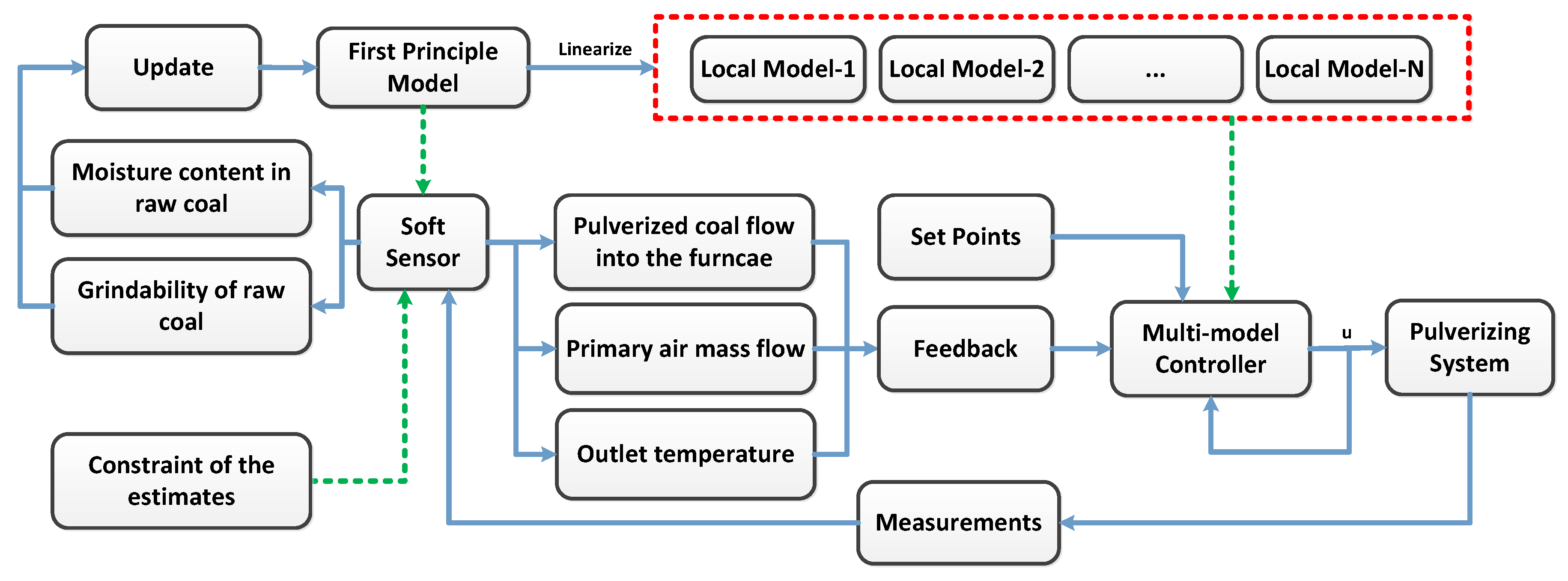
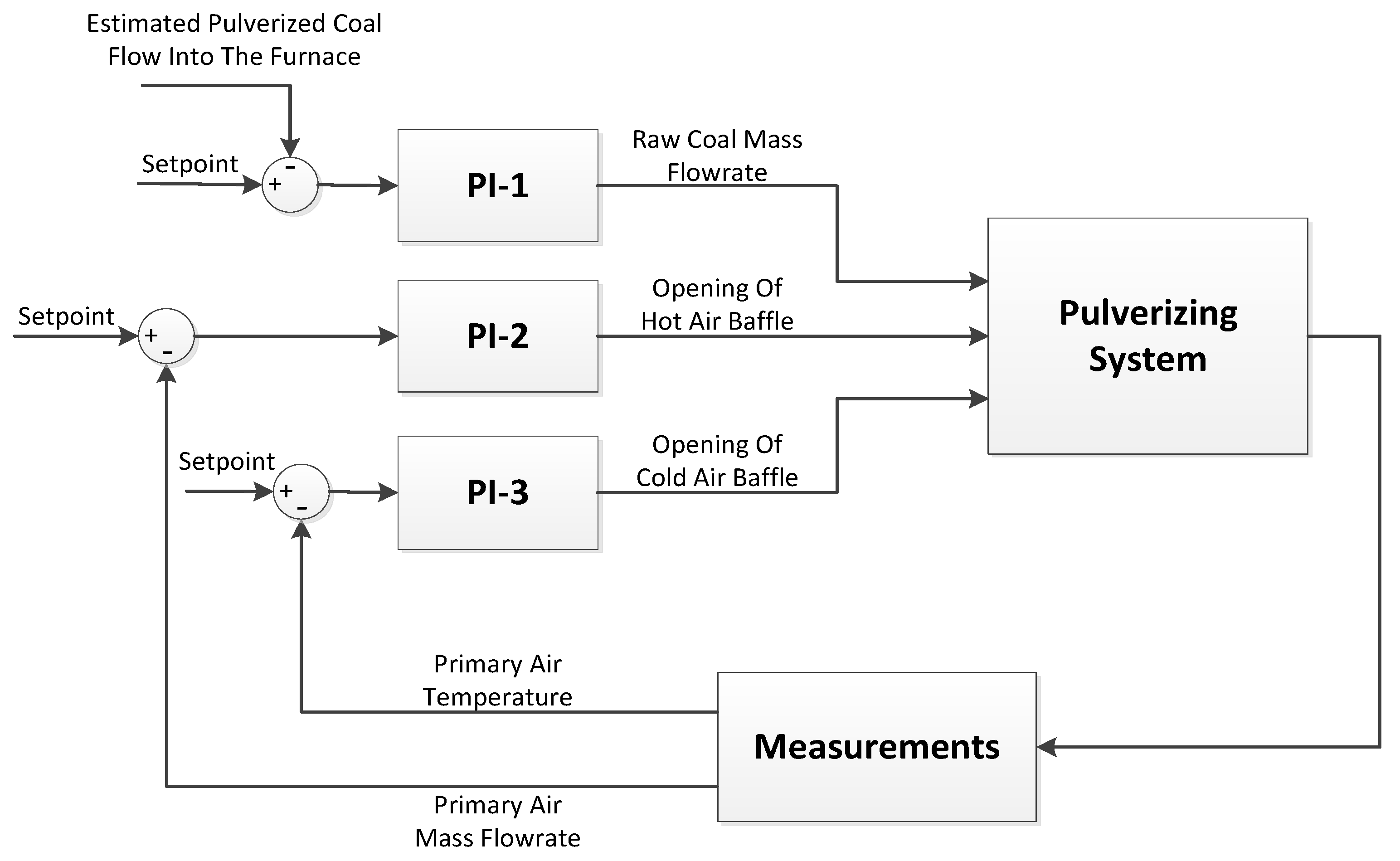
4. Inferential Multi-Model Predictive Controller Design

Nonlinearity of the pulverizing system was analyzed to select proper local models for the multi-model controller, then the predictive controller was designed based on an extended input-output state space model to achieve offset-free performance in the presence of modeling error and unknown disturbances. Figure 5 shows an overall view of the inferential control system.

The soft sensor can not only estimate desired controlled variables but can also detect a change of raw coal. Since different raw coal types have different grindability and moisture content, pulverizing system outputs can change significant when the power plant uses a new raw coal type. Therefore, the soft sensor can be used to update model parameters online.

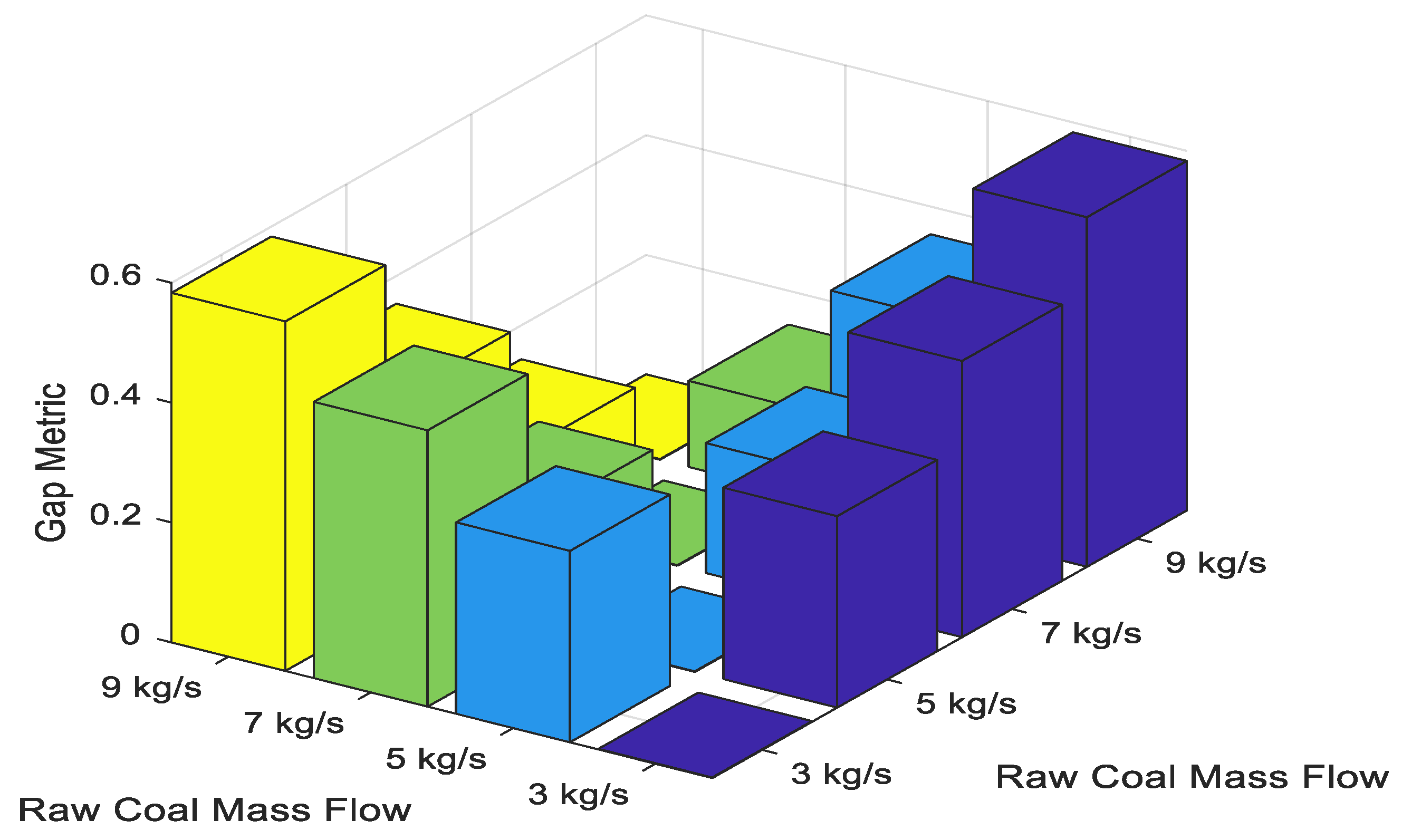
4.1. Nonlinearity Analysis

The basic control task for the pulverizing system is to track power plant coal demand. Hence raw coal feed rate was selected as the scheduling variable to analyze process nonlinearity. In practice, the setpoint of primary air mass flow is set according to the desired air to coal ratio, and is proportional to the raw coal feed rate. There is also a lower limit on primary air mass flow, to avoid coal jamming, and in this case the lower limit = 10 kg/s.

Table 4. Selected operating points.

Raw Coal Feed Rate (kg/s)	Primary Air Mass Flow (kg/s)	Primary Air Temperature (K)	Cold Air Baffle Position (%)	Hot Air Baffle Position (%)	Outlet Temperature (°C)	Mill Electric Current (A)	Mill Differential Pressure (kPa)
3	10.0	195.6	10.7	16.5	70	26.77	0.5995
5	12.5	218.0	9.3	26.2	70	31.10	0.9646
7	17.5	224.2	14.3	46.9	70	35.00	1.9944
9	22.5	235.1	16.6	74.1	70	39.06	3.5074

shows the selected operating points.

Local linear models at typical operating points can be obtained by linearizing the first principle model of the pulverizing system. Then the gap metric was employed to quantitatively measure nonlinearity between local models. The gap metric between two local linear systems $P_1$ and $P_2$ is defined as [31]:

$$\delta (P_1,P_2)=\max \{\underset{Q\in H_{\infty }}{\inf }{\Vert \left[\begin{array}{l}{M}_1\\ N_1\end{array}\right]-\left[\begin{array}{l}{M}_2\\ N_2\end{array}\right]Q\Vert }_{\infty },\underset{Q\in H_{\infty }}{\inf }{\Vert \left[\begin{array}{l}{M}_2\\ N_2\end{array}\right]-\left[\begin{array}{l}{M}_1\\ N_1\end{array}\right]Q\Vert }_{\infty }\},$$

(56)

where $P_1=N_1{M}_1^{-1}$ and $P_2=N_2{M}_2^{-1}$ are the normalized right coprime factorization on $P_1$ and $P_2$, respectively.

If the $\delta (P_1,P_2)\approx 1$, dynamic behavior between the local linear models is significantly different and process nonlinearity is strong between the two operating points. In contrast, if the $\delta (P_1,P_2)\approx 0$, dynamic behavior between the two local models is similar, and process nonlinearity is weak. Figure 6 shows the gap metric between all the local models.

The gap metric is approximately linear with local linear model distance, i.e., the difference of the raw coal feed rate. Therefore, we divided the operating range uniformly by selecting local models with 5 and 9 kg/s raw coal feed rate and employed the selected local models for controller design. When $\delta (P_1,P_2)<0.3$ between any operating point and one of the selected operating points, nonlinearity within the local controller working range is not strong. The proposed division of the operating range can satisfy this condition. Although we can select all four models to set up the multi-model controller, this will lead to heavy online computation overhead, for insignificant improvement in control performance.

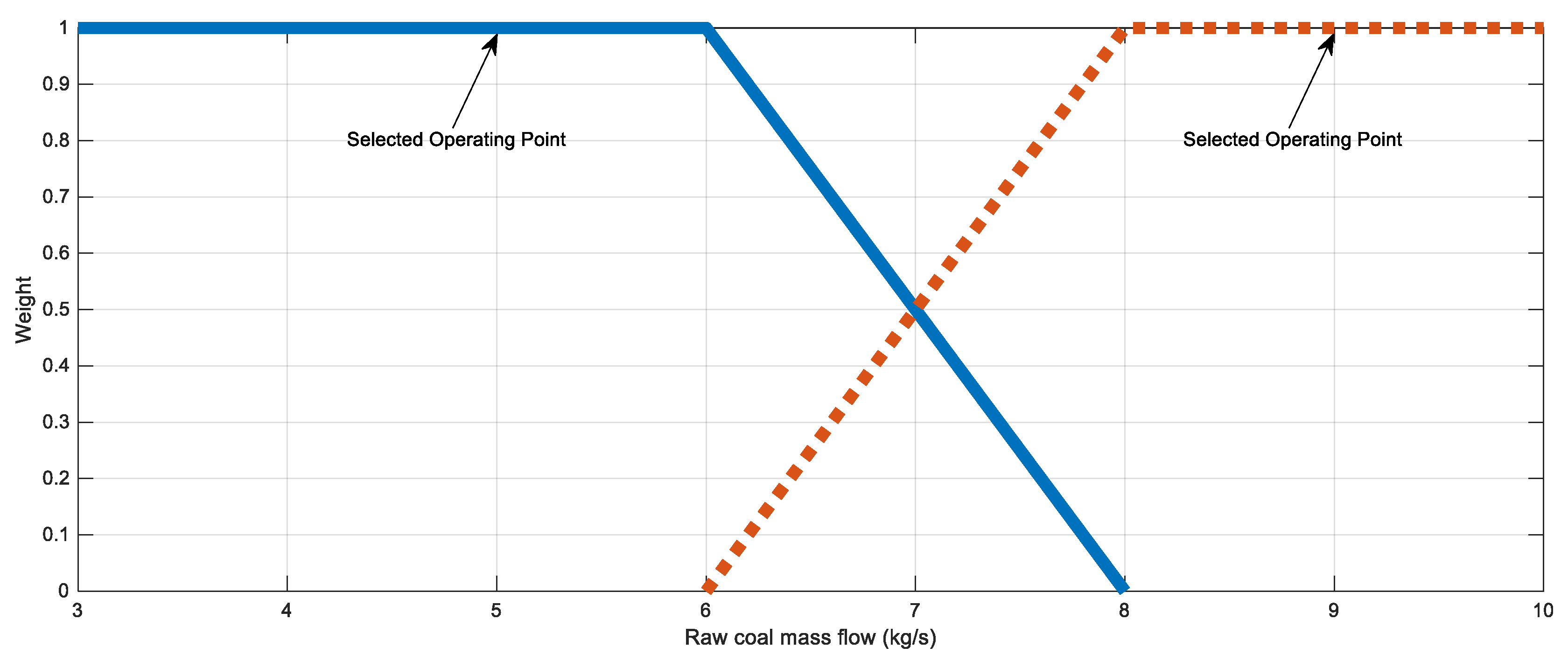
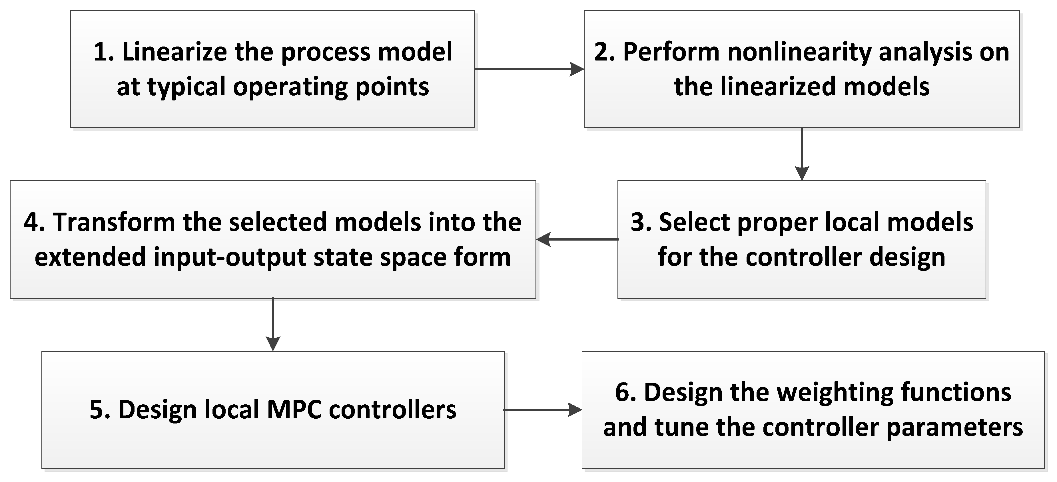
4.2. Multi-Model Predictive Controller Based on Extended Input-Output State Space Model

Modeling error and unknown disturbances always exist in practice. Therefore, integration must be included in the control algorithm. To achieve this, we can transform the original local linear models into the equivalent extended input-output state space for offset-free tracking performance [32,33]. In this control scheme, past values of the manipulated and controlled variables together with the tracking error form the new state variables. Therefore the method is free from the difficulties of observer based control techniques, such as convergence rate and observer robustness [32]. When the pulverizing system operates over a wide range, a single linear model for the MPC design will cause model discrepancies due to nonlinearities, with consequential control performance degradation. Therefore, two local MPC controllers were assigned with different operating ranges according the nonlinearity analysis. The proposed controller algorithm for the pulverizing system is as follows:

The selected local linear models can be described using the input-output linear difference model:

$$\begin{array}{l}y(k+1)+F_{1}y(k)+F_{2}y(k-1)+\dots +F_{n}y(k-n+1)\\ =H_{1}u(k)+H_{2}u(k-1)+\dots +H_{n}u(k-n+1)\end{array},$$

(57)

where $F_i\in R^{3\times 3}$, $H_i\in R^{3\times 6}$ (i = 1, 2, …, n), $y={\left[\begin{array}{ccc}{q}_{pul}& q_{air}& t_m\end{array}\right]}^T$ is the controlled variables, $u={\left[\begin{array}{cc}{u}_{mpc}^T& u_d^T\end{array}\right]}^T$ is the input variables, $u_{mpc}={\left[\begin{array}{ccc}{q}_{raw}& {\mu }_{cold}& {\mu }_{hot}\end{array}\right]}^T$ is the manipulated variables, and $u_d={\left[\begin{array}{ccc}{t}_{envi}& t_{cold}& t_{hot}\end{array}\right]}^T$ is the feed forward signal of measured disturbances. The local linear models are continuous and can be obtained by linearizing the model differential equations using first-order Taylor expansion.

Equation (57) can be transformed into the differenced form using the backshift operator, ∆:

$$\begin{array}{l}\Delta y(k+1)+F_1\Delta y(k)+F_2\Delta y(k-1)+\dots +F_n\Delta y(k-n+1)\\ =H_1\Delta u(k)+H_2\Delta u(k-1)+\dots +H_n\Delta u(k-n+1)\end{array},$$

(58)

where $\Delta y(i)=y(i)-y(i-1)$, $\Delta u(i)=u(i)-u(i-1)$.

We define the input–output states as:

$$\Delta x_m={\left[\begin{array}{cccccccc}\Delta y{(k)}^T& \Delta y{(k-1)}^T& \cdots & \Delta y{(k-n+1)}^T& \Delta u{(k-1)}^T& \Delta u{(k-2)}^T& \cdots & \Delta u{(k-n+1)}^T\end{array}\right]}^T$$

(59)

Thus, the corresponding state space model can be expressed as:

$$\{\begin{array}{l}\Delta x_m(k+1)=A_m\Delta x_m(k)+B_m\Delta u(k)\\ \Delta y(k)=C_m\Delta x_m(k)\end{array},$$

(60)

where:

$$A_m=\left[\begin{array}{ccccccccc}-F_1& -F_2& \cdots & -F_{n-1}& -F_n& H_2& \cdots & H_{n-1}& H_n\\ I& O& \cdots & O& O& O& \cdots & O& O\\ O& I& \cdots & O& O& O& \cdots & O& O\\ ⋮& ⋮& \cdots & ⋮& ⋮& ⋮& \cdots & ⋮& ⋮\\ O& O& \cdots & I& O& O& \cdots & O& O\\ O& O& \cdots & O& O& O& \cdots & O& O\\ O& O& \cdots & O& O& I& \cdots & O& O\\ ⋮& ⋮& \cdots & ⋮& ⋮& \cdots & ⋮& ⋮& ⋮\\ O& O& \cdots & O& O& O& \cdots & I& O\end{array}\right],$$

(61)

$$B_m=\left[\begin{array}{cccccccc}{H}_1^T& O& O& \cdots & O& I& O& O\end{array}\right]$$

(62)

and:

$$C_m=\left[\begin{array}{cccccccc}I& O& O& \cdots & O& O& O& O\end{array}\right]$$

(63)

Since the states are formed using input and output variables, the MPC controller does not require the design of state observers.

The output tracking error is defined as:

$$e(k)=y(k)-r(k),$$

(64)

where r(k) is the reference signal. Combining (60) and (64):

$$e(k+1)=e(k)+C_m{A}_m\Delta x_m(k)+C_m{B}_m\Delta u(k)-\Delta r(k+1),$$

(65)

by augmenting e(k) into the state variables and:

$$z(k)=\left[\begin{array}{c}\Delta x_m(k)\\ e(k)\end{array}\right].$$

(66)

The extended input–output state space model can be expressed as:

$$z(k+1)=Az(k)+B\Delta u(k)+C\Delta r(k+1),$$

(67)

where:

$$A=\left[\begin{array}{cc}{A}_m& 0\\ C_m{A}_m& I\end{array}\right],$$

(68)

$$B=\left[\begin{array}{c}{B}_m\\ C_m{B}_m\end{array}\right]$$

(69)

and:

$$C=\left[\begin{array}{c}0\\ -I\end{array}\right].$$

(70)

Note that when the system is in steady-state, the elements in z(k) must be zero and hence can guarantee y(k) = r(k), which indicates, using the extended input–output state space model as the prediction model in MPC, the desired controlled variables can track the reference signal with no offset.

The optimal control moves can be calculated by minimizing the objective function:

$$\begin{array}{c}\underset{\left\{\Delta u_{mpc}(k+i)i=1,2\dots ,M\right\}}{\arg \min }J={\displaystyle \sum _{j=1}^P{z}^T(k+j)Q_{j}z(k+j)+{\displaystyle \sum _{j=1}^M\Delta u^T(k+j)R_j\Delta u(k+j)}}\\ s.t.\{\begin{array}{l}\Delta u_{mpc}^{\max }\le \Delta u_{mpc}(k+i)\le \Delta u_{mpc}^{\min }\hspace{1em}\hspace{1em}0\le j<M\\ u_{mpc}^{\max }\le u_{mpc}(k+i)\le u_{mpc}^{\min }\hspace{1em}\hspace{1em}\hspace{1em}\hspace{1em}0\le j<M\\ \Delta u_{mpc}(k+i)=0\hspace{1em}\hspace{1em}\hspace{1em}\hspace{1em}\hspace{1em}\hspace{1em}\hspace{1em}\hspace{1em}j\ge M\end{array}\end{array},$$

(71)

where:

$$Q_j=diag\left\{q_{j,y1},q_{j,y2},q_{j,y3},q_{j,u1},q_{j,u2},\dots ,q_{j,u6},q_{j,e1},q_{j,e2},q_{j,e3}\right\};$$

(72)

$$R_j=diag\left\{\begin{array}{ccc}{r}_{j,u1}& r_{j,u2}& r_{j,u3}\end{array}\right\};$$

(73)

P and M are the prediction and control horizons, respectively; and $Q_j$ and $R_j$ are the weighting matrices. Generally, $q_{j,ei}$ (i = 1, 2, 3) and $r_{j,ui}$ (i = 1, 2, 3) cannot be set to zero, because the tracking error and control effort must be considered in the cost function.

Tuning of the MPC parameters is actually a compound problem owing to the lack of agreement on what satisfactory controller performance is [34]. Generally the weighting matrixes should be tuned based on practical needs. In the pulverizing system, since safe operation is the primary concern, the controller cannot take aggressive moves and hence $r_{j,ui}$ should be large enough to avoid overshot or oscillation of the controlled variables. To achieve this, we first fix $q_{j,ei}$ and then gradually increase $r_{j,ui}$ until overshot or oscillation disappears. In practice, the error weights $q_{j,ei}$ can be tuned empirically: if one or more process variables are more important than others, larger weights should be set on them to ensure the tracking performance [35]. We put more weights on the tracking error of primary air mass flow to maintain the economic air to coal ratio. The prediction and control horizons can be determined using empirical formulas proposed in [35].

Solving the optimization problem (71) for the two local controllers provides their control inputs, $U_1$ and $U_2$. Then the control move of the multi-model predictive controller can be expressed as:

$$u={\phi }_1{U}_1+{\phi }_2{U}_2,$$

(74)

where ${\phi }_1$ and ${\phi }_2$ are the weighting functions, and Figure 7 shows their relationship with the scheduling variable (raw coal mass flow). Trapezoidal relationship is employed owing to its simplicity in design. The switching points are placed at the 1/4 points on the line segment between the adjacent selected operating points, i.e., the 6 kg/s and 8 kg/s raw coal mass flowrate, so that the local controllers can switch smoothly.

The design procedures of the proposed MMPC are summarized in Figure 8.

5. Simulation Results

We tested the proposed inferential multi-model predictive control performance. The soft sensor effectiveness is presented first, and then the inferential multi-model control system is compared with proportional-integral (PI) control strategy for a real power plant.

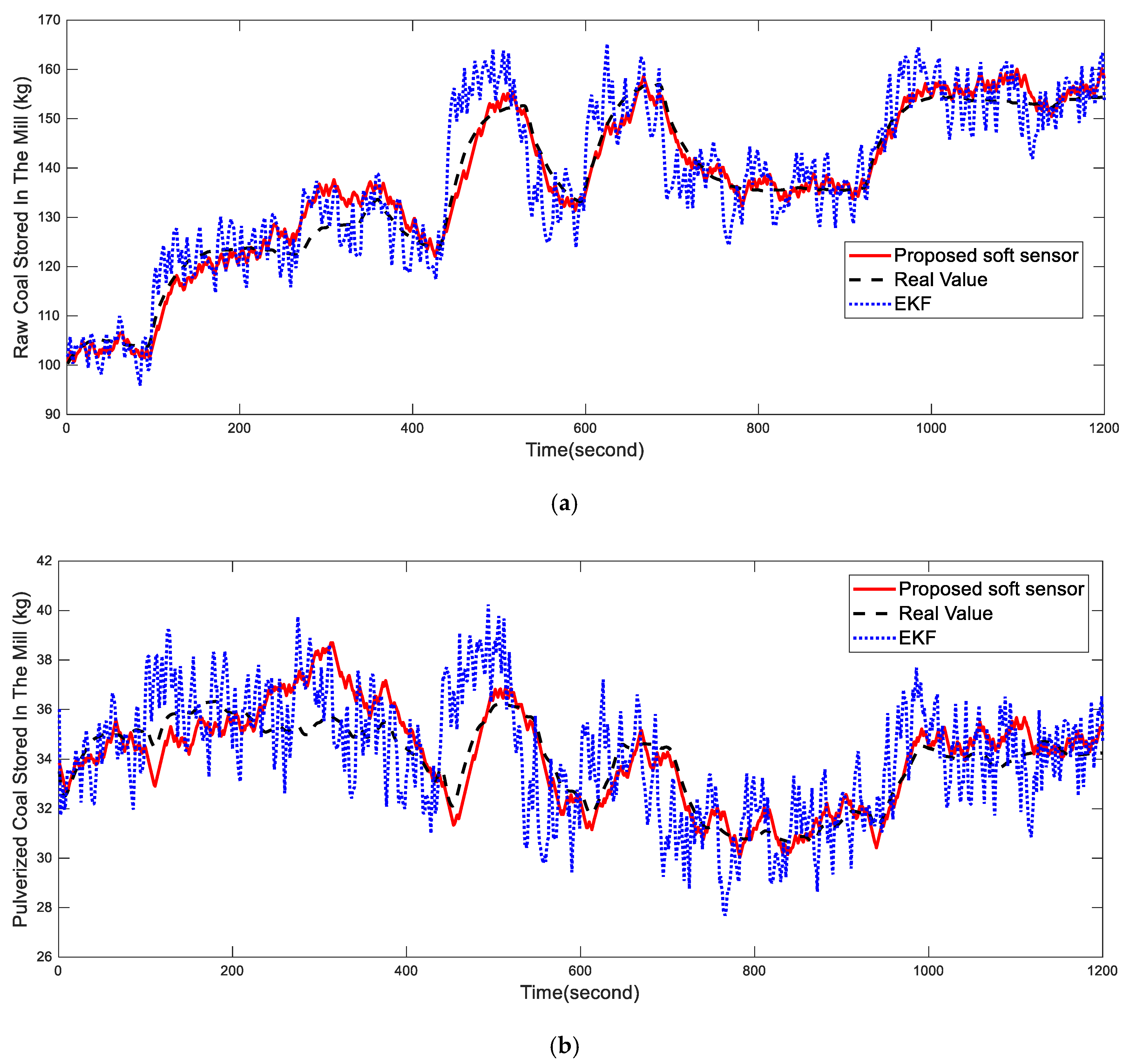
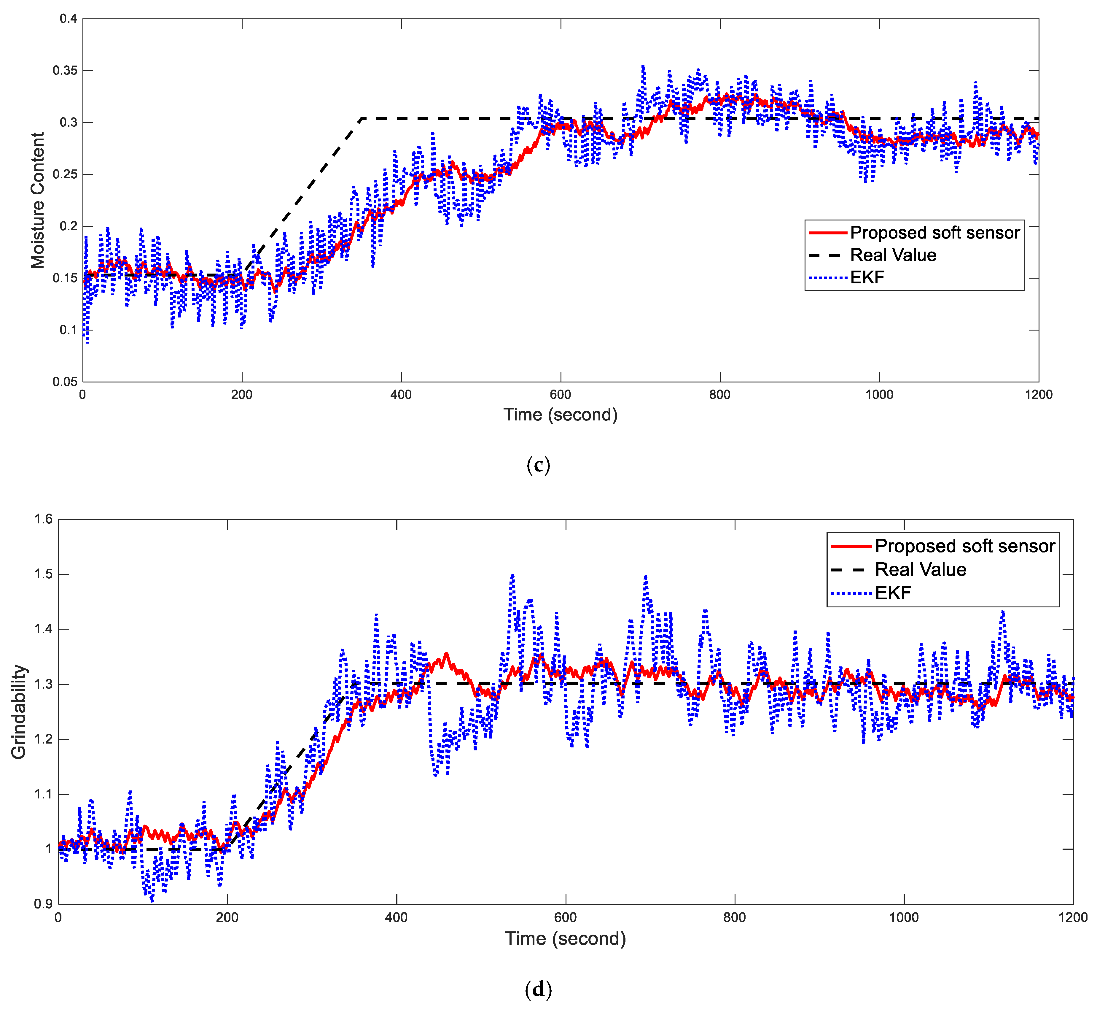
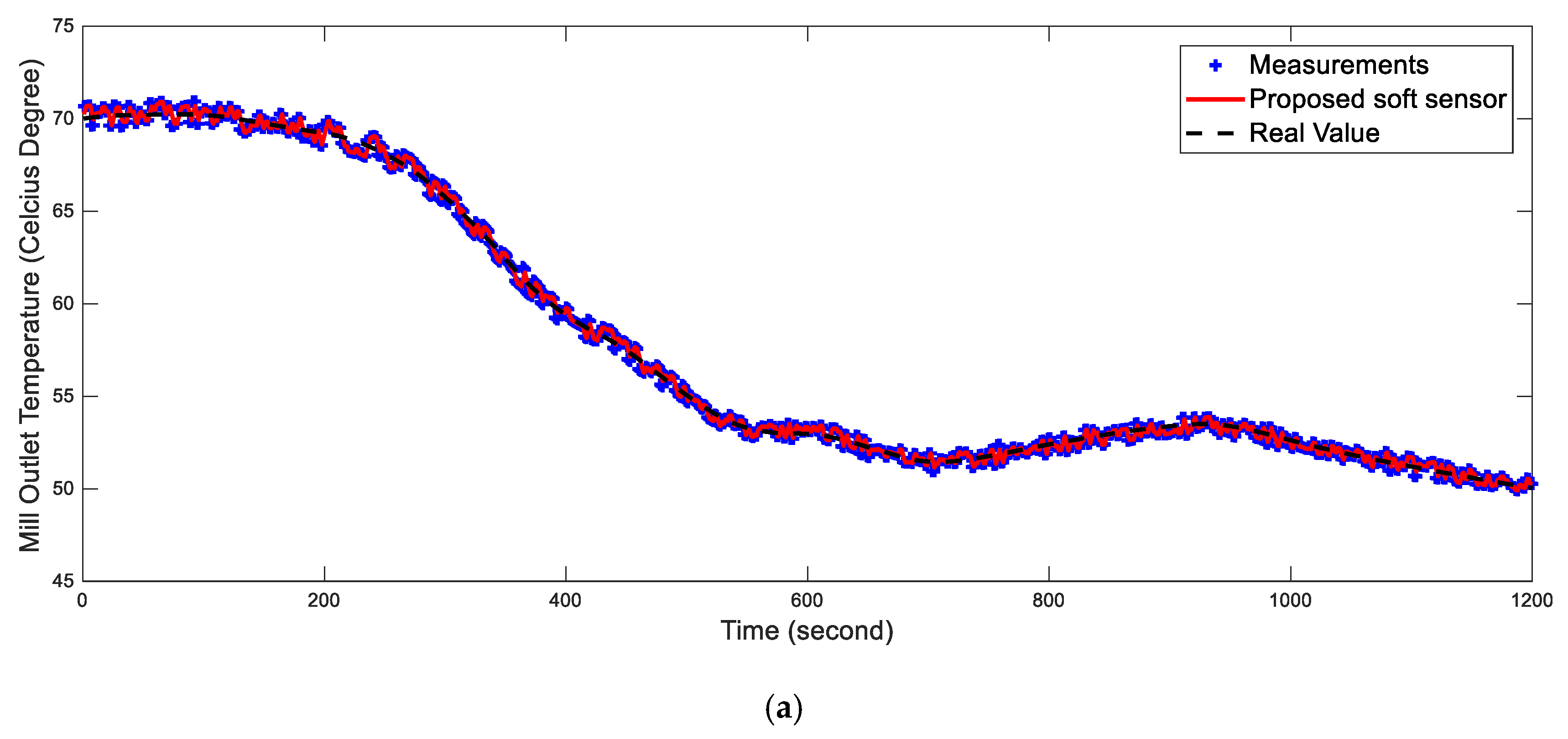
5.1. Soft Sensor Test

The proposed soft sensor was compared with a conventional extended Kalman filter (EKF), with the same weighting matrixes for states and outputs both cases. Sampling time for the soft sensor = 1 s, the same as the power plant DCS sampling time. Weighting matrixes in (27) were W = diag(0.5, 0.3, 0.1, 0.5, 0.5, 1), V = diag(1, 1, 10, 0.1, 5), which was a trade-off between model prediction and measurement data. Estimation horizon N = 10.

Table 5. State estimate constraints.

State Constraints	$\left|\Delta t_{air}(k,i)\right|$	$\left|\Delta q_{air}(k,i)\right|$	$\left|\Delta m_{raw}(k,i)\right|$	$\left|\Delta m_{pul}(k,i)\right|$	$\left|\Delta t_m(k,i)\right|$	$\left|\Delta \theta (k,i)\right|$	$\left|\Delta \eta (k,i)\right|$
Value	0.9 K/s	0.3 kg/s	0.5 kg/s	0.3 kg/s	0.2 K/s	0.01	0.01
Input Constraints	$\left|\Delta q_{raw}\right|$	$\left|\Delta {\mu }_{cold}\right|$	$\left|\Delta {\mu }_{hot}\right|$	$\left|\Delta t_{envi}\right|$	$\left|\Delta t_{cold}\right|$	$\left|\Delta t_{hot}\right|$
Value	0.05 kg/s	2%/s	2%/s	0.1 °C/s	0.1 °C/s	1.5 °C/s

shows the input and state estimate constraints, where k represents the present sample time, i represents the ith estimate in (27) (i = k − N+1, …, k), and ∆ means the difference between estimates at time k and k − 1. State constraints can be determined from the input constraints by simulating the first principle model.

As discussed earlier, raw coal and primary air mass flow cannot be accurately measured. Therefore, we set ±5% measurement uncertainty in the simulation, and ±1% measurement uncertainty for other input and output signals. Additionally, at 200 s we increased the raw coal moisture content and grindability to simulate the power plant changing raw coal type. Figure 9 shows unmeasurable states and parameters estimates, and Figure 10 shows controlled variables estimates. Since pulverized coal flow into the furnace is unmeasurable, the measured raw coal feed rate was also regarded as the pulverized coal flow for the simulation.

Table 6. RMS errors and 3-sigma error bounds of the estimates.

	Raw Coal Stored in the Mill	Pulverized Coal Stored in the Mill	Moisture Content	Grindability
RMS of MHE	2.8493	0.9084	0.0391	0.028
RMS of EKF	6.0084	1.8175	0.0417	0.0585
Error bound of EKF	±18.0326	±5.4549	±0.1253	±0.1757
Error bound of MHE	±8.5516	±2.7263	±0.1172	±0.0839

shows the root-mean-square (RMS) errors and 3-sigma error bounds of the estimates for MHE and EKF.

Figure 9 and Table 6 show that the proposed soft sensor provides satisfactory unmeasurable states and parameter estimates in the presence of measurement uncertainty. Since the state constraint is considered, which represents prior knowledge of the process, the proposed soft sensor is less affected by measurement uncertainty than EKF. Previous studies have shown that, given the same tuning parameters, MHE can provide improved estimates and greater robustness than EKF [36], which is verified by the current simulation.

Raw coal property changes were successfully detected by the soft sensor. Therefore, when the power plant changes raw coal type, we can slowly update the model parameters online rather then re-identifying the model parameters. There was a large delay between real and estimated moisture content, since the changed moisture content only influences outlet temperature slowly due to the large energy balance inertia, hence the true value cannot be immediately estimated.

Figure 10 shows that pulverized coal flow into the furnace and primary air flow estimates are significantly closer to the real values than were the measurements, and outlet temperature estimates had similar precision to the measurements. Since the outlet temperature is already measured accurately, the soft sensor cannot significantly improve its measurement accuracy. However, the other two controlled variables are only approximately measured, and the soft sensor can significantly improve their measurement quality because it employs accurately measured signals to reconstruct measurement signals based on the first principle model. Therefore, using estimates rather than measurements as the control system feedback signal can significantly enhance control precision of the desired controlled variables.

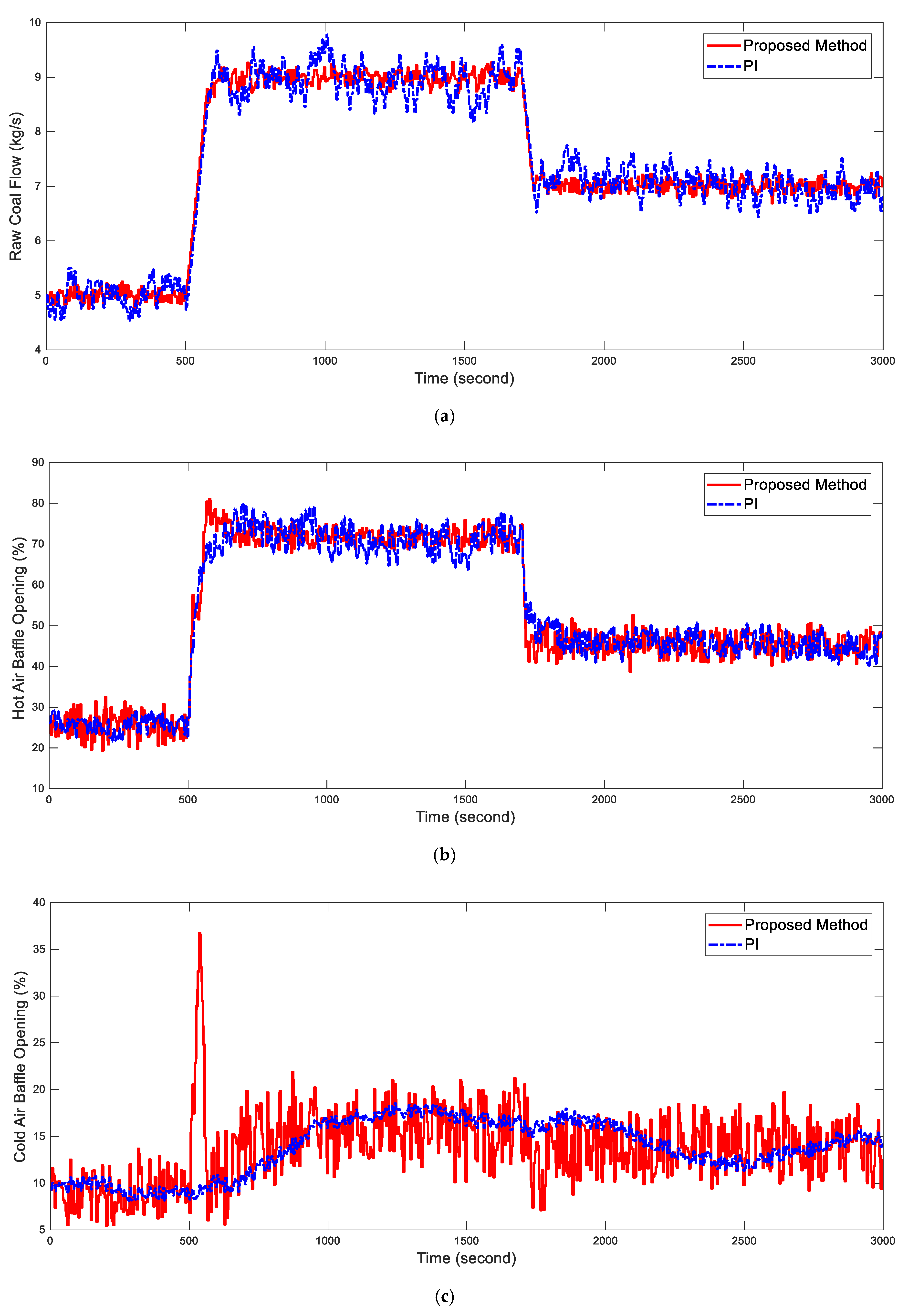
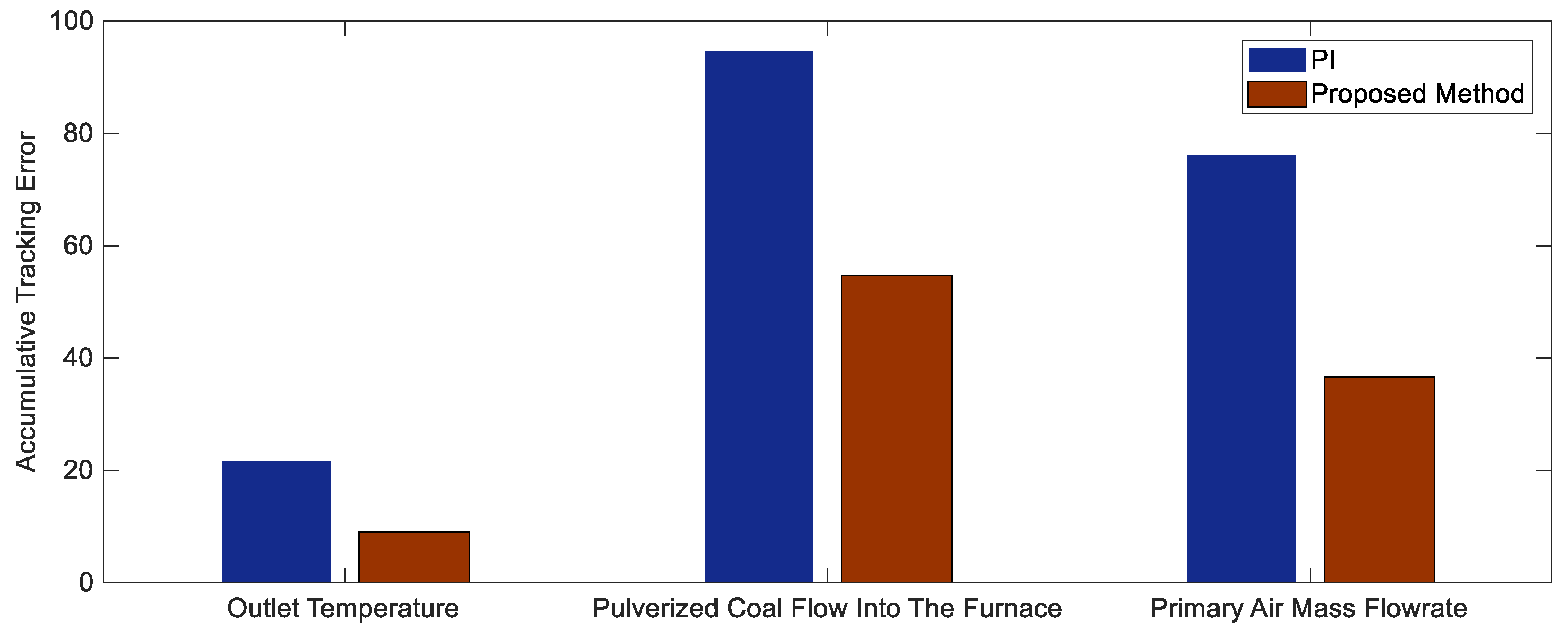
5.2. Inferential Control Strategy Test

We tested tracking performance of the proposed inferential multi-model predictive controller. Measurement uncertainty was set the same as the previous simulation, and sample time for the controller = 5 s due to the large process inertia. We set $q_{j,yi}=0$ (i = 1, 2, 3) and $q_{j,ui}=0$ (i = 1, 2, …, 8) to simplify (71), which also means that only tracking error and control effort were considered. The weights for tracking error and control effort were $q_{j,y1}$ = 4, $q_{j,y2}$ = 8, $q_{j,y3}$ = 1, $q_{j,u1}$= 60, $q_{j,u2}$ = 10, and $q_{j,u3}$ = 10. Prediction horizon = 100, long enough to cover key pulverizing system dynamics. Tuning the control horizon was a trade-off between computation cost and control performance [37], and was set = 5.

In real power plants, the pulverizing system is controlled via three independent single PI control loops, which are tuned conservatively to ensure safe and reliable operation [6]. Hence the PI controllers were employed to compare with proposed control system. Figure 11 shows the PI control structure used for comparison, and Figure 12 shows the simulation results. Note that, in the PI control scheme, the pulverized coal flow into the furnace is estimated by solving the model differential equations given the input signals.

To investigate control performance quantitatively, we introduce the cumulative tracking error:

$${\displaystyle \sum _{i=1}^T\left|\frac{y_{real}^i-y_{ref}^i}{y_{ref}^i}\right|},$$

(75)

where T is the total simulation time, and subscripts ref denotes the reference signal and real denotes the real controlled variable value. Figure 12 shows the cumulative tracking error for the proposed and PI controllers.

Figure 12 and Figure 13 show that the proposed multi-model inferential controller can significantly improve pulverizing system control precision and tracking performance over a wide operating range. The reasons for this good performance are summarized as follows.

(1)

The desired controlled variables are more accurately “measured” by the soft sensor, hence their control precision is significantly improved. The proposed control scheme produces fewer fluctuations around its set point for mass flowrate of primary air and pulverized coal into the furnace, which indicates that the inferential controller is less sensitive to measurement uncertainty.

(2)

The multi-model MPC controller can automatically handle nonlinearity, large inertia, and coupling effects of the pulverizing system. At 500 s, the power plant coal demand increased to 9 kg/s. Since the predictive controller can foresee the future outlet temperature increment, it opens the cold air baffle in advance to compensate for the excess energy input by the hot air. Hence temperature is successfully maintained around 70 °C. A similar result is observed at 1700 s, where coal demand falls to 7 kg/s. The PI controller cannot predict the influence from other control loops and handle it timely, resulting in poorly controlled outlet temperature. The PI controller can also easily result in oscillatory performance, due to the large energy balance inertia.

Since the pulverized coal flow into the furnace is more accurately controlled within the proposed control scheme, the power plant load will have fewer fluctuations caused by measurement uncertainty. Primary air also tracks the set point faster than the PI controller, which indicates that the air to coal ratio is better controlled. The outlet temperature exhibits almost no oscillations, showing that safe operation of the system has been improved.

6. Conclusions

This paper proposed an inferential multi-model predictive control method to improve pulverizing system control precision and tracking performance. A first principle model of the pulverizing system was developed considering primary air nonlinear dynamics. The proposed model also considered the grindability and moisture content of raw coal to adapt to the change of raw coal type. The unknown parameters in the pulverizing system model were identified using a genetic algorithm. Model validation showed that the proposed model agreed well with measurement data from a real plant, and hence it was employed as the simulation platform for the design of soft sensor and inferential controller.

A soft sensor was developed based on the established model using an MHE approach to estimate desired controlled variables that are unmeasurable or inaccurately measured. The proposed soft sensor can reconstruct signals of the desired controlled variables from more accurately measured variables and thus can improve their “measurement” accuracy. Moreover constraints in the estimates were explicitly considered in the MHE, such that the influence of measurement uncertainty can be significantly reduced. To improve accuracy and computation speed of the MHE, we derived an efficient arrival cost update based on the pulverizing system model. Simulation results showed that the proposed soft sensor can give improved estimates compared with conventional EKF.

Estimated outputs of the soft sensor were employed as feedback signals for an inferential multi-model predictive controller, because, as shown in simulation results, the estimates were much closer to the real value than measurements. We analyzed nonlinearity of the pulverizing system using gap metric and then selected two linear models to construct the local MPC controller based on the analysis. To achieve offset free performance in the presence of unknown disturbances and modeling error, the local linear models were transformed into the extended input-output state space model for controller design. The proposed controller was compared with conventional PI controllers applied in real power plants. Simulation results showed that the proposed inferential method could significantly improve control precision and tracking performance of pulverized coal flow into the furnace, primary air mass flow and outlet temperature.

References

1. Flynn, D. Thermal Power Plant Simulation and Control; IET: London, UK, 2003. [Google Scholar]
2. Bhatt, M.S. Effect of air ingress on the energy performance of coal fired thermal power plants. Energy Convers. Manag. 2007, 48, 2150–2160. [Google Scholar] [CrossRef]
3. Agrawal, V.; Panigrahi, B.K.; Subbarao, P.M.V. Review of control and fault diagnosis methods applied to coal mills. J. Process Control 2015, 32, 138–153. [Google Scholar] [CrossRef]
4. Agrawal, V.; Panigrahi, B.K.; Subbarao, P.M.V. A unified thermo-mechanical model for coal mill operation. Control Eng. Pract. 2015, 44, 157–171. [Google Scholar] [CrossRef]
5. Wu, Y.; Wu, X.; Wang, Z.; Chen, L.; Cen, K. Coal powder measurement by digital holography with expanded measurement area. Appl. Opt. 2011, 50, 22–29. [Google Scholar] [CrossRef] [PubMed]
6. Gao, Y.; Zeng, D.; Liu, J.; Jian, Y. Optimization control of a pulverizing system on the basis of the estimation of the outlet coal powder flow of a coal mill. Control Eng. Pract. 2017, 63, 69–80. [Google Scholar] [CrossRef]
7. Iii, F.J.D. Nonlinear inferential control for process applications. J. Process Control 1998, 8, 339–353. [Google Scholar]
8. Niemczyk, P.; Bendtsen, J.D.; Ravn, A.P.; Andersen, P.; Pedersen, T.S. Derivation and validation of a coal mill model for control. Control Eng. Pract. 2012, 20, 519–530. [Google Scholar] [CrossRef]
9. Jin, A.; Hitotumatu, S.; Sato, I. Modeling and Parameter Identification of Coal Mill. J. Power Electron. 2009, 9, 700–707. [Google Scholar]
10. Zeng, D.L.; Hu, Y.; Gao, S.; Liu, J.Z. Modelling and control of pulverizing system considering coal moisture. Energy 2015, 80, 55–63. [Google Scholar] [CrossRef]
11. Wei, J.L.; Wang, J.; Wu, Q.H. Development of a Multisegment Coal Mill Model Using an Evolutionary Computation Technique. IEEE Trans. Energy Convers. 2007, 22, 718–727. [Google Scholar] [CrossRef]
12. Lu, J.; Chen, L.; Shen, J.; Wu, Y.; Lu, F. A study of control strategy for the bin system with tube mill in the coal fired power station. ISA Trans. 2002, 41, 215–224. [Google Scholar] [CrossRef]
13. Fei, M.; Zhang, J. Robust Fuzzy Tracking Control Simulation of Medium-speed Pulverizer. In Systems Modeling and Simulation; Springer: Heidelberg, Germany, 2007. [Google Scholar]
14. Cortinovis, A.; Mercangöz, M.; Mathur, T.; Poland, J.; Blaumann, M. Nonlinear coal mill modeling and its application to model predictive control. Control Eng. Pract. 2013, 21, 308–320. [Google Scholar] [CrossRef]
15. Song, G.L.; Zhou, J.H.; Weng, W.G. Experimental Research on Cold Aerodynamic Field of 75t/h Boiler with Tangential Firing. Power Syst. Eng. 2005, 21, 14–16. [Google Scholar]
16. The Engineering ToolBox. Available online: https://www.engineeringtoolbox.com/control-valves-flow-characteristics-d_485.html (accessed on 23 January 2018).
17. Kachitvichyanukul, V. Comparison of three evolutionary algorithms: GA, PSO, and DE. Ind. Eng. Manag. Syst. 2012, 11, 215–223. [Google Scholar] [CrossRef]
18. Rashtchi, V.; Rahimpour, E.; Rezapour, E.M. Using a genetic algorithm for parameter identification of transformer RLCM model. Electr. Eng. 2006, 88, 417–422. [Google Scholar] [CrossRef]
19. Wang, J.; Wang, J.; Daw, N.; Wu, Q. Identification of pneumatic cylinder friction parameters using genetic algorithms. IEEE/ASME Trans. Mechatron. 2004, 9, 100–107. [Google Scholar] [CrossRef]
20. Zhang, Y.G.; Wu, Q.H.; Wang, J.; Oluwande, G. Coal Mill Modeling by Machine Learning Based on on-Site Measurements. IEEE Trans. Energy Convers. 2002, 17, 549–555. [Google Scholar] [CrossRef]
21. Ghosh, A. Evolutionary Computation in Data Mining; Springer: Heidelburg, Germany, 2004. [Google Scholar]
22. Pachauri, N.; Singh, V.; Rani, A. Two degree of freedom PID based inferential control of continuous bioreactor for ethanol production. ISA Trans. 2017, 68, 235–250. [Google Scholar] [CrossRef] [PubMed]
23. Darko, S.I.; Nikola, J.; Nikola, P.; Velimir, O. Soft sensor for real-time cement fineness estimation. ISA Trans. 2015, 55, 250–259. [Google Scholar]
24. Rani, A.; Singh, V.; Gupta, J.R. Development of soft sensor for neural network based control of distillation column. ISA Trans. 2013, 52, 438–449. [Google Scholar] [CrossRef] [PubMed]
25. Zhai, Y.J.; Yu, D.L.; Qian, K.J.; Lee, S.; Theera-Umpon, N. A Soft Sensor-Based Fault-Tolerant Control on the Air Fuel Ratio of Spark-Ignition Engines. Energies 2017, 10, 131. [Google Scholar] [CrossRef]
26. Zhang, D.; Liu, G.; Zhao, W.; Miao, P.; Jiang, Y.; Zhou, H. A Neural Network Combined Inverse Controller for a Two-Rear-Wheel Independently Driven Electric Vehicle. Energies 2014, 7, 4614–4628. [Google Scholar] [CrossRef]
27. Rao, C.V.; Rawlings, J.B.; Lee, J.H. Constrained linear state estimation—A moving horizon approach. Automatica 2001, 37, 1619–1628. [Google Scholar] [CrossRef]
28. Rao, C.V.; Rawlings, J.B.; Mayne, D.Q. Constrained state estimation for nonlinear discrete-time systems: Stability and moving horizon approximations. IEEE Trans. Autom. Control 2003, 48, 246–258. [Google Scholar] [CrossRef]
29. Lopez-Negrete, R.; Patwardhan, S.C.; Biegler, L.T. Constrained particle filter approach to approximate the arrival cost in moving horizon estimation. J. Process Control 2011, 21, 909–919. [Google Scholar] [CrossRef]
30. Kühl, P.; Diehl, M.; Kraus, T.; Schlöder, J.P.; Bock, H.G. A real-time algorithm for moving horizon state and parameter estimation. Comput. Chem. Eng. 2011, 35, 71–83. [Google Scholar] [CrossRef]
31. Du, J.; Song, C.; Yao, Y.; Li, P. Multilinear model decomposition of MIMO nonlinear systems and its implication for multilinear model-based control. J. Process Control 2013, 23, 271–281. [Google Scholar] [CrossRef]
32. Zhang, R.; Xue, A.; Wang, S.; Ren, Z. An improved model predictive control approach based on extended non-minimal state space formulation. J. Process Control 2011, 21, 1183–1192. [Google Scholar] [CrossRef]
33. Wang, L.; Young, P.C. An improved structure for model predictive control using non-minimal state space realisation. J. Process Control 2006, 16, 355–371. [Google Scholar] [CrossRef]
34. Gous, G.Z.; De Vaal, P.L. Using MV overshoot as a tuning metric in choosing DMC move suppression values. ISA Trans. 2012, 51, 657–664. [Google Scholar] [CrossRef] [PubMed]
35. Garriga, J.L.; Soroush, M. Model predictive control tuning methods: A review. Ind. Eng. Chem. Res. 2010, 49, 3505–3515. [Google Scholar] [CrossRef]
36. And, E.L.H.; Rawlings, J.B. Critical Evaluation of Extended Kalman Filtering and Moving-Horizon Estimation. Ind. Eng. Chem. Res. 2005, 44, 2451–2460. [Google Scholar]
37. Wu, X.; Shen, J.; Li, Y.; Lee, K.Y. Fuzzy modeling and stable model predictive tracking control of large-scale power plants. J. Process Control 2014, 24, 1609–1626. [Google Scholar] [CrossRef]
Figure 1. Simplified diagram of a typical pulverizing system.
Energies 11 00589 g001
Figure 2. Typical inherent valve characteristics [16].
Energies 11 00589 g002
Figure 3. Identification process of GA.
Energies 11 00589 g003
Figure 4. Validation of the proposed pulverizing system model. (a) Primary air temperature; (b) Primary air mass flow; (c) Electric current; (d) Outlet temperature; (e) Differential pressure.
Energies 11 00589 g004aEnergies 11 00589 g004bEnergies 11 00589 g004c
Figure 5. Inferential control system structure.
Energies 11 00589 g005
Figure 6. Gap metric between local linear models.
Energies 11 00589 g006
Figure 7. Weighting functions and scheduling variable: φ 1 = solid line, φ 2 = dotted line.
Energies 11 00589 g007
Figure 8. Design procedures of proposed MMPC.
Energies 11 00589 g008
Figure 9. Estimates of (a,b) unmeasurable states and (c,d) raw coal parameters. (a) Raw coal stored in the mill; (b) Pulverized coal stored in the mill; (c) Moisture content; (d) Grindability.
Energies 11 00589 g009aEnergies 11 00589 g009b
Figure 10. Controlled variable estimates. (a) Mill outlet temperature; (b) Primary air mass flow; (c) Pulverized coal flow into the furnace.
Energies 11 00589 g010aEnergies 11 00589 g010b
Figure 11. Conventional PI control structure.
Energies 11 00589 g011
Figure 12. Proposed and PID control method performances for (ac) control inputs, and (df) controlled outputs. (a) Raw coal flow; (b) Hot air baffle opening; (c) Cold air baffle opening; (d) Pulverized coal into the furnace; (e) Primary air mass flow; (f) Outlet temperature.
Energies 11 00589 g012aEnergies 11 00589 g012b
Figure 13. Cumulative tracking error.
Energies 11 00589 g013