Impulsive Noise Characterization in Narrowband Power Line Communication

Abstract

Currently, narrowband Power line communication (PLC) is considered an attractive communication system in smart grid environments for applications such as advanced metering infrastructure (AMI). In this paper, we will present a comprehensive comparison and analysis in time and frequency domain of noise measured in China and Italy. In addition, impulsive noise in these two countries are mainly analyzed and modeled using two probability based models, Middleton Class A (MCA) model and $\alpha$ stable distribution model. The results prove that noise measured in China is rich in impulsive noise, and can be modeled well by $\alpha$ stable distribution model, while noise measured in Italy has less impulsive noise, and can be better modeled by the MCA model.

1. Introduction

Power Line Communications (PLC), is currently considered an attractive communication system in smart grid because of its ubiquitous infrastructure and low-cost operation maintenance. Advanced metering infrastructure (AMI), based on narrowband PLC, can be applied in automatic meter reading (AMR), demand side response, real-time monitoring and vehicle charging in the smart grid. It is well known that the PLC channel is a hostile medium for communication due to its multi-path effect, time varying properties and strong noise interference.

For widespread narrowband PLC, four unified international standards are developed including PRIME, G3, IEEE P1901.2 and G.HNEM. According to the CENELEC (European Committee for Electrotechnical Standardization) frequency bands, all these four standards are applied in CENELEC A band (35.9–90.6 kHz), while the utilization of the U.S. Federal Communication Commission (FCC) band is shown in

Table 1. Frequency bands applied in four Narrowband PLC standards in Europe and USA

Frequency Range	PRIME	G3	IEEE P1901.2	G.HNEM
CEN A	42–89 kHz	39.9–90.6 kHz	39.9–90.6 kHz	39.9–90.6 kHz
FCC	/	159.4–478.1 kHz	35.9–487.5 kHz	34.4–478.1 kH

.

An overview of the noise characteristics in narrowband PLC can be found in [1,2]. The available noise measurements have been carried out in distributed networks of different topologies in some countries, but they are conducted only in partial sub-bands of 3–500 kHz, instead of covering the whole frequency band. In addition, noise measurements of many in-home devices (dimmers, universal motors, PC, etc.) have also been conducted in order to model the noise characteristics. For instance, see data for China [3], Brazil [4], USA [5,6,7,8], Germany [9,10], France [5], Tunisia [11,12], Sweden [13], Japan [14] and Italy [15]. However, when collecting these available noise data, the measurement set-up is not always presented in a comprehensive manner.

Power line noise was firstly measured in frequency band of 0–100 kHz, and classified into different types based on its characteristics in time and frequency domain [5]. According to [5], power line noise in broadband PLC lower than 20 MHz was first categorized into five classes: colored background noise (CBG), narrowband interferences (NBI), periodic impulsive noise synchronous to mains frequency (PINS), periodic impulsive noise asynchronous to the mains frequency (PINAS) and asynchronous impulsive noise (AIN) in [16]. An empirical noise model was built based based on time and frequency domain observation, especially defining the basic characteristics of impulsive noise such as impulse width, impulsive amplitude, interarrival time, impulse rate and the disturbance ratio. This noise classification was comprehensively applied in subsequent power line noise modeling in both broadband and narrowband PLC [17]. Generally, the three types of impulsive noise (PIN, PINAS and AIN) are modeled as a single group (impulsive noise, IN) in broadband PLC, because of their fast time varying behaviour. This is due to the fact that, in broadband PLC, the time duration of one OFDM (Orthogonal Frequency Division Multiplexing) symbol or frame is far shorter than one mains period, thus the cyclostationary property is seldom considered. In [18], impulsive noise was modeled in frequency domain considering the channel transfer characteristics between noise source and receiver. In [19], based on physical and statistical properties of impulsive noise such as in [16], impulsive noise was modeled by starting with a specific noise measurement. Power line noise in narrowband PLC was also modeled considering the noise taxonomy proposed above [20]. However, in narrowband PLC the time duration of one OFDM frame lasts longer than one mains period. For example, in PRIME protocol the time duration of one OFDM frame is high up to 145.65 ms and 581.63 ms of two different frame types. In IEEE P1901.2 standard one typical data frame lasts 9.44 ms. Therefore, the cyclostationary behavior has been examined in more detail [21,22,23]. The modeling methods above are based on noise physical characteristics in specific scenarios.

On the other hand, another way to describe the power line noise characteristics is based on the use of probability distribution, in which MCA model and $\alpha$ stable distribution are applied. Among all five classes of noise, NBI in broadband PLC is generally caused by radio waves, and is not considered in these methods. Besides, the three kinds of impulsive noise are considered together, instead of being modeled separately. Therefore, power line noise modeling based on probability distribution mainly attempts to characterize impulsive noise. The MCA model was proposed to describe natural or man-made electromagnetic disturbance, in which noise is mainly spectrally narrower compared to the receiver bandwidth [24]. Its probability density function (PDF) can be determined by only three factors: impulse index, the variance of background Gaussian noise to that of the impulsive power ratio, and background Gaussian noise variance, which makes it widely used in power line impulsive noise modeling. However, it fails to characterize noise temporary property, Markov-Middleton Model (MM) was proposed to characterize impulsive noise bursts, but they still share the same PDF [25]. Furthermore, it is proved that power spectrum density (PSD) of MCA model and Markov Middleton Model are similar and close to PSD of white noise [26]. The $\alpha$-stable distribution model was commonly employed to model impulsive noise in various physical environments including underwater acoustic noise, man-made audio noise, as well as different types of electromagnetic phenomena [27]. It was used to characterize power line impulsive noise in industrial zone [28] and in other scenarios based on measurement in frequency band of 0–50 kHz in CEN A [29,30]. The $\alpha$-stable distribution has not yet been examined for the whole frequency band in narrowband PLC.

In this paper, power line noise indoors were measured both in China and Italy with different loads connected to the network, and the frequency range nearly embraces the whole frequency band of 30–500 kHz. We propose a statistical study of the main characteristics of the measured noise in both countries: we compare the basic noise characteristics both in time and frequency domain of two countries and apply two noise modeling techniques (MCA and $\alpha$-stable distribution) as well as inspecting their sustainability.

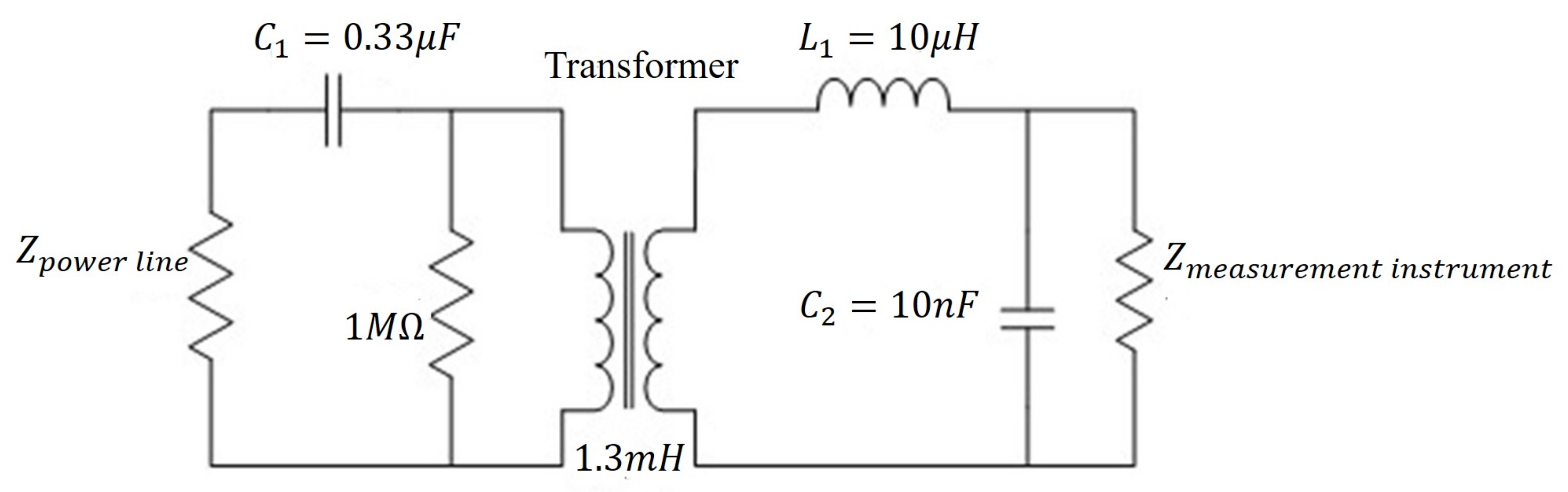
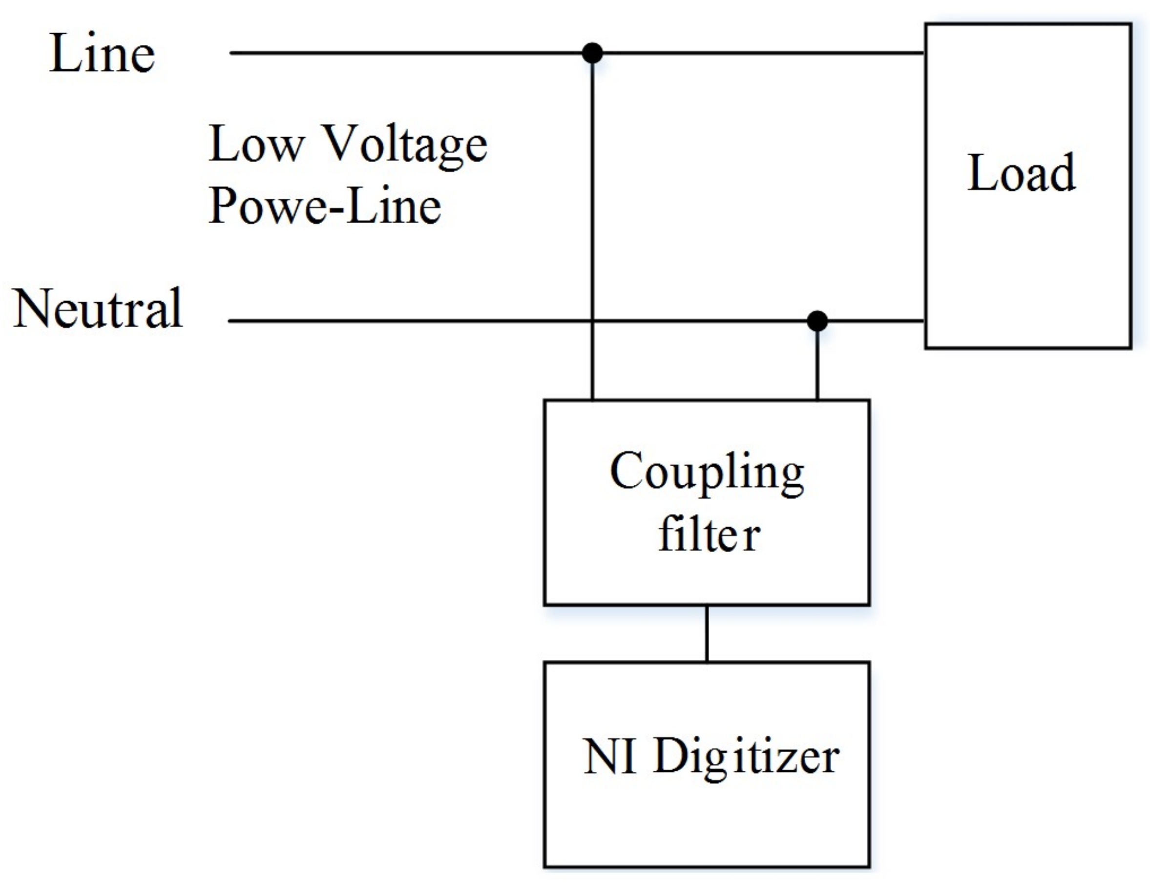
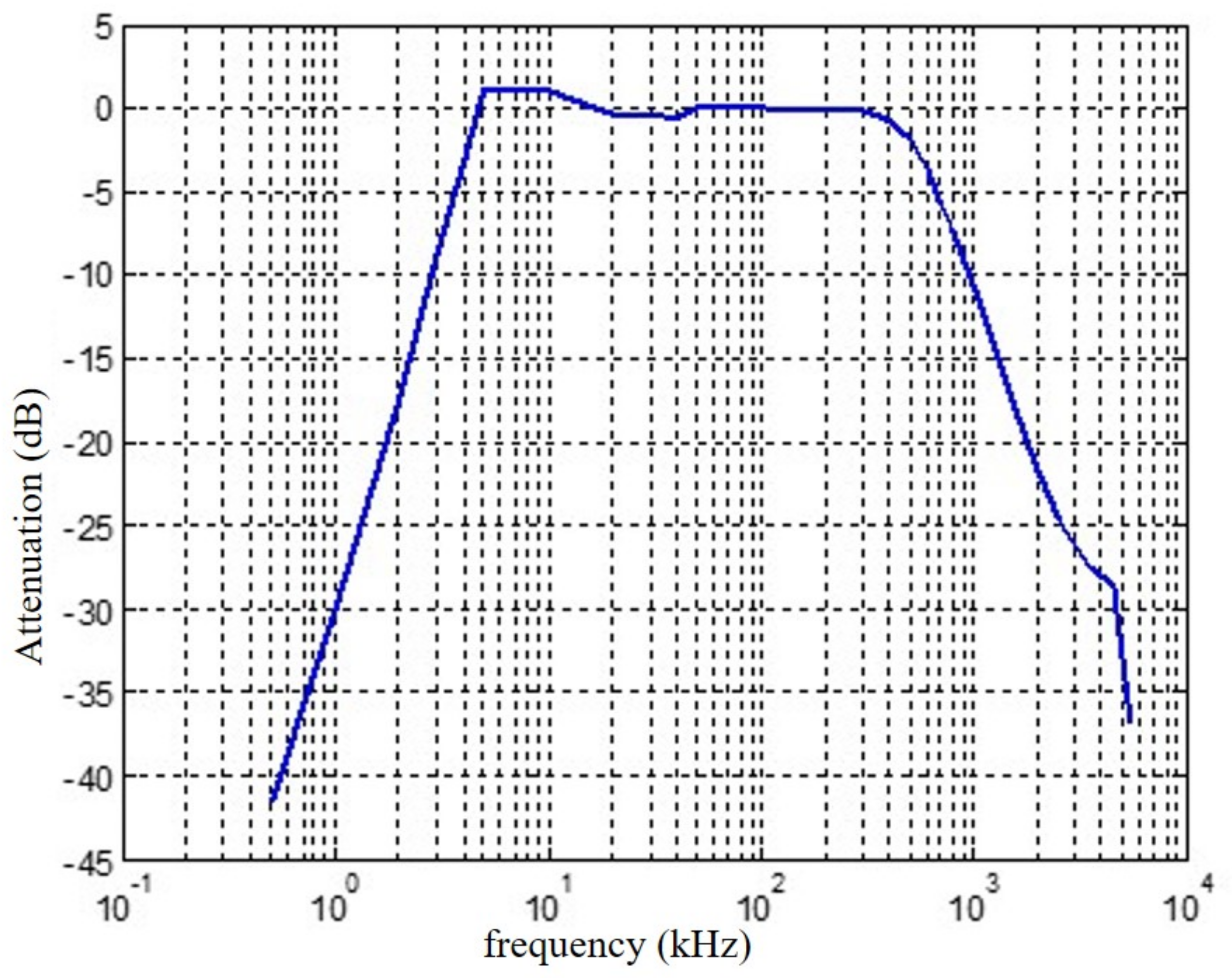
2. Measurement Setup in China and Itlay

The measurement setup is shown in Figure 1. The main measurement instrument is a PXI digitizer (National Instrument). A PXI 5105 was used in China, whereas a PXI 5124 was used in Italy. Both digitizers have 12-bit resolution, and the maximum sampling speed is above 50 MS/s. The digitizer was connected to the low voltage network of 220 V through a coupling filter and a digital signal processing software, LabVIEW, was used to record and process the collected data. The coupling filter circuit used in China is shown in Figure 2, and its measured transfer function is shown in Figure 3. The coupling filter used in Italy is similar, and it is described in [31]. In both cases the coupling filter acts as a band pass filter, with a 3 dB attenuation in the band between 4 kHz (7 kHz in Italy) and 600 kHz, resulting in a large attenuation of the 50 Hz mains frequency. As explained before we focused on narrowband PLC noise measurement in the frequency range from 10 kHz to 600 kHz, a sampling frequency of 2 MS/s is adopted in the measurement in both countries.

In order to evaluate power line noise injected in the low voltage network by commonly used devices, a great number of measurements have been done with different loads connected to different locations in each environment such as home and lab. Different loads are connected to the same multi-socket where the measurement setup is connected. The scope of this arrangement is to measure the noise that a narrowband PLC device would receive from the network when it is connected near to a commonly used device, in home or office environments.

In China, measurements were carried out in both lab and home environments with different loads and locations. In the lab environment, power line noises of cellphone charger, hairdryer, screen and PC were collected with two locations respectively, while in the home environment, fridge, TV and washing machine were used for noise collection in three locations. In Italy, measurements were carried out with four locations in home environment, and the measured devices were vacuum cleaner, 1A cellphone charger, washing machine, hairdryer, microwave oven, 19A laptop charger, 32 inch led TV, fridge, coffee machine and a charger for electric tooth cleaner that both use wireless power transfer (WPT) technology. In detail, cellphone charger, screen, TV and PC are rectifier loads, WPT is inductive load, fridge, washing machine and coffee machine are motor loads and hairdryer is resistive load. Moreover, microwave oven contains rectifier and inductive loads. With a great number of measurements on different occasions, the noise comparison will be conducted comprehensively and generally.

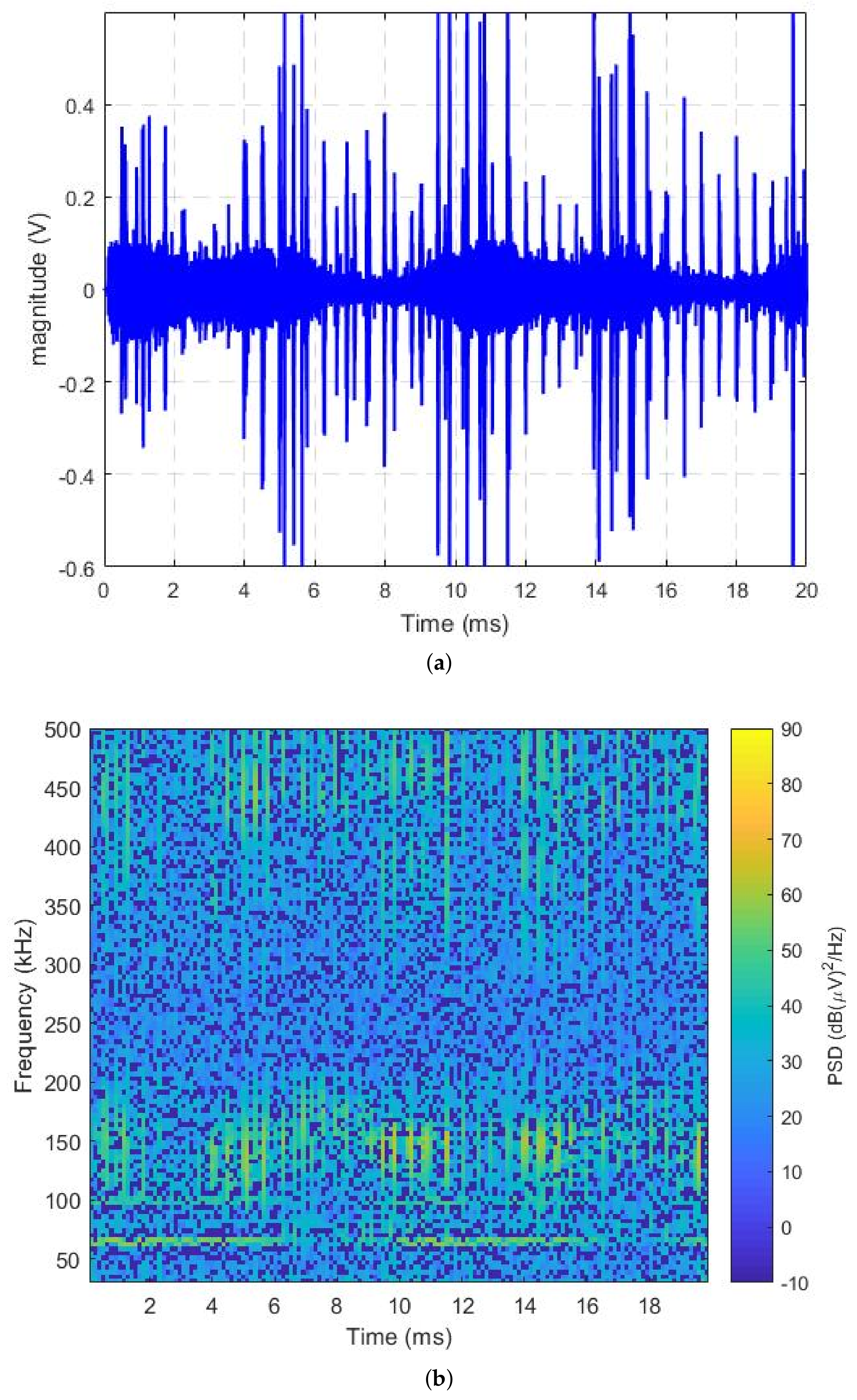
3. Basic Time and Frequency Domain Analysis of Noise

The noise data are collected in both countries in the frequency range of 10–600 kHz; in light of the used frequency band in the current standards ranging from 35.9 to 487.5 kHz (as shown in Table 1), we will mainly focus on the frequency band from 30 to 500 kHz. Since the sampling frequency of our measurement is 2 MHz, the collected noise will be down-sampled to the sampling frequency of 1 MHz, and then will be filtered by a highpass filter with pass frequency of 20 kHz (with 60 dB attenuation), thus obtaining the data that will be used for the analysis.

The analysis is performed in the frequency domain using PSD analysis over a long time window, and in the time domain by means of the short time Fourier transform (STFT). In addition, the noise measurements in China were conducted in lab and home environments, while they share similar behaviors. Therefore, they are not specially differentiated in the following analysis.

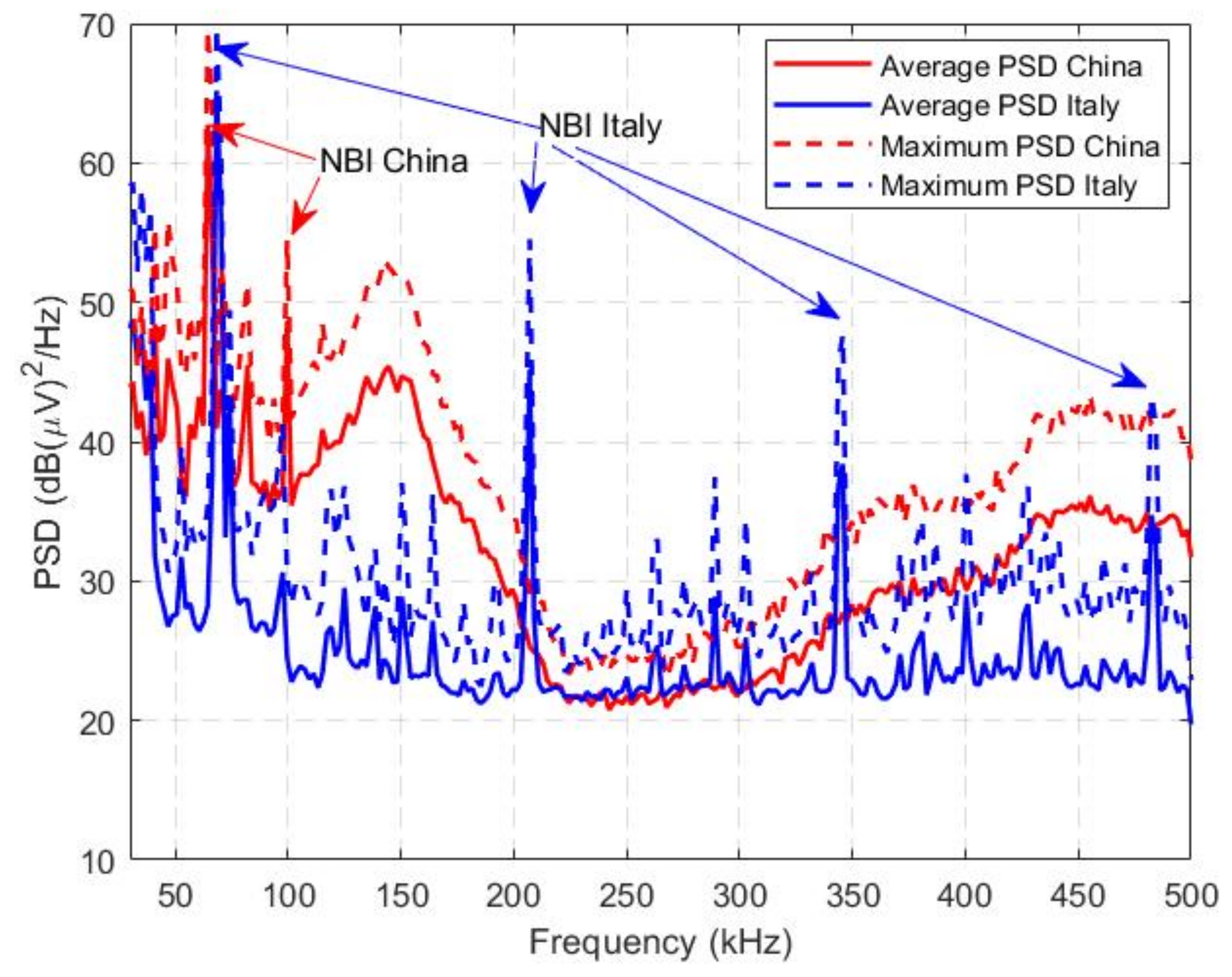
3.1. Power Spectrum Density Analysis

The PSD was calculated using the Welch method [32], using a Hanning window, averaging the frequency content over a long observation time of one mains period (20 ms). As shown in Figure 4, it can be observed that the average noise level in China is roughly 10–15 dB ${\left(\mu V\right)}^2/Hz$ higher than the one in Italy, while they are at the similar level of around 22 dB ${\left(\mu V\right)}^2/Hz$ in the range of 220–320 kHz. To some extent, noise measured in Italy can be regarded as white noise when frequency band is higher than 50 kHz, ignoring the effects of NBI.

According to EN 50065-1 [33], the measured transmitted signal shall not exceed 122 dB$\mu V$ with a peak detector with 200 Hz bandwidth from 95 kHz to 148.5 kHz. Besides, the voltage level of the transmitted signal can also refer to the measurement presented in [34], which was measured as 117 dB $\mathit{\mu }\mathit{V}$ in a lab environment in the frequency range of 95–135 kHz. The average noise PSD in Italy in the range of 95–148.5 kHz presented in Figure 4 (of around 25 dB ${\left(\mu V\right)}^2/Hz$), can be expressed as a noise level of 64.7 dB $\mu V$ taking into account a resolution bandwidth of 200 Hz, and the measurement impedance of 50 $\mathsf{\Omega }$. The noise level at the frequency of 270 kHz measured in China and Italy presented in Figure 4 (corresponding to 22 dB ${\left(\mu V\right)}^2/Hz$ ), can be calculated as 68.7 dB $\mu V$ with the resolution bandwidth of 1 kHz, and it is comparable with the noise floor level of around 60 dB $\mu V$ measured at 270 kHz with the resolution bandwidth of 1 kHz under line impedance stabilization network (50 $\mathsf{\Omega }$ output impedance) and presented in [35].

In narrowband PLC, NBI is usually caused by the loads connected in the network and its bandwidth is of less than 5 kHz. This case is completely different from what happens in broadband PLC, where NBI is often caused by radio waves with bandwidth of around 75 kHz. The PSD analysis shows that NBIs occur with the central frequency of 64.45 kHz and 99.61 kHz in noise measured in China, while they occur around 68.36 kHz, 207 kHz, 345.7 kHz, and 482 kHz, the odd multiples of 68.36 kHz. In these cases, the bandwidth of NBI is lower than 8 kHz.

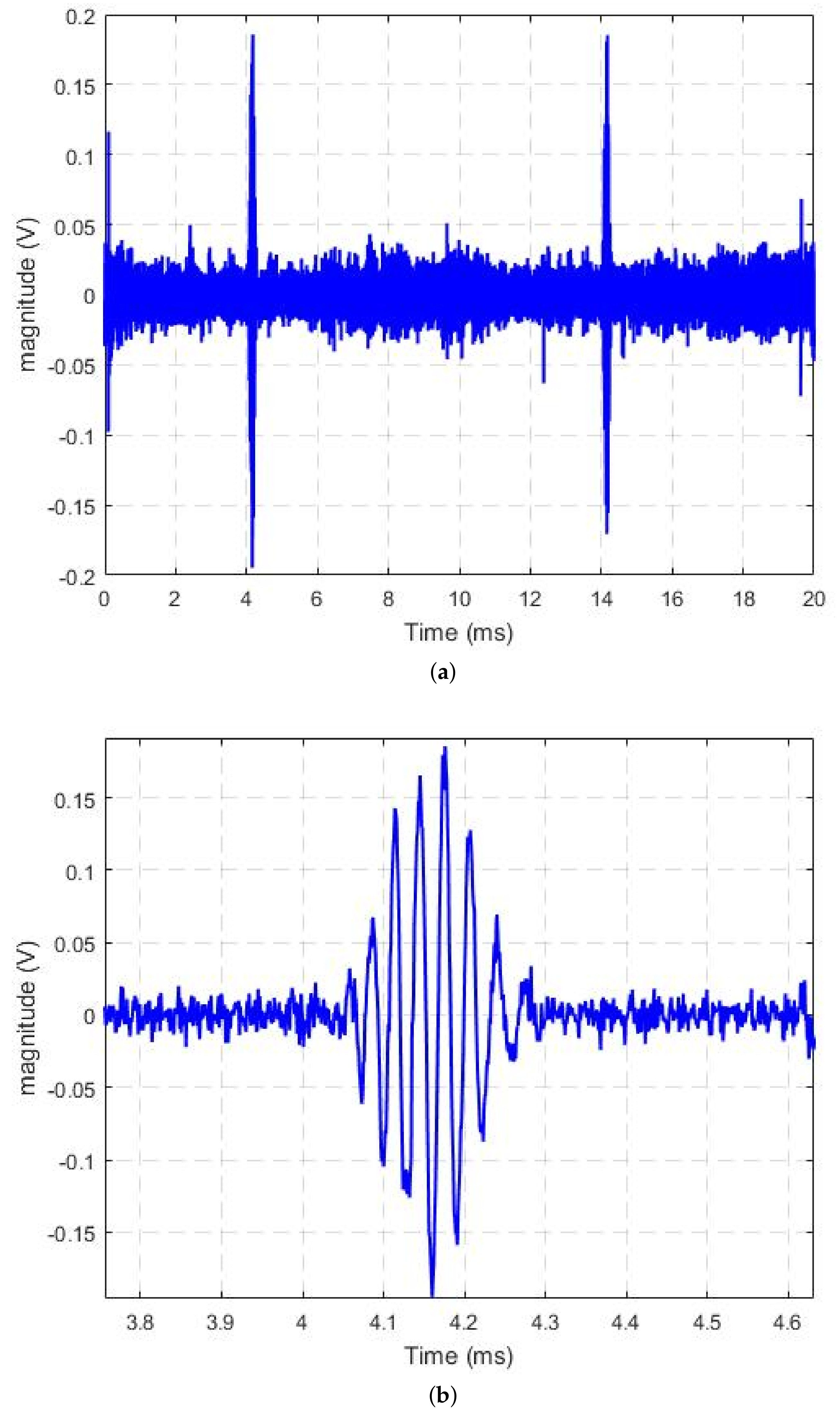
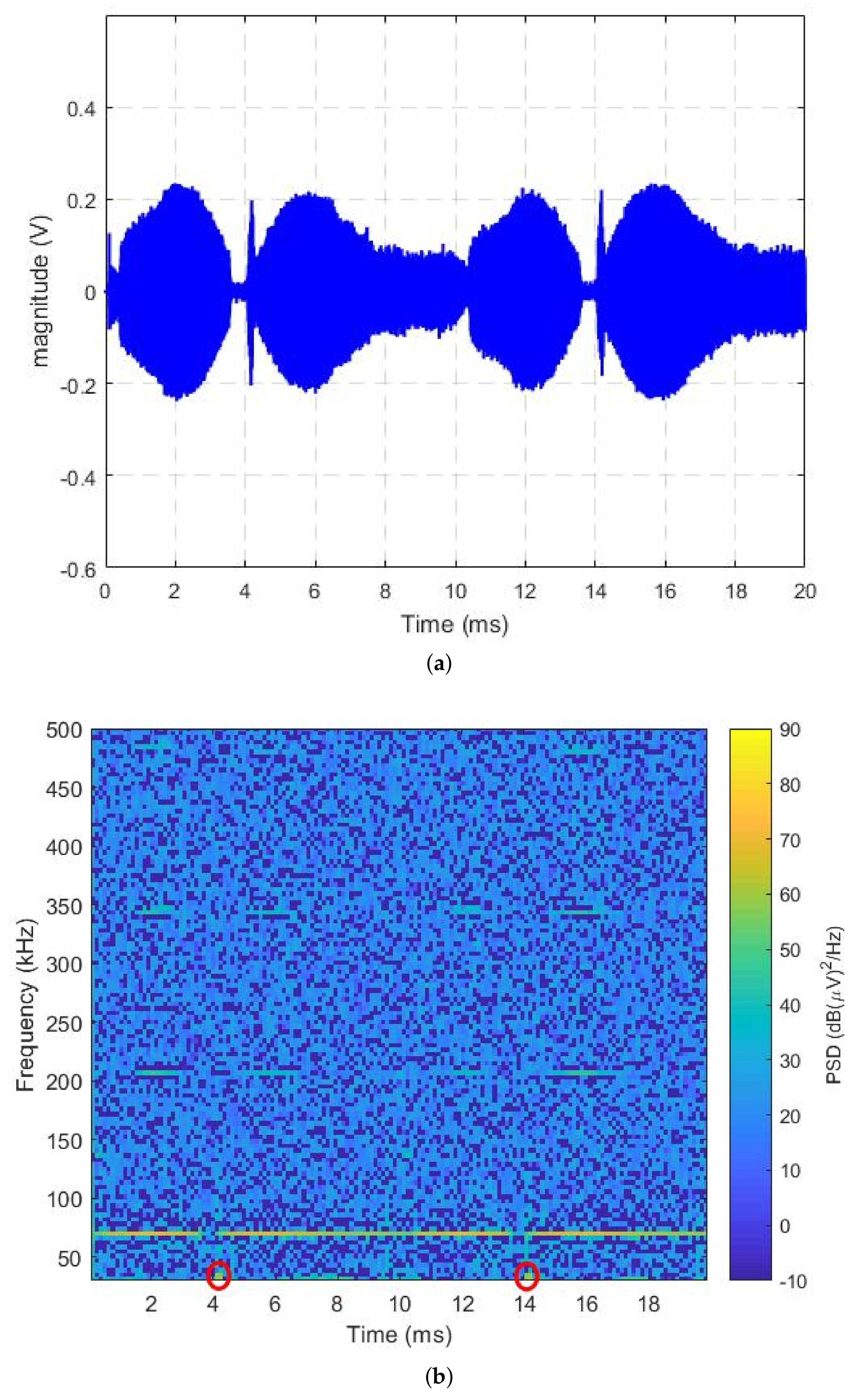
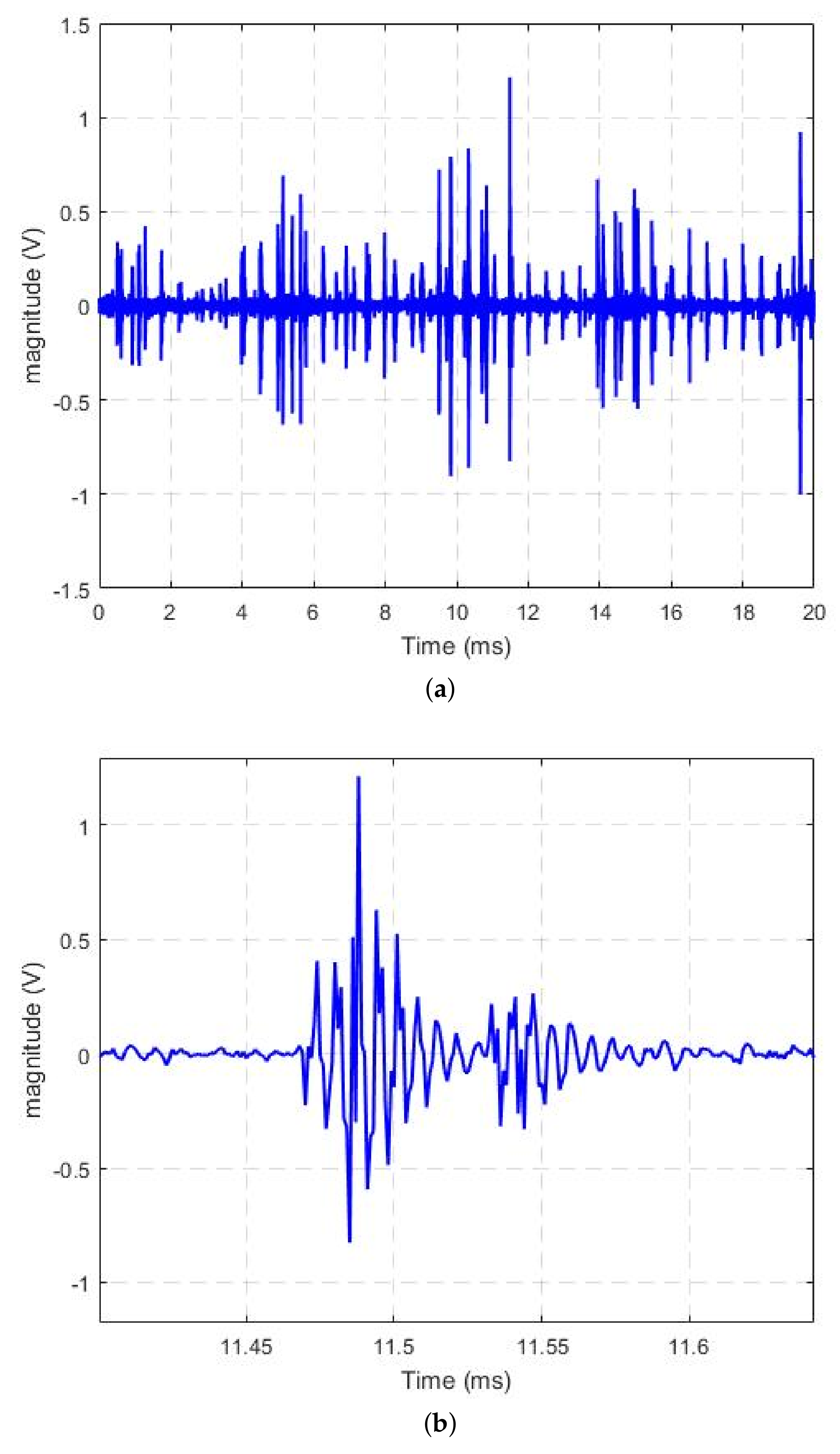
3.2. Time-Frequency Analysis

Narrowband PLC noise in general shows cyclostationary behavior [23]. We calculated the spectrogram of the noise by means of the STFT, by using a Hanning window of length 128 $\mu s$ (256 points FFT), and 50% overlap. In both Figure 5 and Figure 6, the cyclostationary behavior of the noise, synchronous with the 100Hz, can be clearly observed.

NBI measured in China always exists in the frequency of 64.45 kHz and 99.61 kHz in Figure 5b. PSD near 150 kHz and 450 kHz with wider frequency band remains high all the time, which can be seen as impulsive noise. Correspondingly, in Figure 5a impulsive noise occurs frequently in the whole time window, and even in the time window of 2–4 ms, the noise amplitude is lower but impulsive noise is still present, as it can be observed from the PSD near 450 kHz with frequency range of around 100 kHz in Figure 5b.

NBI measured in Italy in Figure 6 lower than 100 kHz occurs all the time, while its odd harmonics only occur in short time duration. It can be clearly seen that noise measured in Italy can be regarded as completely white noise without consideration of NBI. In Figure 6a, the magnitude of noise increases suddenly near 4 ms, and correspondingly, it displays higher power spectrum near 30 kHz with bandwidth around 15 kHz that is marked in red circles in Figure 6b, which also can be clearly seen in Figure 4.

It turns out that noise measured in China is full of impulsive noise all the time, while noise measured in Italy has hardly any impulsive noise but several NBIs. Impulsive noise is mainly caused by switching operations from both the mains system and electrical devices. The power quality of the mains system in both countries could be different, and thus different impulsive noise could be generated. The loads may contain some electronic devices such as AC/DC converters, which gives rise to impulsive noises. The devices in the measurements for both countries are manufactured by different producers and used in a different mains system, which could lead to different impulsive noise scenarios.

It is worth mentioning that NBI bandwidth is lower than 10 kHz, while sometimes impulsive noise only occupies around 20 kHz bandwidth in narrowband PLC. For this reason, when the noise bandwidth is near to 20 kHz, it is hard to differentiate between NBI and impulsive noise only in the frequency domain.

4. Impulsive Noise Modeling

As a result from the previous basic noise characteristic analysis, both in time and frequency domain, we can say that impulsive noise is not negligible in both countries, especially in China. In this section, two kinds of impulsive noise models are applied to reproduce the measured results. Before modeling, the noise data are preprocessed by eliminating NBIs in the frequency domain, because the bandwidth is too narrow to design a low order finite impulsive response filter. The noise wave in Figure 5a and Figure 6a are filtered, as shown in Figure 7 and Figure 8. After removing the NBI, the difference between the impulsive noise in the two countries is even more evident: the amplitude of impulsive noise in China goes up to 1.2 V; on the contrary it is lower than 0.2 V in Italy.

Figure 7 displays that noise measured in China is characterized by frequent impulses of short time duration, while Figure 8 shows that impulsive noise with longer time duration occurs only twice per mains period in Italy, which means that the frequency band occupation of IN will be narrow, around 15 kHz, located at the center frequency lower than 50 kHz. In fact, all the noise measured in Italy with different loads connected in the network are as shown in Figure 8. All the measured noise in China has similar noise wave shown in Figure 7, but the impulsive noise occurrences vary from load to load.

4.1. Model Methods

4.1.1. Middleton Class-A Model

The middleton class A model is composed of two terms as

$$N\left(t\right)=N_G\left(t\right)+N_I\left(t\right)=N_G\left(t\right)+\sum _i^{}{U}_j(t,\sigma ),$$

(1)

where $N_G\left(t\right)$ is a stationary Gaussian noise and $U_j$ represents the j-th impulsive noise wave. The PDF of $N\left(t\right)$ can be expressed as a mixture of zero-mean Gaussian terms weighted by a Poisson process,

$$f_N\left(n\right)=\sum _{m=0}^{\infty }{p}_m\frac{1}{\sqrt{2\pi {\delta }_m^2}}{e}^{\frac{-n^2}{2{\delta }_m^2}},with{p}_m=\frac{e^{-A}{A}^m}{m!},$$

(2)

where the variances ${\delta }_m^2$ can be expressed as

$${\delta }_m^2={\delta }_I^2\frac{m}{A}+{\delta }_G^2={\delta }_G^2(\frac{m}{A\mathsf{\Gamma }}+1)$$

(3)

in which ${\delta }_G^2$ is the variance of $N_G\left(t\right)$, ${\delta }_I^2$ denotes the variance of impulsive noise $N_I\left(t\right)$, $\mathsf{\Gamma }={\delta }_G^2/{\delta }_I^2$, and A is the impulse index, representing the density of impulses in one observed period. When building an MCA model, (2) will be truncated into M finite mixtures of Gaussian noise, yielding

$$\widetilde{f_N}\left(n\right)=\sum _{m=0}^{M-1}{p}_m^{{}^{\prime }}\frac{1}{\sqrt{2\pi {\delta }_m^2}}{e}^{\frac{-n^2}{2{\delta }_m^2}},with{p}_m^{{}^{\prime }}=\frac{p_m}{{\sum }_{m=0}^{M-1}{p}_m}.$$

(4)

4.1.2. $\alpha$-Stable Model

The $\alpha$-stable distribution shows a slow tail decay; for this reason, the $\alpha$-stable distribution tends to generate large-amplitude excursions which can be used to describe impulsive noise. It does not have a closed expression of PDF but offers a characteristic function, consequently the PDF can be derived by the inverse fast Fourier transform (IFFT) of the characteristic function. The characteristic function ${\mathsf{\Phi }}_X\left(\theta \right)$ of an $\alpha$-stable variable X can be expressed as

$${\mathsf{\Phi }}_X\left(\theta \right)=\left\{\begin{array}{c}exp\{j\mu \theta -{\sigma }^{\alpha }|\theta {|}^{\alpha }(1+j\beta sign\left(\theta \right)tan\left(\frac{\pi \alpha }{2}\right))\}\alpha \ne 1\hfill \\ exp\{j\mu \theta -\sigma |\theta \left|\right(1-j\beta \frac{2}{\pi }sign\left(\theta \right)ln\left|\theta \right|\left)\right\}\alpha =1\hfill \end{array}\right.$$

(5)

where $\theta \in \Re$ and

$$sign\left(\theta \right)=\left\{\begin{array}{c}1if\theta >0\hfill \\ 0if\theta =0\hfill \\ -1if\theta <0\hfill \end{array}\right.$$

(6)

In the above equations, there are four parameters: $\alpha$ is an index of stability when $0<\alpha <2$, the scale parameter $\delta$ ($\delta >0$), the skewness parameter $\beta$ ($-1<\beta <1$) and shift parameter $\mu$ ($\mu \in \Re$). If $\beta =0$, the variable X will follow a symmetrical $\alpha$ stable distribution about $\mu$, referred as $S\alpha S$. As a matter of fact, $\beta$ can be used as a measure of the asymmetry.

4.2. Results of Impulsive Noise Modeling

The process of modeling the impulsive noise mainly concentrates on obtaining the parameters of each model to characterize the measured noise. In both models, maximum likelihood estimation (MLE) is applied for the parameters estimation.

4.2.1. Middleton Class A model

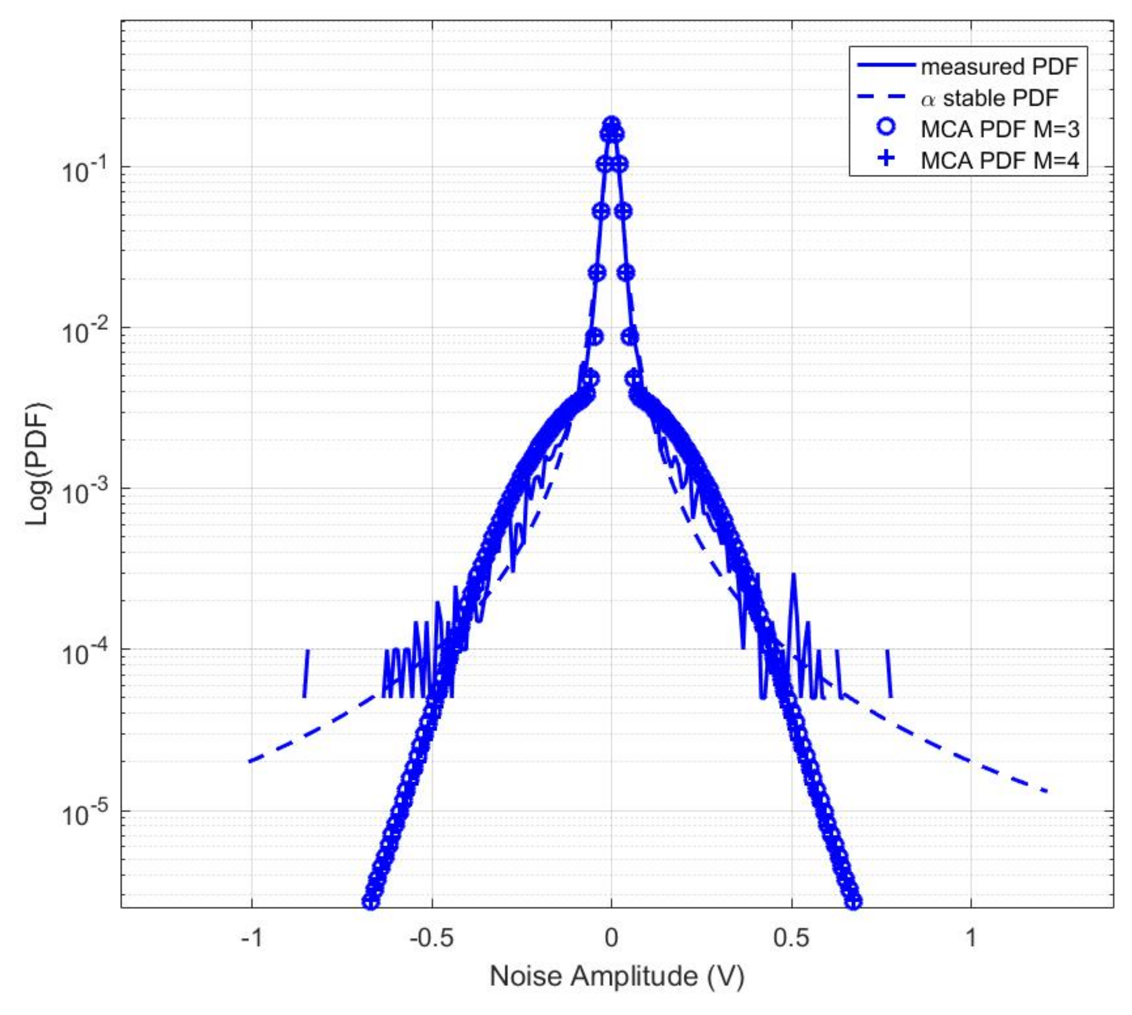
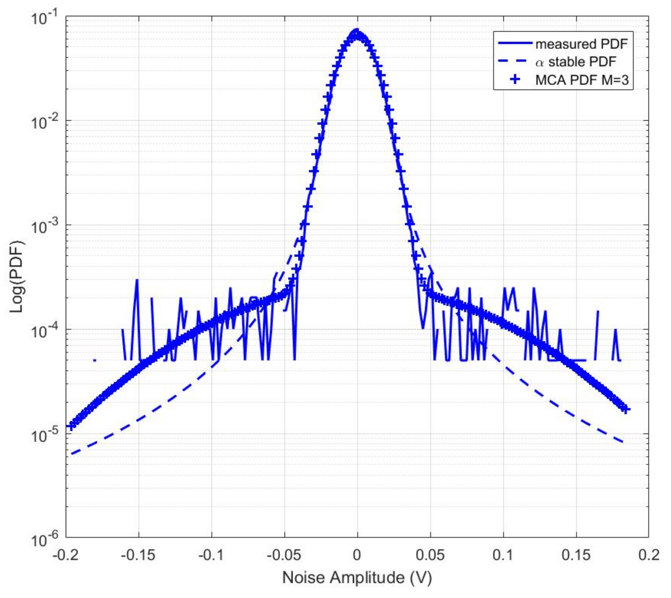
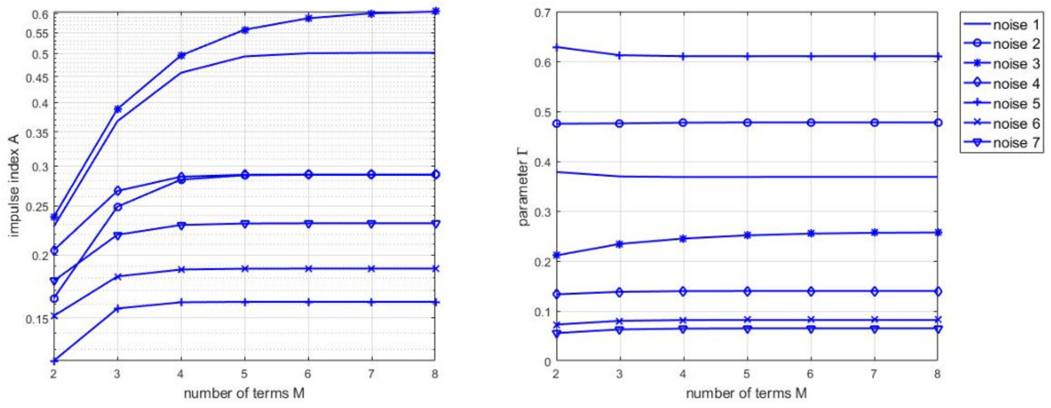
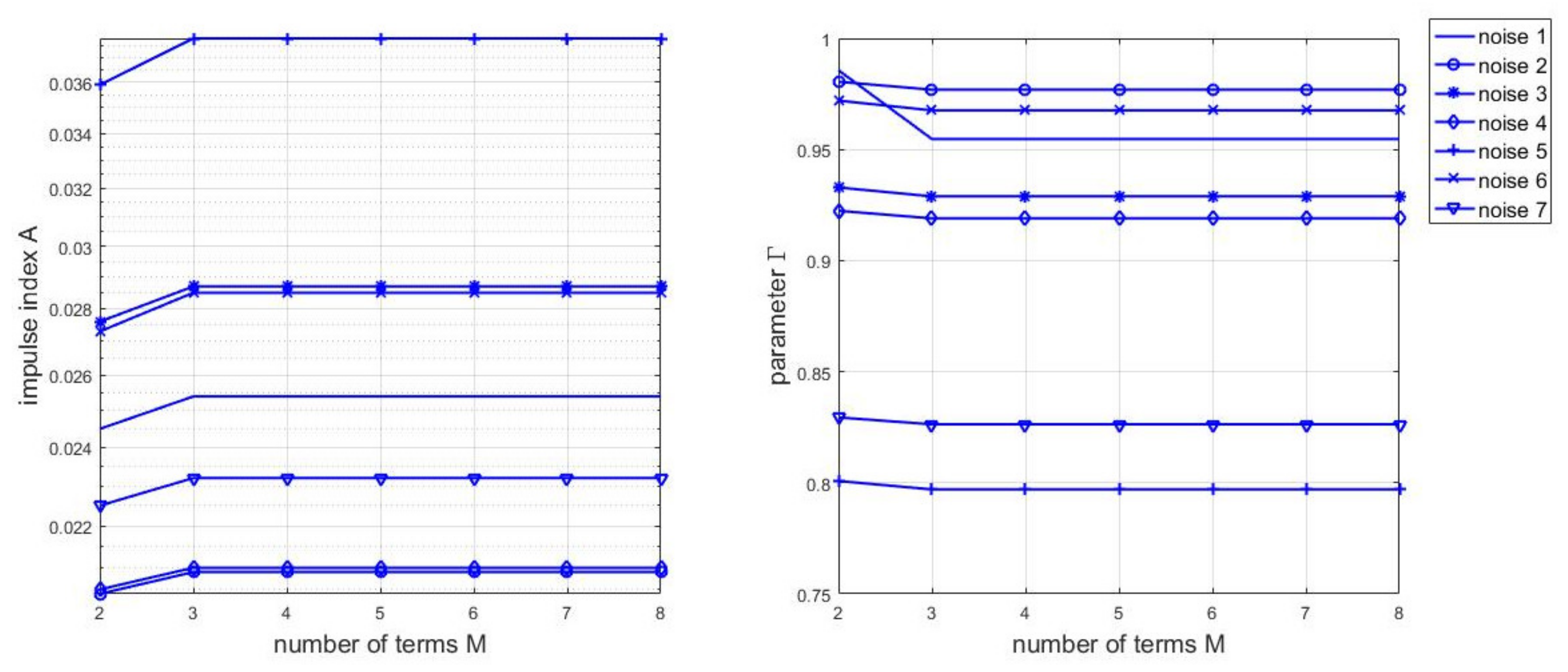
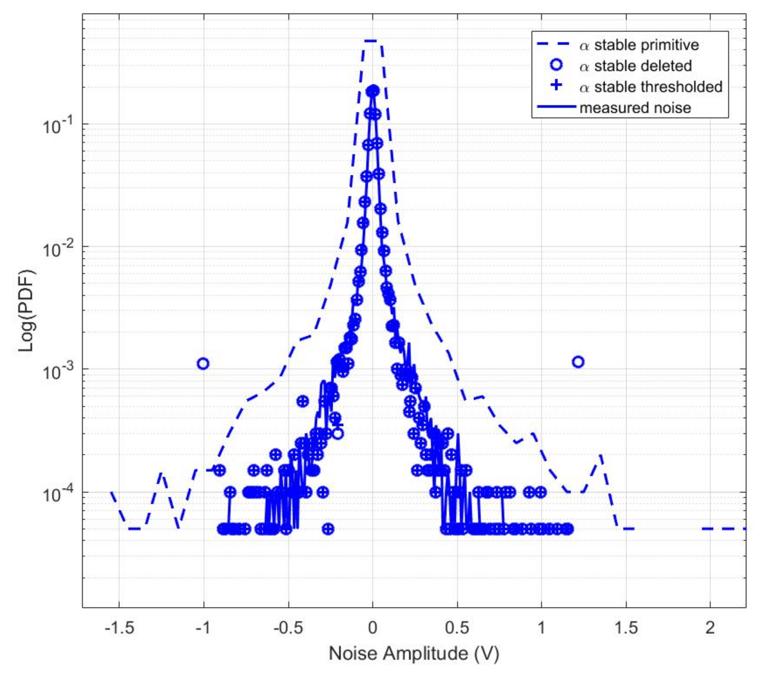
In the MCA model, three parameters must be estimated. The variance ${\delta }_G^2$ is derived from the background noise without impulsive noise, and the other two parameters A and $\mathsf{\Gamma }$ are estimated using MLE. The impulsive noise term M is selected when the maximum likelihood reaches a steady value considering different noises measured with different loads. Figure 9 and Figure 10 show seven different noises (measured when different loads are connected) in China and Italy, respectively. It is evident that when M is larger than 3, most of the parameters remain unchanged. Therefore, M is considered equal to 3, which is also proposed in [36].

From Figure 9, it can be noted that impulse index A in the noise measured in China is over 0.16, while it is lower than 0.04 in Figure 10. In addition, parameter $\mathsf{\Gamma }$ is less than 0.7 in China, conversely, and it is higher than 0.75 in Italy, implying that the average background noise power is smaller in the whole noise power in China while, on the contrary, power line channel in China is greatly interfered by impulsive noise.

4.2.2. $\alpha$ Stable Distribution Model

All four parameters in $\alpha$ stable distribution model are estimated by using MLE. In

Table 2. The parameters estimation of $\alpha$ stable distribution of noise in China.

Noise	$\mathit{\alpha }$	$\mathit{\beta }$	$\mathit{\delta }$	$\mathit{\mu }$
noise 1	1.59264	−0.00636769	0.0189837	7.06 × 10${}^{-6}$
noise 2	1.56769	−0.0165415	0.016261	9.62 × 10${}^{-5}$
noise 3	1.63601	−0.0257861	0.0212625	2.10 × 10${}^{-4}$
noise 4	1.25285	−0.00828737	0.0165645	3.28 × 10${}^{-5}$
noise 5	1.43699	−0.00552512	0.012531	9.54 × 10${}^{-6}$
noise 6	1.21431	−0.0104543	0.0148703	7.41 × 10${}^{-5}$
noise 7	1.18904	−0.00616141	0.0165906	3.46 × 10${}^{-5}$

, all the noise in China that has been previously modeled by MCA are examined also in this case. In the $\alpha$ stable distribution, when $\alpha =2$, the distribution will reduce to the Gaussian distribution; when $\alpha <2$, the distribution shows heavy tails that can be used to model the impulsive noise. Table 2 shows that $\beta$ is close to zero, meaning that noise waves are almost zero symmetrical, as the mean value $\mu$ is rather close to zero as well. For noise measured in Italy, as shown in

Table 3. The parameters estimation of $\alpha$ stable distribution of noise in Italy.

Noise	$\mathit{\alpha }$	$\mathit{\beta }$	$\mathit{\delta }$	$\mathit{\mu }$
noise 1	1.75966	0.0282014	0.00760994	−3.33 × 10${}^{-5}$
noise 2	1.78562	0.00118321	0.0078767	1.21 × 10${}^{-5}$
noise 3	1.75686	0.0565987	0.00792512	−1.16 × 10${}^{-4}$
noise 4	1.7938	−0.0211009	0.00790263	3.57 × 10${}^{-5}$
noise 5	1.74286	0.0265969	0.00835163	−6.45 × 10${}^{-5}$
noise 6	1.77606	−0.0156829	0.00890917	2.53 × 10${}^{-5}$
noise 7	1.85054	−0.022285	0.0108844	4.48 × 10${}^{-5}$

, a similar conclusion can be reached that the noise is symmetrical with zero mean. Therefore, the model can be viewed as $S\alpha S$ distribution. Comparing $\alpha$ in Table 2 and Table 3, $\alpha$ of the noise in China is lower than the one in Italy; this corresponds to the previous frequency/time domain analysis in which we understood that power line channels in China are highly interfered by impulsive noise and $\alpha$ of noise in China varies greatly from load to load, while that of noise in Italy varies slightly.

In Figure 11, it is shown that in the lower range of noise amplitude, both models can characterize impulsive noise well, while with the increase of the absolute of amplitude, it is noted that $\alpha$ stable distribution models are better than the MCA model. In Figure 12, with lower amplitude of noise measured in Italy, both models fit the measured noise well. When the amplitude increases, it shows that MCA model fits the tendency of impulsive noise better.

The primitive MCA model consists of infinite terms, and is truncated into finite terms when modeling, thus the noise generated based on the MCA model will be limited in a reasonable range determined by the parameters A and $\mathsf{\Gamma }$. However, due to the asymptotic behavior of $\alpha$ stable distribution, the variance of stable distribution is infinite for $0<\alpha <2$. The amplitude of the noise generated by $\alpha$ stable distribution varies in a relatively large range, far exceeding the measured noise. From what we have discussed above, it is possible to draw the conclusion that $\alpha$ stable distribution fits noise measured in China better, while MCA model fits noise measured in Italy better. Therefore, when $\alpha$ stable distribution is applied to generate noise, the amplitude of the noise has to be restricted into a reasonable range. There are two ways to limit the generated noise, one is thresholding, and the other is deleting. In the former method of thresholding, thresholded noise $N_{th}\left(n\right)$ can be expressed as

$$N_{th}\left(n\right)=\left\{\begin{array}{c}{N}_{\alpha }\left(n\right)if\left|N_{\alpha }\left(n\right)\right|<T\hfill \\ T\ast sgn\left(N_{\alpha }\left(n\right)\right)otherwise\hfill \end{array}\right.$$

(7)

where $sgn\left(\right)$ denotes sign function, $N_{\alpha }\left(n\right)$ denotes noise generated by $\alpha$ stable distribution directly, and T is the threshold. In the latter method of deleting, if the noise sample is over the threshold, it will be abandoned. To compare the performance of noise generation based on $\alpha$ stable distribution, $Log$(PDF) of the primitive noise generated by $\alpha$ stable distribution, the deleted one, the thresholded one and the measured noise are compared, as shown in Figure 13. We can see that with noise preprocessing, PDF fits well with the measured noise. Further, two methods of preprocessing originally generated noise make no difference and both fit well. Therefore, both thresholding and deleting methods can be adopted for generating impulsive noise.

5. Conclusions

In this paper, noise measured in China and Italy of 30–500 kHz are compared based on basic characteristics in frequency and time domain using PSD and STFT. It is proved that noise measured in China is characterized by higher noise level in the whole frequency band, while the noise measured in Italy only has higher PSD in frequency lower than 50 kHz, and can be regarded as white noise in the frequency band higher than 50 kHz without considering NBI. Impulsive noise models are further built using MCA and $\alpha$ stable distribution model. The results show that noise measured in China can be fitted better by $\alpha$ stable distribution model, while noise measured in Italy can be modeled better based on MCA. In summary, power line channels in China are far more hostile than those in Italy due to high noise interferences.

References

1. Ferreira, H.C.; Grove, H.M.; Hooijen, O.; Han Vinck, A.J. Power line communications: An overview. In Proceedings of the IEEE AFRICON 4th AFRICON, Stellenbosch, South Africa, 27 September 1996; Volume 9, pp. 142–149. [Google Scholar]
2. Cano, C.; Pittolo, A.; Malone, D.; Lampe, L.; Tonello, A.M.; Dabak, A.G. State of the Art in Power Line Communications: From the Applications to the Medium. IEEE J. Sel. Areas Commun. 2016, 7, 1935–1952. [Google Scholar] [CrossRef]
3. Gu, Z.; Liu, H.; Liu, D.; Man, K.L.; Liang, H. Modeling the Noise in NarrowBand Power Line Communication. Int. J. Control Autom. 2016, 2, 41–48. [Google Scholar] [CrossRef]
4. Pereira, S.C.; Caporali, A.S.; Casella, I.R.S. Power line communication technology in industrial network. In Proceedings of the 2015 International Symposium on Power Line Communications and its Applications (ISPLC), Austin, TX, USA, 29 March–1 April 2015; Volume 7. [Google Scholar]
5. O’Neal, J.B. The Residential Power Circuit as a Communication Medium. IEEE Trans. Consum. Electron. 1986, 8, 567–577. [Google Scholar] [CrossRef]
6. Vines, R.M.; Joel Trissell, H.; Gale, L.J.; O’neal, J.B. Noise on Residential Power Distribution Circuits. IEEE Trans. Electromagn. Compat. 1984, 11, 161–168. [Google Scholar] [CrossRef]
7. Cooper, D.; Jeans, T. Narrowband, low data rate communications on the low-voltage mains in the CENELEC frequencies. I. Noise and attenuation. IEEE Trans. Power Deliv. 2012, 7, 718–723. [Google Scholar] [CrossRef]
8. IEEE Standard on Channel and Noise Measurements; P1901.2; IEEE: New York, NY, USA, 2011.
9. Emleh, A.; de Beer, A.S.; Ferreira, H.C.; Han Vinck, A.J. Noise generated by modern lamps and the influence on the smart-grid communication network. In Proceedings of the 2015 IEEE International Conference on Smart Grid Communications (SmartGridComm), Miami, FL, USA, 2–5 November 2015; Volume 3. [Google Scholar]
10. Dalichau, H.; Täger, W. Description of the technology and comparison of the performance of two different approaches for a powerline modem in the Cenelec-band. In Proceedings of the 4 th International Symposium on Powerline Communications, Limerick, Ireland, 5–7 April 2000; Volume 4. [Google Scholar]
11. Gassara, H.; Rouissi, F.; Ghazel, A. Narrowband stationary noise characterization and modelling for power line communication. In Proceedings of the 13th International Symposium on Communications and Information Technologies (ISCIT), Surat Thani, Thailand, 4–6 September 2013; Volume 10. [Google Scholar]
12. Gassara, H.; Rouissi, F.; Ghazel, A. A Novel Stochastic Model for the Impulsive Noise in the Narrowband Indoor PLC Environment. In Proceedings of the 2015 IEEE International Instrumentation and Measurement Technology Conference (I2MTC), Pisa, Italy, 11–14 May 2015; Volume 7. [Google Scholar]
13. Hagmann, W. A spread spectrum communication system for load management and distribution automation. IEEE Trans. Power Deliv. 1989, 1, 75–81. [Google Scholar] [CrossRef]
14. Tanaka, M. High frequency noise power spectrum, impedance and transmission loss of power line in Japan on intrabuilding power line communications. IEEE Trans. Consum. Electron. 1988, 5, 321–326. [Google Scholar] [CrossRef]
15. Lasciandare, A.; Garotta, S.; Veroni, F.; Saccani, E.; Guerrieri, L.; Arrigo, D. Experimental field trials of a utility AMR power line communication system analyzing channel effects and error correction methods. In Proceedings of the IEEE International Symposium on Power Line Communications and Its Applications, Pisa, Italy, 26–28 March 2007; Volume 6. [Google Scholar]
16. Zimmermann, M.; Dostert, K. Analysis and Modeling of Impulsive Noise in Broad-Band Powerline Communications. IEEE Trans. Electromagn. Compat. 2002, 7, 249–258. [Google Scholar] [CrossRef]
17. Han, B.; Stoica, V.; Kaiser, C.; Otterbach, N.; Dostert, K. Noise characterization and emulation for low-voltage power line channels across narrowband and broadband. Digit. Signal Process. 2017, 69, 259–274. [Google Scholar] [CrossRef]
18. Meng, H.; Guan, Y.L.; Chen, S. Modeling and analysis of noise effects on broadband power-line communications. IEEE Trans. Power Deliv. 2005, 4, 630–637. [Google Scholar] [CrossRef]
19. Andreadou, N.; Pavlidou, F.N. Modeling the Noise on the OFDM Power-Line Communications System. IEEE Trans. Power Deliv. 2009, 12, 150–157. [Google Scholar] [CrossRef]
20. Bauer, M.; Liu, W.Q.; Dostert, K. Channel emulation of low-speed PLC transmission channels. In Proceedings of the IEEE International Symposium on Power Line Communications and Its Applications (ISPLC), Dresden, Germany, 29 March–1 April 2009; Volume 5. [Google Scholar]
21. Nieman, K.F.; Lin, J.; Nassar, M.; Waheed, K.; Evans, B.L. Cyclic spectral analysis of power line noise in the 3–200 kHz band. In Proceedings of the IEEE International Symposium on Power Line Communications and Its Applications (ISPLC), Johannesburg, South Africa, 24–27 March 2013; Volume 6. [Google Scholar]
22. Kaiser, C.; Otterbach, N.; Dostert, K. Spectral correlation analysis of narrowband power line noise. In Proceedings of the IEEE International Symposium on Power Line Communications and its Applications (ISPLC), Madrid, Spain, 3–5 April 2017; Volume 4. [Google Scholar]
23. Nassar, M.; Dabak, A.; Kim, H., II; Pande, T.; Evans, B.L. Cyclostationary noise modeling in narrowband powerline communication for Smart Grid applications. In Proceedings of the 2012 IEEE International Conference on Acoustics, Speech and Signal Processing (ICASSP), Kyoto, Japan, 25–30 March 2012; Volume 8. [Google Scholar]
24. Middleton, D. Statistical-Physical Models of Electromagnetic Interference. IEEE Trans. Electromagn. Compat. 1977, 8, 106–127. [Google Scholar] [CrossRef]
25. Ndo, G.; Labeau, F.; Kassouf, M. A Markov-Middleton Model for Bursty Impulsive Noise: Modeling and Receiver Design. IEEE Trans. Power Deliv. 2013, 8, 2317–2325. [Google Scholar] [CrossRef]
26. Rouissi, F.; Han Vinck, A.J.; Gassara, H.; Ghazel, A. Statistical characterization and modelling of impulse noise on indoor narrowband PLC environment. In Proceedings of the 2017 IEEE International Symposium on Power Line Communications and its Applications (ISPLC), Madrid, Spain, 3–5 April 2017; Volume 4. [Google Scholar]
27. Shao, M.; Nikias, C.L. Signal processing with fractional lower order moments: stable processes and their applications. Proc. IEEE 1993, 7, 986–1010. [Google Scholar] [CrossRef]
28. Tran, T.H.; Do, D.D.; Huynh, T.H. PLC Impulsive Noise in Industrial Zone: Measurement and Characterization. Int. J. Comput. Electr. Eng. 2013, 2, 48–51. [Google Scholar] [CrossRef]
29. Laguna-Sanchez, G.; Lopez-Guerrero, M. An experimental study of the effect of human activity on the alpha-stable characteristics of the power-line noise. In Proceedings of the IEEE International Symposium on Power Line Communications and its Applications (ISPLC), Glasgow, UK, 30 March–2 April 2014; Volume 5. [Google Scholar]
30. Laguna-Sanchez, G.; Lopez-Guerrero, M. On the Use of Alpha-Stable Distributions in Noise Modeling for PLC. IEEE Trans. Power Deliv. 2015, 1, 1863–1870. [Google Scholar] [CrossRef]
31. Gassara, H.; Chaker Bali, M.; Duval, F.; Rouissi, F.; Ghazel, A. Coupling interface circuit design for experimental characterization of the narrowband power line communication channel. In Proceedings of the IEEE International Symposium onElectromagnetic Compatibility (EMC), Pittsburgh, PA, USA, 6–10 August 2012; Volume 8. [Google Scholar]
32. Welch, P. The use of fast Fourier transform for the estimation of power spectra: A method based on time averaging over short, modified periodograms. IEEE Trans. Audio Electroacoust. 1967, 6, 70–73. [Google Scholar] [CrossRef]
33. Standard CENELEC. EN 50065-1:2012. Signaling in Low-Voltage Electrical Installations in the Frequency Range 3 kHz– 148. 5 kHz- Part 1: General Requirements Frequency Bands and Electromagnetic Disturbances; European Committee for Electrotechnical Standardization: Brussels, Belgium, 2011; Volume 4. [Google Scholar]
34. Artale, G.; Cataliotti, A.; Cosentino, V.; Di Cara, D.; and Fiorelli, R.; Guaiana, S.; Tine, G. A New Low Cost Coupling System for Power Line Communication on Medium Voltage Smart grids. IEEE Trans. Smart Grid 2016, PP, 1. [Google Scholar] [CrossRef]
35. Mishra, A.; Tayal, H.; Khan, M.A.; Raza, M. Suitable PHY layer of narrow-band power line carrier communication in emerging advanced metering infrastructure scenario. In Proceedings of the 2015 IEEE Conference on Standards for Communications and Networking (CSCN), Tokyo, Japan, 28–30 October 2015; Volume 10. [Google Scholar]
36. Cortés, J.A.; Sanz, A.; Estopiñán, P.; García, J.I. On the suitability of the Middleton class A noise model for narrowband PLC. In Proceedings of the International Symposium on Power Line Communications and its Applications (ISPLC), Bottrop, Germany, 20–23 March 2016; Volume 5. [Google Scholar]
Figure 1. Measurement setup for noise collection.
Energies 11 00863 g001
Figure 2. Coupling filter circuit.
Energies 11 00863 g002
Figure 3. Transfer function of the coupling filter.
Energies 11 00863 g003
Figure 4. Noise PSD comparison between China and Italy.
Energies 11 00863 g004
Figure 5. Noise measured in China (a) noise wave; (b) noise spectrogram .
Energies 11 00863 g005
Figure 6. Noise measured in Italy (a) noise wave; (b) noise spectrogram .
Energies 11 00863 g006
Figure 7. Noise measured in China without NBI (a) 20 ms time windwow; (b) short time window.
Energies 11 00863 g007
Figure 8. Noise measured in Italy without NBI (a) 20 ms time windwow; (b) short time window.
Energies 11 00863 g008
Figure 9. A and Γ versus the number of terms M for noise measured in China.
Energies 11 00863 g009
Figure 10. A and Γ versus the number of terms M for noise measured in Italy.
Energies 11 00863 g010
Figure 11. log(PDF) comparison of MCA , α stable model and measured noise data in China.
Energies 11 00863 g011
Figure 12. log(PDF) comparison of MCA, α stable model and measured noise data in Italy.
Energies 11 00863 g012
Figure 13. log(PDF) comparison of α stable primitive noise, α stable thresholded noise and measured noise data in China.
Energies 11 00863 g013