Scheduling Appliances with GA, TLBO, FA, OSR and Their Hybrids Using Chance Constrained Optimization for Smart Homes


1
School of Electrical Engineering and Computer Science, National University of Sciences and Technology, Islamabad 44000, Pakistan
2
COMSATS Institute of Information Technology, Islamabad 44000, Pakistan
*
Author to whom correspondence should be addressed.
Energies 2018, 11(4), 888; https://doi.org/10.3390/en11040888
Submission received: 26 January 2018
/
Revised: 22 March 2018
/
Accepted: 2 April 2018
/
Published: 10 April 2018
(This article belongs to the Special Issue Energy Efficient and Smart Cities)
Abstract
:In this paper, we design a controller for home energy management based on following meta-heuristic algorithms: teaching learning-based optimization (TLBO), genetic algorithm (GA), firefly algorithm (FA) and optimal stopping rule (OSR) theory. The principal goal of designing this controller is to reduce the energy consumption of residential sectors while reducing consumer’s electricity bill and maximizing user comfort. Additionally, we propose three hybrid schemes OSR-GA, OSR-TLBO and OSR-FA, by combining the best features of existing algorithms. We have also optimized the desired parameters: peak to average ratio, energy consumption, cost, and user comfort (appliance waiting time) for 20, 50, 100 and 200 heterogeneous homes in two steps. In the first step, we obtain the optimal scheduling of home appliances implementing our aforementioned hybrid schemes for single and multiple homes while considering user preferences and threshold base policy. In the second step, we formulate our problem through chance constrained optimization. Simulation results show that proposed hybrid scheduling schemes outperformed for single and multiple homes and they shift the consumer load demand exceeding a predefined threshold to the hours where the electricity price is low thus following the threshold base policy. This helps to reduce electricity cost while considering the comfort of a user by minimizing delay and peak to average ratio. In addition, chance-constrained optimization is used to ensure the scheduling of appliances while considering the uncertainties of a load hence smoothing the load curtailment. The major focus is to keep the appliances power consumption within the power constraint, while keeping power consumption below a pre-defined acceptable level. Moreover, the feasible regions of appliances electricity consumption are calculated which show the relationship between cost and energy consumption and cost and waiting time.
1. Introduction
With an exponential rise in energy demand, accompanied by the continuous decline in energy generation, an ongoing up gradation is required in today’s energy infrastructure. Academia and research communities have considered it to be the serious concern for addressing future energy demands. The concept of smart electricity system has moved the conventional grid to the smart grid. The smart grid (SG) impersonates a perception of the future electric generation system integrated with advanced sensing technology, two-way communication at transmission and distribution level to efficiently supply smart electricity in a smart way. Reliability, cost saving, self-healing, self-optimization and consumer friendly pollutant reduction are few of the many benefits of the smart grid. The smart grid is motivated by several economic, social and environmental factors.
Demand-side management (DSM) is the modification of energy demand for the consumer in response to variation in electricity prices. DSM follows three steps; planning, implementing and monitoring activities of the utility particularly designed to give awareness to consumers to modify their level of using electricity. In literature, there are different DSM strategies proposed such as load shifting, valley filling, demand response, etc. By adopting these strategies consumers can shift their load from on-peak to off-peak hours. Demand response and load management are the key functions of DSM. Demand response is defined as changes in end-user electricity usage in response to the variation in electricity prices over time. The demand response programs include price-based and incentive-based demand response program. In incentive-based demand response, consumers are provided with some financial benefits, if they follow the instructions provided by the utility. In price-based demand response, consumers are offered with the time-varying pricing scheme. The consumer will adjust the schedule according to the dynamic pricing scheme.
The dynamic scheme includes extreme day pricing (EDP), critical peak pricing (CPP), day-ahead pricing (DAP), extreme day cpp (ED-CPP) and real time pricing (RTP) [1]. Both the consumer and utility get the benefit of these programs. On the consumer side, consumers get incentives by shifting their load to off-peak hours from on-peak hours in terms of reduction in expense of electricity bill. On the other hand, peak load reduction helps to improve the utility stability and reliability. Further, the advance monitoring infrastructure (AMI) along with the other devices has made it possible to get the usage data. With this data, the energy management controller provides the energy consumption schedule to the common user. A programmable logic controller (PLC) is then used to implement the proposed algorithm in order to provide an optimized solution and it also provides an interface between the controller, sensors, smart meter and the appliances. Moreover, PLCs provide modules which process signals that require specific interfacing requirements.
The smart grid community is actively participating in highlighting the various demand response problems. The research conducted in the US shows that about 42% of energy usage in the residential sector are consumed by household appliances. In [2], the operating time for all appliances is known and the appliance scheduling is considered for the assumed length of operational time. In [3], the authors study scheduling problem with the known energy consumption habits of a user. In [2,3], the authors considered a single home in order to find the energy optimization schedule. The authors consider multiple consumers with known energy consumption of all appliances in order to find optimal starting time of the appliances in [4]. In the proposed technique, the peak load is not reduced rather it is shifted to off-peak hours from on-peak hours. In [5], the stochastic algorithm is used to solve the distributed problem. In this paper, the energy consumption and length of operation is fixed along with the assumption that each appliance has its own flexible starting time whereas in [6], the starting and ending time of the appliance is considered along with the varied energy consumption. This problem is resolved by game theory approach and in this problem, users get their electricity bills based on their daily energy consumption schedule. In [7,8,9,10], non-integer linear programming (NILP), mixed integer linear programming (MILP), mixed integer nonlinear programming (MINLP) and convex programming are used for cost minimization and energy consumption scheduling. Moreover, these techniques are a predefined set of instructions that work well for small data set but fail to handle complex data set. Secondly, the computational cost of such algorithms is too high.
Along with this, we are exploiting different parameters of the meta-heuristic algorithm and mathematical algorithm optimal stopping rule (OSR) in order to find an optimal schedule for home appliances based on priority constraint. The opportunistic scheduling refers to the best starting time of the appliances based on their priority. Each appliance has its own priority and length of operational time. The appliance with high priority has high cost and lesser waiting time and vice versa. We can clearly see the trade-off between peak to average ratio (PAR) and electricity cost. The simulations are conducted on a single home and multiple homes (comprised of 20, 50, 100 and 200 homes). There are three categories of appliances: shift able appliances, unshiftable appliances and uninterrupted appliances. Non Shiftable appliances are considered as fixed or base classes they consume fix power consumption in any case. Uninterrupted appliances once started cannot be shifted to any other time slot. As scheduled, these appliances will not help us to achieve our desired objective so we will only consider shift-able appliances. The major objective of our work is electricity cost reduction and analyzing the impact of priority constraint waiting time and cost. Additionally, the yearly cost saving for appliances is also taken into account. Based on above-aforementioned objectives, the motives of our work are clearly highlighted and it shows that achieving our desired objectives is significant for both consumers and utility. By applying chance-constrained optimization, we remove the load uncertainty which helps to limit the power range of appliances.
The main motivation of our work is to tackle the major challenges faced by the conventional grid. These challenges vary from country to country according to their energy needs and requirements. In developing countries, energy needs are fulfilled by possible energy supply, or by providing direct access to the utility. On the other hand, the underdeveloped countries still face the problems associated with energy consumption management which disturbs the utility stability. Although in different countries, these circumstances vary based on their situations. In proposed work, we provide the cost-effective energy optimization solution for the residential home energy management in order to attain multiple objectives such as minimum cost and maximum user comfort which incentivizes both the utility as well as the regular consumer.
Generally, Demand response schemes work by shifting the load to off-peak hours from on-peak hours which minimizes the overall energy usage. The former motivates the consumer with price based and incentive-based schemes to restrain high peaks which help to maintain grid stability. However, load shifting may reduce the electricity bills and ultimately may disturb the consumer’s comfort. So, there is a trade-off between electricity cost and user comfort. Although the above-mentioned research study has explored the various aspects of residential home energy management. However, mostly their focus is on one of the objectives either on the cost minimization or the user comfort maximization. In this paper, we take both objectives into consideration minimum cost as well as maximum user comfort. Other than this, we proposed hybrid techniques population-based metaheuristic approaches OSR-GA, OSR-TLBO and OSR-FA. These techniques have easy computation, fast convergence and less operational time.
The major contributions of our work are:
- Proposed novel hybridization techniques: OSR-GA, OSR-TLBO and OSR-FA
- Simulation is done for the residential area which includes single home, 20, 50, 100 and 200 homes.
- Based on user-defined priority we calculate the yearly based cost minimization.
- We incorporate the threshold-based policy and chance constrained optimization (CCO) technique.
- Different performance parameters are tuned to find out the relation between cost and waiting time and cost and PAR.
- The feasible region of the appliances is calculated to find the relation between cost and energy consumption and cost and waiting time.
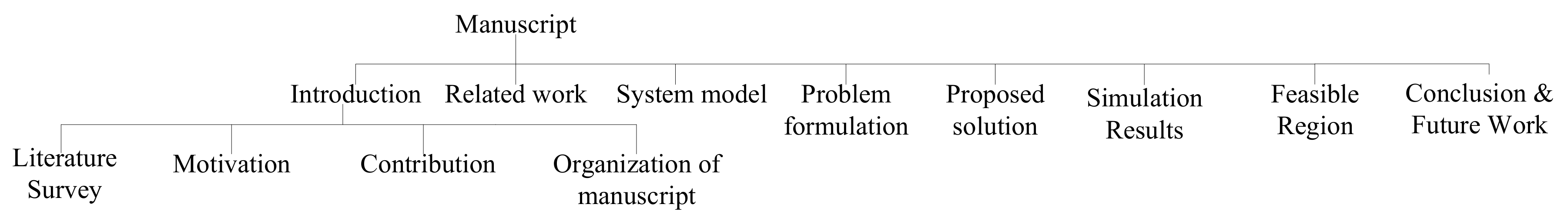
The paper is divided into six sections. The first section includes the introduction of the smart grid, the background knowledge, its significance, and the motivation behind the study. The remaining paper is composed in the following way. Section 2 covers the literature review where previous research in this domain has been critically analyzed to explore the new findings in this domain. Later on, this section is comprehended in the form of the table. Section 3 describes the system model. The problem description and formulation is elaborated in Section 4. The proposed solution their description and algorithms are organized in Section 5. The results of simulations and the performance comparison are shown in Section 6. The feasible reason is presented in Section 7 and at the end; the whole summary and the future work is concluded in Section 8. The schematic overview of this manuscript is given in Figure 1.
2. Related Work
Previously, the problem of load scheduling was solved by MILP, LP, NILP and ILP. For example, a real scenario-based case study of price-maker is studied to attain maximum profit. To solve this problem, MILP is presented. Herman et al. [11] linear programming is used to reduce the electricity bills. Above mentioned techniques have some drawbacks concluded here first they cannot deal with a large number of home appliances, second, the exhaustive search cannot reach the optimal solution, third increase complexity and above of all, most of these schemes use day ahead pricing or fixed prices.
Today the world is more dependent on the smart grid, so energy management is one of the serious concerns of today’s world. In [12], LP solves the scheduling problem of home appliances to minimize energy cost. The above-mentioned schemes are supposed to be precise and computationally efficient but they are not capable of handling complex scenarios as well as their computational time is comparatively more. Secondly, Integration of renewable energy resources (RESs) is increasing day by day which can cause uncertainty that cannot be handled by stochastic techniques. In [13], shuffled frog leaping (SFL) and teaching and learning-based optimization (TLBO) and algorithms are proposed for solving the appliance scheduling problem. Different pricing schemes are used to test the same scenario. This research has been conducted in Tehran city of Iran. The simulation result shows that these optimization techniques performed well for cost reduction.
In [14], Yi et al. have proposed OSR for home appliances scheduling using RTP. The scheduling is performed in centralized and distributive fashion. The OSR is compared with linear programming and the simulation results demonstrated that OSR performed better in terms of cost and waiting time. The limitation of this work is ignoring PAR, which plays an important part in load balancing.
In [15], OSR technique has been used in real time environment to maximize user comfort. The main objective of this work was to maximize user comfort. There are three different categories of users, such as active, passive and semi-autonomous. The performance of three algorithms are compared first come first serve, priority enables early deadline first and modified first come first serve. The simulation results show that priority enables early deadline first performed well as it considers the desired objection of user comfort while considering a reduction in energy cost.
In [16], authors present home energy management controller based on heuristic techniques; genetic algorithm (GA), binary particle swarm optimization (BPSO) and ant colony optimization (ACO). Time of use (TOU) and inclined block rates are used as a pricing scheme. In this work, appliances are categorized and users include active and passive users. The main objectives to achieve is cost reduction, PAR and user comfort. Among these three controllers, GA-based energy management controller performed well.
In [17], the concept of demand-side management has been given that how efficiently it helps for load shifting from on-peak hours to off-peak hours. Authors consider three major sectors residential, commercial and industrial. Several types of controllable devices are handled to solve an optimization problem using the heuristic-based evolutionary algorithm. Results proved that reasonable cost saving has been achieved while considering PAR.
In [18], the problem is highlighted to manage load without paying extra money. Beforehand, to manage load threshold limit is applied to each home, if the consumer cross that limits additional charges is applied to their bill. To avoid this problem, there is a need to propose efficient load balancing technique which can manage load with cost minimization while reducing the waiting time of electrical appliances. In this paper, the multi-objective optimization technique is used for load balancing. The result reveals that the proposed techniques minimize the electricity bill and reduce the waiting time of appliances. In [19] is to efficiently maximize the energy demand while reducing electricity cost. The appliances are assigned different priorities. The appliance with high priority can complete its task first and appliance with low priority can wait. The waiting time for an appliance is considered as the delay which can be computed by delay computation function. The objective of this paper is to reduce the appliance waiting time and to reduce cost of energy consumption.
A day ahead scheduling model for microgrid has been proposed in [20]. It presents a microgrid day-ahead scheduling using power flow constraints. The main objectives are the minimization of total generation and operational cost of wind turbine units (WT), photovoltaic cells (PV), battery storage systems and diesel generators. In this paper, differential evolution (HSDE) approach and hybrid harmony search have been proposed. The transmission network is employed to show the effectiveness and validity of the proposed technique. IEEE test is considered to check the validity of proposed algorithm. The obtained result is compared with other hybrid techniques. it shows that for the optimal day-ahead scheduling, the proposed technique performs well under both faulty and normal conditions.
Authors in [21], a differential evolution (HSDE) approach with hybrid harmony search algorithm is proposed to optimize the scheduling problem. It includes the solar PV arrays, wind energy generators, electric vehicle (EVs) and battery storage system. EV plays both roles as load demand and storage device. Wind and PVs are discontinuous in nature; hence, to maintain the stability of microgrid, battery storage and EVs are also incorporated. Simulation results show that proposed technique minimizes the total investment cost. It is tested for two scenarios scheduling of microgrid with the storage system and EVs and without storage system and EVs. It consumed 7.83% less cost in the first case in which scheduling of microgrid is done with the storage system and EVs. The limitation of this work is that they ignored pollutant emissions.
The paper presents hybrid WT and PV [22], dependent on loss of load probability (LLP) using the iterative genetic algorithm. It is divided into three major chunks. First is PV arrays optimization, batteries and wind turbine, second is the tilt angle usage and third is inverter size optimization. First of all, it aims to consume PV and wind turbine as they do not have any fuel cost. Later on, if more energy is required then it prefers other energy resources like a diesel generator, micro turbines and fuel cells. The tilt angle of PV arrays is optimized in a way to capture maximum solar energy. Finally, optimization of inverter size is also proposed in this system. Simulation results show that proposed technique performed well in comparison with other techniques.
Authors in [23], hybrid artificial bee colony (ABC) optimization technique is used for modeling and management of microgrid. The main objectives of the proposed algorithm are minimizing fuel cost, minimizing operational cost, minimizing maintenance cost. Then, the results of different techniques are verified under different load demands. Results show that hybrid ABC is more effective than conventional ABC as it manages load demand at minimum cost.
The adaptive modified particle swarm algorithm (AMPSO) in [24] is used to solve different operation management problems for the microgrid. The objective functions are the minimization of operational cost and pollutant emission. For further improvement in the optimization process, a chaotic local search and a fuzzy self-adaptive structure-based hybrid PSO are applied to generate effective results. The major disadvantage of this system is that the overall operational cost is too high. In [25], genetic teaching learning-based optimization (G-TLBO) is proposed. There are two main performance criteria for this paper one is fuel cost and the other one is less execution time. The simulation results show that the proposed algorithm performed more effectively than conventional algorithms in terms of fuel cost and execution time.
In paper [26], three cases are discussed one is traditional home, second is smart home and the third is smart homes with renewable energy resources. Evolutionary algorithms are additionally proposed which are cuckoo search and binary particle swarm algorithm. Simulation results show that proposed schemes optimally schedule home appliances while fulfilling the desired objectives which are electricity bill and PAR reductions. Integration of RESs with DSM based on RTP scheme is discussed here. The main goal of this paper is user comfort maximization while considering priority constraints. The appliances [27] are categorized into elastic, inelastic and regular appliances. It implements GA to control household appliances to solve electricity cost problem while considering user comfort maximization and PAR. Furthermore, energy demands are fulfilled by local energy provider where the major objective is fuel cost reduction of generators.
The integration of renewable energy resources (RESs) with home energy management system and energy storage system (ESS) is proposed. The multiple knapsack problem is first proposed to solve the residential problem in [28], and further solved by using the heuristic techniques; bacterial foraging optimization (BFO), genetic algorithm (GA), wind-driven optimization (WDO), binary particle swarm optimization (BPSO) and hybrid GA-PSO (HGPO) algorithms. The simulation results show that the integration of RES and ESS reduces the electricity bill and PAR.
The problem of electricity bills reduction is addressed in [1]. In this paper, home energy management controller is proposed based on heuristic techniques such as bacterial foraging optimization algorithm (BFOA), GA, BPSO, and wind-driven optimization (WDO). Moreover, a hybrid of GA and BPSO is proposed in this paper. The simulation results show that the controller efficiently reduces the electricity cost and PAR reduction. Among all above-mentioned techniques, GA-based home controller performed better in both cost reduction and PAR minimization.
In paper [29], the load management technique is introduced in which artificial neural network (ANN) is used to forecast the daily load. The simulations are done in Matlab and the short term forecasted load forecast information helps to take the decision which ultimately results in load reduction. This information is further passed to feeder agent which is the part of multi agent system. The feeder agent after receiving the information about load generation capacity from DGA and load reduction from DRA combine the information and passes it to LMA. The LMA after receiving the data about load reduction and the prices decide to dispatch between the feeders based on three main factors: the FA bidding, the grid bidding and the forecasted load. The simulation result shows that the proposed solution is autonomous and applicable for large scale distribution.
In [30], the scheduling of controllable appliances has been formulated by applying online learning algorithm based on actor-critic which is more robust than actor only method to find user’s Markov perfect equilibrium (MPE). The simulated result illuminates that the average PAR is reduced up to 13% and the cost is reduced up to 28%. The paper aims at minimizing average cost using real time pricing scheme. This work is further extensible to a deregulated market where consumers can purchase electricity from different utility companies.
In [31], the author introduced the modified cost function for load management. This technique is applied to reduce peak load. To evaluate its convergence and accuracy it is compared with PSO. The main objective is cost minimization and user satisfaction maximization while considering generation capacity as a constraint. There is a tradeoff between cost minimization and user satisfaction.
In [32], the authors optimize appliance scheduling by using MILP in the first step and Monte Carlo simulation is next step. Four different types of pricing schemes are applied to set of three appliances. The main objective is to design a framework for residential sector to reduce cost while considering user preferences. In the first step, they find the optimum schedule for appliances and In second step, they model the user behavior for random hours. This scheduling problem is season independent and the result shows that the electricity cost reduction is about 10% of the operational cost. On large scale, the proposed technique will give more significant results. The monitory benefits are calculated by load manager, such as ALM.
In [33], the decentralized optimal power flow (OPF) algorithm is proposed for managing transmission and distribution of electric power. The proposed algorithm is based on analytical target cascading (ATC) and improves the performance of transmission and distribution layers. The transmission system operator (TCO) and distribution system operator (DCO) are two automatic systems which work together without disturbing the privacy of each other. The performance is evaluated on 6 bus and IEEE-118 bus to find it convergence and accuracy. The results obtained are promising and better than the existing approaches.
In [34], the authors proposed the decentralized framework while considering the operational constraints of the utility. In this system, each entity responds to the pricing signal to modify the generation profile. The challenges that we address are protecting the privacy of customers by hiding the information of each entity and considering it as the local optimization problem. The performance of proposed technique is evaluated through IEEE 14-bus and the purpose of this simulation is the cost reduction in suppliers and consumers as well as congestion in transmission lines. This work can be further extended by taking in account the real-time trading market rather than day ahead decentralized algorithm this will actually help in the real world. In this paper, two types of approaches are formulated: The first one is the centralized approach which minimizes the cost and maximizes the comfort but the drawback is it requires private information about each entity. In the decentralized approach, the privacy of utility and suppliers are maintained where each entity get the control signal in response each entity gets the information about their load and generation capacity. When the centralized algorithm is compared with the decentralized approach, decentralized approach performed well.
The field of machine learning can also be integrated with the concept of smart grid domain. In paper [35], they have applied the concept of machine learning such as feature extraction, support vector machine, decision trees in order to get pattern recognition of power quality disturbances in the electrical system. The signal processing is done by Huang transform and classification is done by SVM, whereas for detection and classification decision tree is used in power grid. The simulations are done in Matlab and the dataset is taken from the real-world environment from the PQube. SVM and decision tree are simulated in parallel and according to simulations, the decision tree performed well.
In reference [36], The data analysis techniques applied to smart home helps to take visualization of smart energy usage. In this paper, the authors introduced the policies to give the awareness about the energy consumption to the common consumer. They applied the concept of machine learning in which they applied the set of unsupervised machine learning techniques on individual household appliances in order to show the specific usage pattern of each household appliance. It contributes to consumer’s energy usage behavior and helps to support precise usage forecasting.
In reference [37], Integration of data mining with smart grid makes more efficient and reliable power grid. In this paper, an intelligent data mining model is presented which helps to predict temporal energy consumption pattern. The appliance pattern decides that which hour of the day is better for appliance usage. For energy usage forecasting they used data clustering and classification. The proposed data model is compared with SVM and multi-layer perceptron.In [38], the author presented a brief analysis aimed at determining forecasting load for an individual household. The findings of forecasted electricity usage can provide smartness to smart meters. The load forecasting approach for a household is proposed to find a short-term forecasted load for one day. The sequence mining techniques and segmentation are used to drive power consumption influence on household usage. Different techniques for forecasting are compared and results are deduced for the input sample.
The integration of microgrid with the traditional grid aims at a friendly environment. The use of renewable energy resources reduces carbon emission hence resulting in the green environment. In [39], the distributed generators are taken into account while considering the uncertainties in load and RESs. The authors proposed NSGA-II to minimize total power cost, buying and selling of power, maintenance cost and emission of distributed generators with interlinked microgrid. The efficiency of the proposed model is comparing with other heuristic approaches such as ICA and PSO. Simulated result shows that NSGA-11 performed better than the ICA and PSO.
Considering the concept of cloud computing and fog computing in smart grid is the emerging part of smart grid domain in [40]. Fog computing concept in smart grid helps to increase the scalability, awareness of energy utilization and low latency. In this work, the authors designed the framework termed as FOCAN. FOCAN stands for Fog Computing Architecture Network. This framework is further classified in communication and computation structure. The main objective of FOCAN is energy consumption minimization, improvement in intra fog communication and wired/wireless communication by the overall focan framework. There are three basic types of communications primary, secondary and inter-primary. FOCAN allows effective communication and transmission in small regions hence providing the energy aware fog supported system.
Since the above-mentioned techniques for optimization of load scheduling are not feasible for residential DR, we propose the scheduling of home appliances based on RTP signal using heuristic algorithms. We assume that there are three appliances: cloth dryer, dishwasher and refrigerator. Each appliance has its own characteristics like duty cycles, power consumption rate and waiting time. We run these appliances on different priorities and evaluate their results of average cost and delay for every month. The trade-off can be seen between cost and waiting time. Table 1 describes some relevant techniques to the proposed work along with their objectives and limitations.
3. System Model
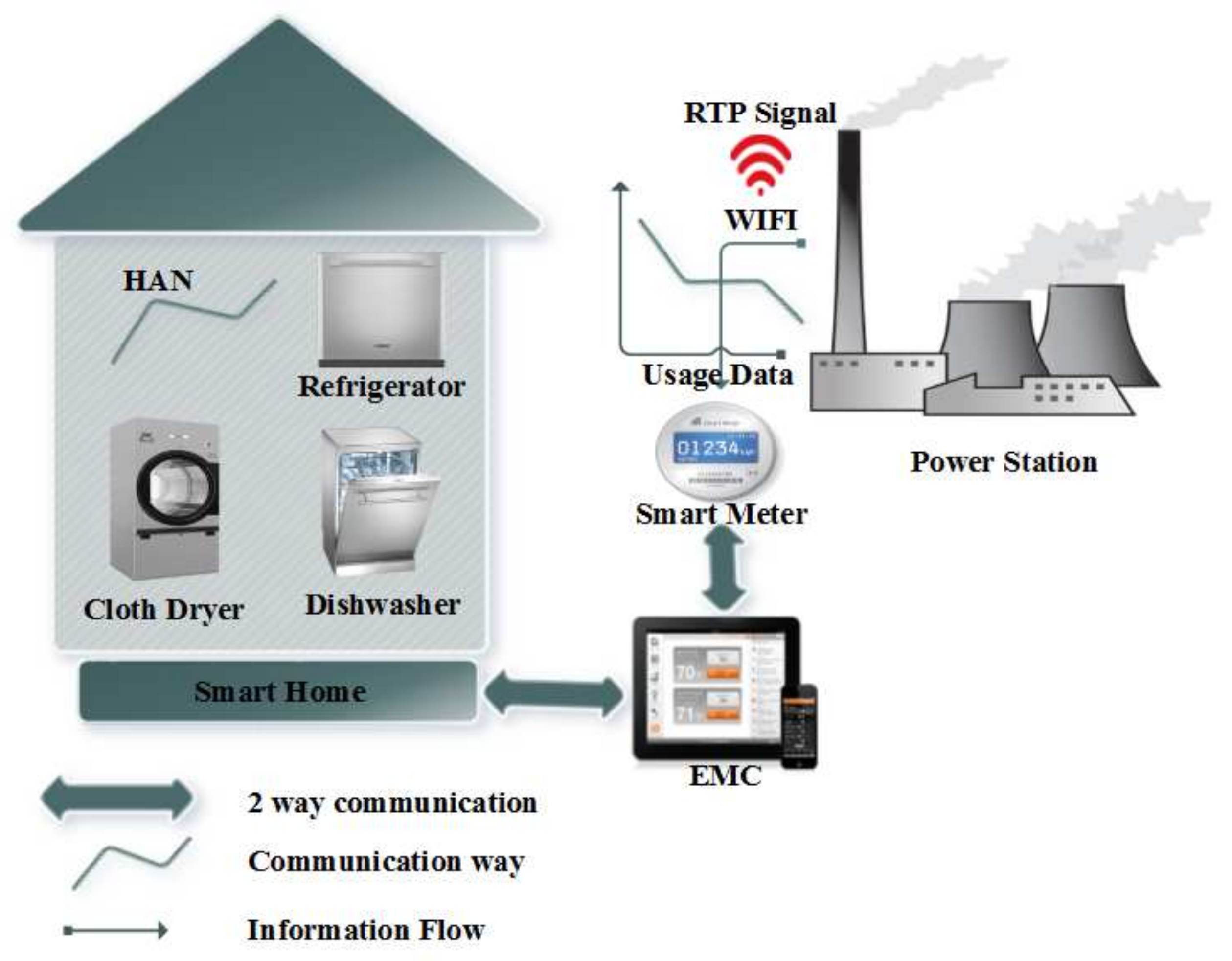
In smart grid, cost minimization, user comfort maximization and PAR reduction are the main objectives to achieve regardless of the energy consumption pattern. In smart home (SH), appliances are scheduled to achieve the minimum cost schedule of each appliance. In SH, there are different smart appliances like advanced metering infrastructure, smart meter (SH), home area network (HAN), smart appliances (SA), energy consumption pattern (ECA), RTP signals and energy management controller (EMC) which controls the on/off status of each appliance and ensure the decision taken for energy consumption. The central scheduler executes the job for appliances and makes the decision whether appliances should be on or off at that particular time slot. We assume there is a system model with multiple homes where each user has different life style, i.e., they use appliances with different power ratings and length of operation time. The conceptual diagram of the smart home is demonstrated in Figure 2.
3.1. HAN
HAN is a network deployed within the home that connects person smart devices, such as computers, telephones, video games, SM, back-haul communication network, data centers, home security system and all those appliances that require Wifi. HAN supports wired and wireless technology like Zigbee, Wifi, WiMax, etc. Typically, HAN comprises of a broadband Internet connection that connects multiple devices via a third party wired or wireless modem. SM is located between HAN and main grid which forwards the accumulated load demand to the main grid via an Internet. The main grid provides pricing signal (i.e., ToU, RTP) based on load demand which later on used for load scheduling.
3.2. AMI
AMI is an assimilation of numerous technologies such as HAN, distributed computing, smart metering and sensors which makes it more digital and informative for both user and system operator. The system incorporating these technologies leads to a smart decision making and user-friendly system.
3.3. EMC
EMC used to monitor the appliances and their energy consumption rating. It contains all the information about appliances, power rating, priorities, threshold, and length of operation and based upon these parameters and the inducted algorithm HEMC take a decision and provide low-cost schedule pattern for the appliances. In this paper, OSR and FA are considered as an optimization algorithm.
3.4. SA
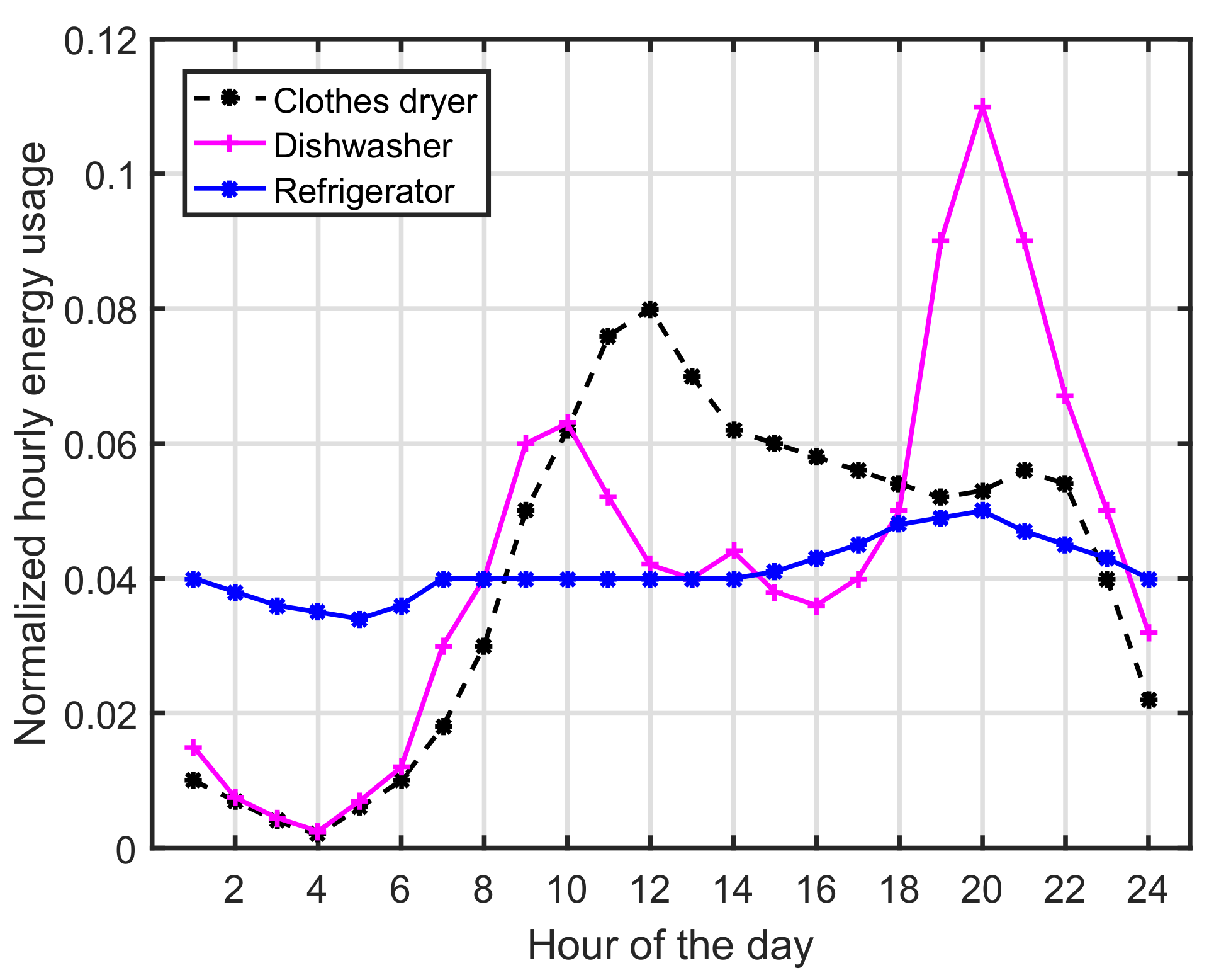
We divide a day into time slots, denoted as T and consider that there is a set of different appliances, denoted as {A1, A2, A3, …, An}. Each appliance has its own energy profile. Energy profile of each appliance is shown in a Figure 3. Each time slot is considered is set as 1 h which is denoted by the parameter . In this paper, we are concerned with shift-able appliances. We assume electricity price of every hour is different and it remains the same throughout the specific time slot. We assume that appliances are categorized into three main categories. Non-shiftable appliances, shiftable and non-interruptible appliances. In this paper, we are primarily concerned with Shiftable appliances. Let assume we have three main appliances cloth dryer, dishwasher, and refrigerator.
The appliances which take more time to accomplish their task can take more than one-time slot. The dishwasher completes its task in three stages such as main wash, final rinse, and heated dry. The cloth dryer has less than an hour duty cycle. It accomplishes its task in only one cycle. The refrigerator has two main stages ice-making and defrost, and only defrost stage of the refrigerator can be scheduled for electricity cost reduction.
3.5. PLC
PLC helps to implement the optimization algorithm provided for it and it provides the visualization through the graphical interface between appliances, SM, and the EMC.
3.6. RTP
Electricity cost is calculated according to the price signal provided by the regulatory authority. For this purpose, different pricing signals can be used which include TOU, IBR, CPP, DAP, RTP, etc. TOU or DAP is predictable and known before the scheduling period, however, RTP changes every next hour. This is the reason scheduling based on RTP is more realistic and gives accurate results for load shifting to off-peak hours from on-peak hours. RTP is considered as more realistic as it is updating the prices of every next hour. In RTP, prices of every next hour vary while it remains the same throughout the specific time slot.
3.7. ECP
ECP of appliances is the essential part of load scheduling mechanism as it provides detail information on energy usage of all appliances. There are three shift-able appliances, cloth dryer, dishwasher, and refrigerator. Figure 3 demonstrates energy profile of appliances for 24 h. We assume that the RTP price is fixed in a month, however, changes constantly for the remaining months. The appliance time slot is fixed as 1 h and the electricity price is assumed to be fixed in that particular time slot to remain same during the one-time slot and the appliances duty cycles are less than . The energy profile shows that 18–24, 8–18 and 2–8 h are on-peak, shoulder peak and off-peak hours, respectively.
4. Problem Formulation
The scheduling problem for an appliance is formulated as an optimization problem using chance constrained optimization (CCO) problem. The problem formulation of three appliances in terms of electricity cost, PAR and waiting time is discussed below. The objective function of the proposed solution is where stands for electricity cost:
4.1. Cost
The cost is calculated from the given equation where is power and is electricity price:
4.2. Load
Load can be computed by the equation below where stands for load and indicates the on off status of appliances:
4.3. PAR
PAR highlights the load peaks and helps to balance the load. It can be formulated by equation below:
4.4. Threshold
P is the electricity price uniformly distributed over [, ] where is the lower limit and is the maximum limit. The appliances are turned on once their electricity price is lesser than the threshold. This equation is taken from [15].
4.5. Waiting Time
Delay or the appliance waiting time is considered to be the appliance average waiting time. It can be computed by given equation where t’s starting time of appliance and ’tr’ is requested time:
4.6. CCO Problem
In this subsection, we seek to determine the feasibility of the proposed solution. To do so, we formulate a CCO problem to map with the home scheduling problem. It defines upper and lower bound limits for power as a power constraint and appliance capacity cannot exceed the maximum load limit of an appliance.
where and are the minimum and maximum power, respectively.
where is less than maximum power limit .
5. Proposed Solution
5.1. Hybrid Schemes
Mathematics programming techniques, including optimal stopping rule and stochastic metaheuristic approaches, are two different streams for combination purpose. Previously, numerous researchers are conducted and it has been noticed that there is a huge potential in building hybrids of mathematical programming such LP, MILP and OSR to the metaheuristic techniques. In fact, different problems can be solved practically in a much better way by exploiting little modification in already existing algorithms. The vital issue is how to combine both techniques in order to achieve maximum benefits. Many hybrid schemes are proposed in past few years. In this paper, we propose different hybrid techniques of OST-GA, OSR-TLBO and OSR-FA. In this concern, there are two basic categories: Collaborative combination, in which both algorithms exchange information, but they are not part of each other. These algorithms work sequentially or parallel. In integrative, one technique is embedded component of another technique. In this paper, we will propose an integrative combination.
5.1.1. Hybrid OSR-GA
We proposed a hybrid technique by combining the OSR and GA. The main aspects of designing a hybrid technique are exploration and exploitation. There must be a balance between local search and global search. We propose a hybrid technique by combining OSR and GA. In case of GA, it has a good convergence rate and performs better in exploration mode while OSR performs better in exploitation mode. In OSR, based on the known information, a decision is taken on when to take the action in order to minimize the cost or maximize the reward. Initially, the hybrid technique works same like the genetic algorithm. At Initial stages, GA steps are followed, such as population generation; we generate a random population of chromosomes. Each of the chromosomes is the candidate solution to the problem. In our case, each bit of chromosomes shows the on/off status of appliances. A fitness function based on the objective function is taken from OSR. For an random appliance, we consider two cost: the electricity cost and the waiting time cost. Our objective is to achieve the minimum cost of the home appliances. This minimization problem can be formulated by optimal stopping rule. The best fitted solution is chosen and recorded as best fit value. Based on the current best solution, a new stream of a population is generated based on crossover and mutation. In GA, the two main genetic control parameters are crossover and mutation. In the crossover, a pair of the parent is selected for each new solution to be produced. In mutation, a single bit of chromosome is replaced which is used to maintain genetic diversity from one generation of a population to the next. These processes ultimately result in the next generation population of chromosomes that is different from the initial generation. It encourages population diversity and helps to prevent premature convergence. The parameters’ list for GA is given in Table 2. Steps of the OSR-GA are mentioned in the Algorithm 1.
| Algorithm 1: OSR-GA Algorithm. |
| Initialize all parameters (population size, number of appliances, selection method, time slots, crossover rate , mutation rate , termination criteria );  |
5.1.2. Hybrid OSR-TLBO
We proposed a hybrid technique by combining the OSR and TLBO. In case of TLBO, it performs better in exploitation mode. TLBO finds the best solution into local search space, while OSR performs better in decision making on random variables in order to minimize expected cost or to expected reward. The best part of TLBO is that among all optimization algorithms it does not rely on any algorithm-specific parameters. So by combining these two algorithms, we can find the optimal solution. Initially, the hybrid technique work like TLBO, such as population generation, learner phase, and teacher phase is same as TLBO. After updating population from teaching and learning phase, fitness function of OSR is applied. This process continues until we find the optimal solution. The proposed technique has better convergence rate and less execution time. List of parameters for TLBO is given in Table 3. Algorithm 2 describes the steps of hybrid OSR-TLBO.
| Algorithm 2: OSR-FA. |
| Initialize system parameters (nPop, MaxIt, T); Initialize algorithm parameters (, , D, I); For all appliances D APP do;  |
5.1.3. Hybrid OSR-FA
We proposed a hybrid technique by combing OSR and FA. FA is inspired by the behavior of fireflies. In FA, the two fundamental functions are to attract matting partner and to attract potential prey. After determining the light intensity and calculating the attractiveness of fireflies the best solution is to find out the fitness of all fireflies from the objective function taken from OSR. This process continues till we find the optimal solution. OSR is a threshold-based policy which depends on the priority of appliances and the threshold. We use simulations to show the properties of OSR. We assume the electricity price is uniformly distributed between [0.01, 0.02] $/KWH. Then the threshold is given by Equation (5). It is observed that intuitively if an appliance is less sensitive to the waiting time, it will wait for the time slot with lower electricity price. Set of parameters for FA are listed in Table 4. The working of hybrid OSR-FA is explained in the Algorithm 3.
| Algorithm 3: OSR-TLBO. |
| Initialize population size, number of subjects, termination criteria; Calculate fitness as objective function;  |
6. Simulation Results
We design the system for a residential area, where we consider 1, 20, 50, 100 and 200 homes with different living style (i.e., set of three appliances with different length of operation time and power ratings). Furthermore, the three main shiftable appliances are cloth dryer, dishwasher and refrigerator. The initial parameters are given in Table 5 and the energy consumption profile is shown in Figure 3. All these appliances are plotted on two different priorities. The priority is consumer defined variable and has a direct impact on the cost and waiting time. The higher priority depicts that the consumer is ready to compromise on cost and lower priority shows that consumer can wait for certain timeslots when the electricity price is low. To avoid randomness in simulation results, we have taken 10 iterations of the whole population and considered the mean of population generation.
In this section, we present the simulation results and analyze the performance of our proposed hybrid algorithms OSR-GA, OSR-TLBO and OSR-FA in RTP environment. We assume the duty cycle of the appliances is 1 h. RTP signal is uniformly distributed between [0.01, 0.02] $/KWH. We assume the RTP remains constant during a month and change with fixed constant for the other months. The detailed comparison is given below.
6.1. Cloth dryer Hybrid OSR-GA
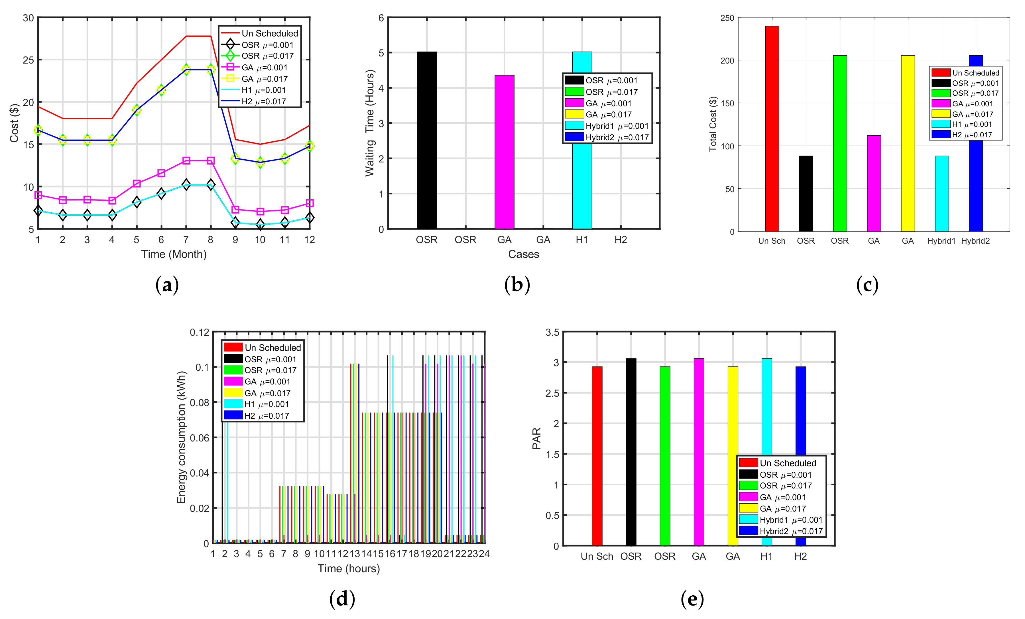
The starting operation of cloth dryer is mostly after breakfast and dinner, which coincides the on-peak hours as shown in Figure 3. Cloth dryer has only one main cycle. Let, represents the power rating of cloth dryer and equation below shows the total energy consumption of cloth dryer and it is shown in Figure 4d.
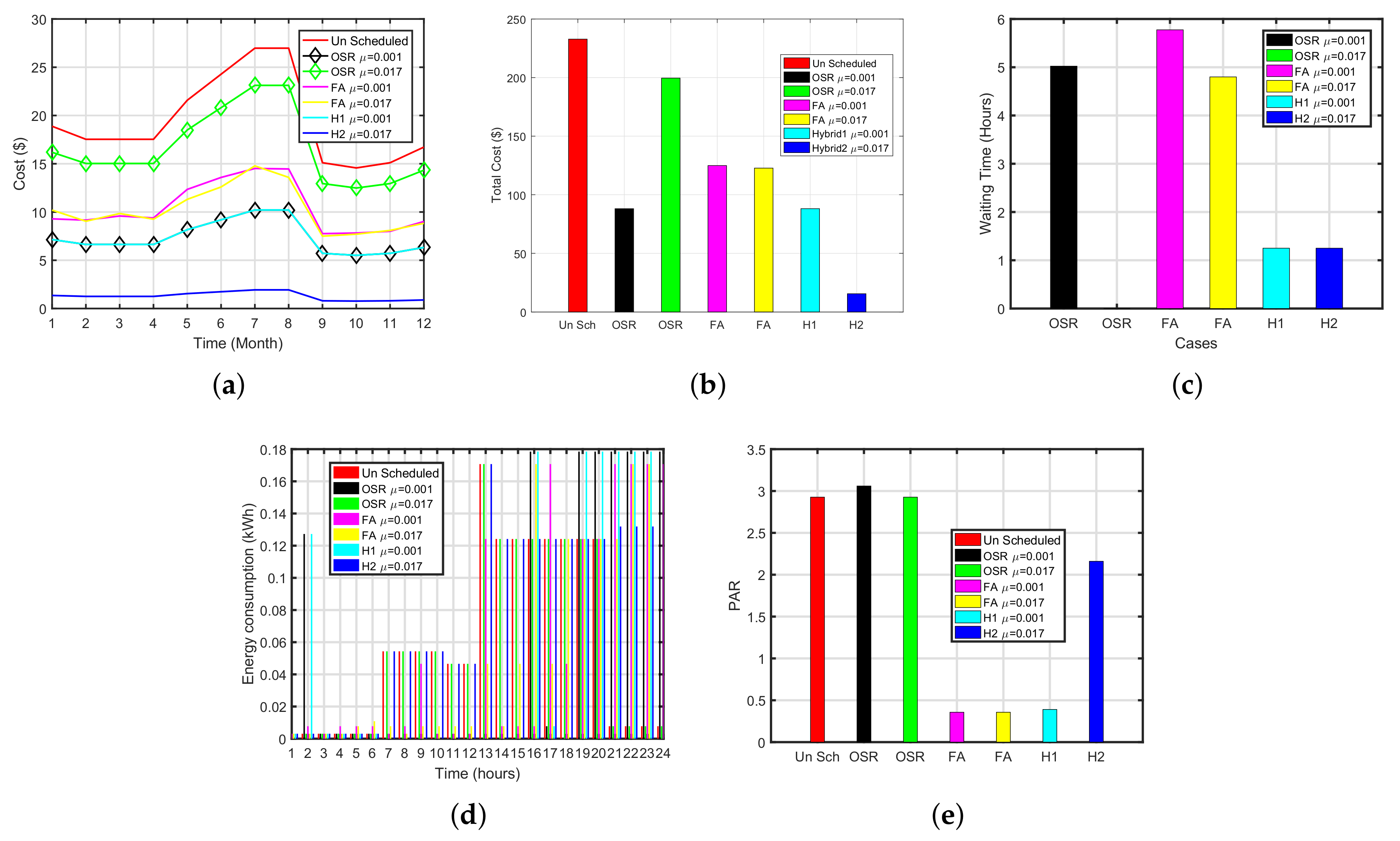
Figure 4a,c show the performance of cloth dryer in terms of cost and waiting time. The simulations for cloth dryer (OSR-GA) are summed up in Table 6. The unscheduled cost acquired by cloth dryer is $232.79. When the priority is set to be low i.e., 0.001 OSR, GA and OSR-GA have reduced the cost by 70%, 60% and 70%, respectively with an average delay of 6.5706, 7.5156 and 6.5 h, respectively. Similarly, when the priority of the cloth dryer is high, i.e., 0.12, OSR, GA and OSR-GA have reduced the cost by 35%, 34% and 35%, respectively. The average delay incurred for priority 0.12 is 3.5833, 3.0455 and 5.0223 h, respectively. OSR-GA performed well as compare to other techniques in terms of waiting time and cost. On the other side, PAR of OSR-GA is optimum in comparison with other algorithms. In Figure 4a, we can clearly observe the significant increase in electricity price for the months 5–9 which interprets that consumers have to pay more for the aforesaid months.
Figure 5a,b show the performance of dishwasher (OSR-GA) in terms of cost and waiting time. The simulations for the dishwasher (OSR-GA) are summed up in Table 7. The unscheduled cost acquired by the dishwasher is $232.79. When the priority is low i.e., 0.001 OSR, GA and OSR-GA have reduced the cost by 62%, 54% and 63%, respectively with an average delay of 5.0223, 4.6429 and 5.0223 h, respectively. Similarly, when the priority of the dishwasher is high i.e., 0.017, OSR, GA and OSR-GA have reduced the cost by 14%, 41% and 14%, respectively. The average delay incurred for priority 0.017 is 0.5, 1.2 and 0.22 h, respectively. OSR-GA performed well as compare to other techniques in terms of waiting time and cost. On the other side, PAR of OSR-GA is optimum in comparison with other algorithms. In Figure 5a, we can clearly observe the significant increase in electricity price for the months 5–9 which interprets that consumers have to pay more for the aforesaid months.
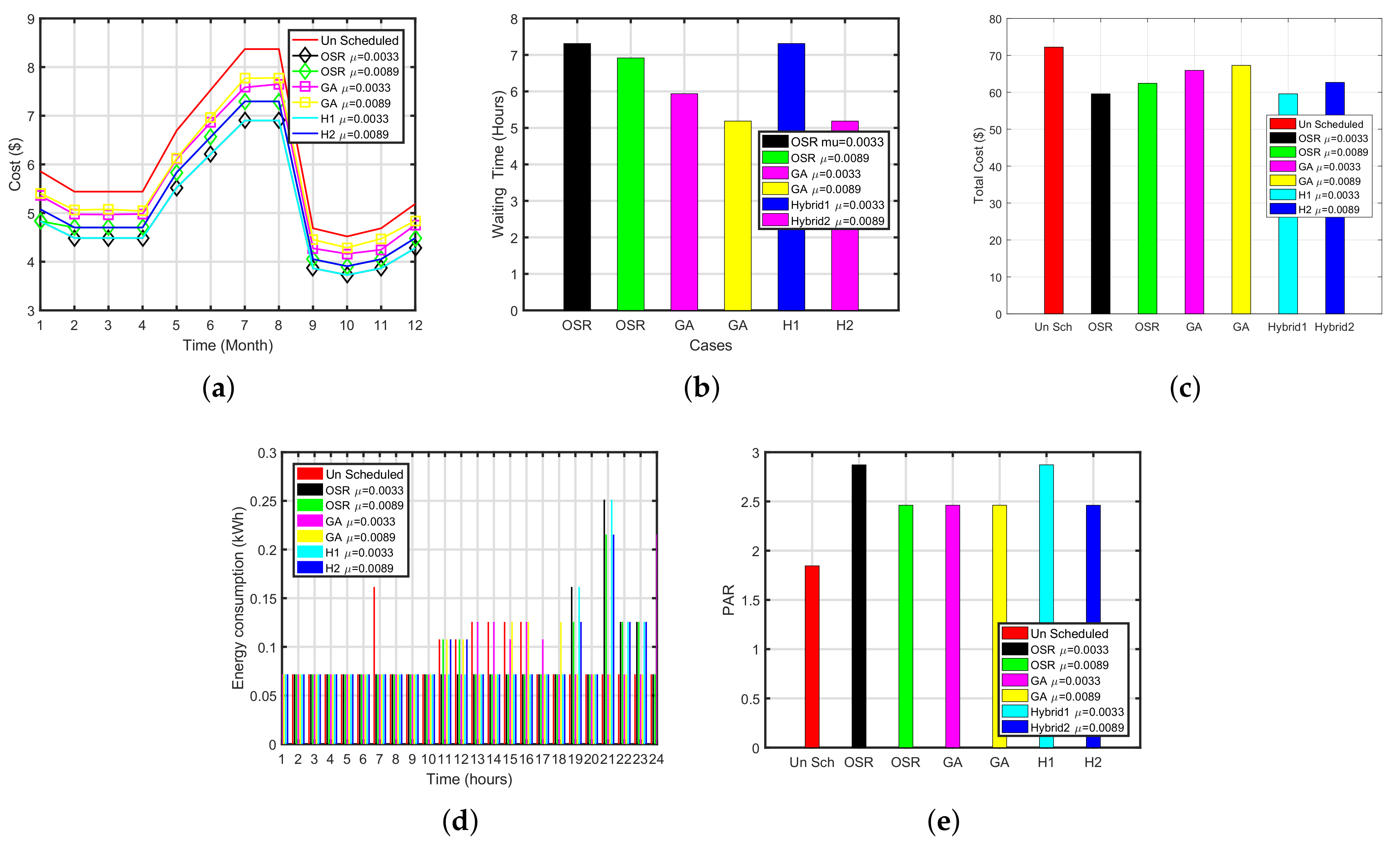
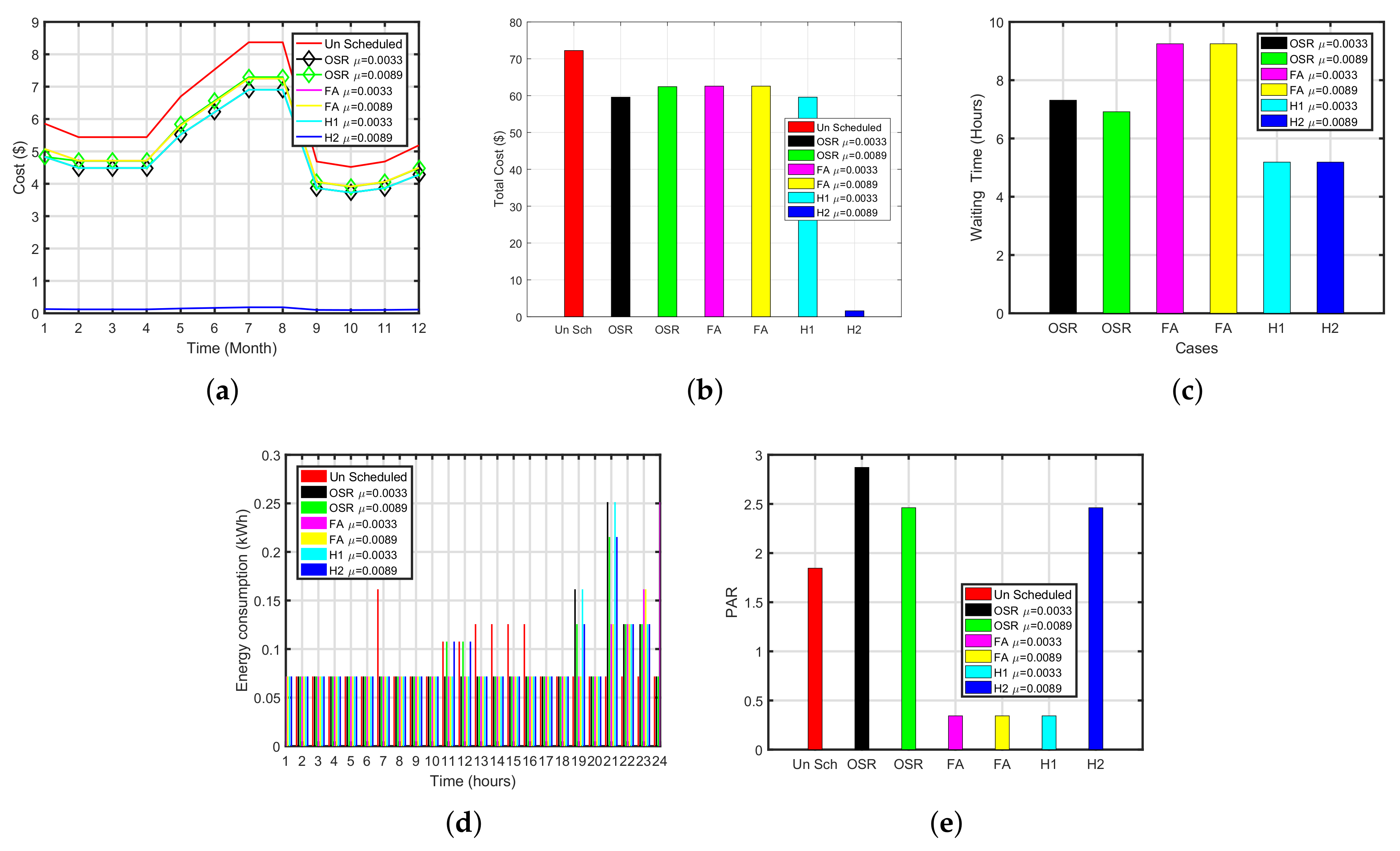
Figure 6a,b show the performance of refrigerator (OSR-GA) in terms of cost and waiting time. The simulations for refrigerator (OSR-GA) are summed up in Table 8. The unscheduled cost acquired by the refrigerator is $72.2305. When the priority is low i.e., 0.0033 OSR, GA and OSR-GA have reduced the cost by 17%, 8% and 17%, respectively with an average delay of 7.3125, 11.7500 and 7.3125 h, respectively. Similarly, when the priority of the refrigerator is high i.e., 0.017, OSR, GA and OSR-GA have reduced the cost by 13%, 4% and 13%, respectively. The average delay incurred for priority 0.0088 is 6.9, 5.5 and 5.1 h, respectively. OSR-GA performed well as compare to other techniques in terms of waiting time and cost. On the other side, PAR of OSR-GA is optimum in comparison with other algorithms. In Figure 6a we can clearly observe the significant increase in electricity price for the months 4–10 which interprets that consumers have to pay more for the aforesaid months.
The simulation results of multiple homes (considering 20, 50, 100 and 200) for cloth dryer are summed up in Table 9 in terms of cost, waiting time and energy consumption.
6.2. Dishwasher
The dishwasher is as flexible as cloth dryer and mostly after breakfast and dinner, It shows spikes, coinciding with the on-peak hours which can be shown in Figure 3. A dishwasher has three stages; main wash, final rinse and heated dry. The dishwasher total energy consumption is represented by the following equation.
One day electricity cost for dish washer is calculated by:
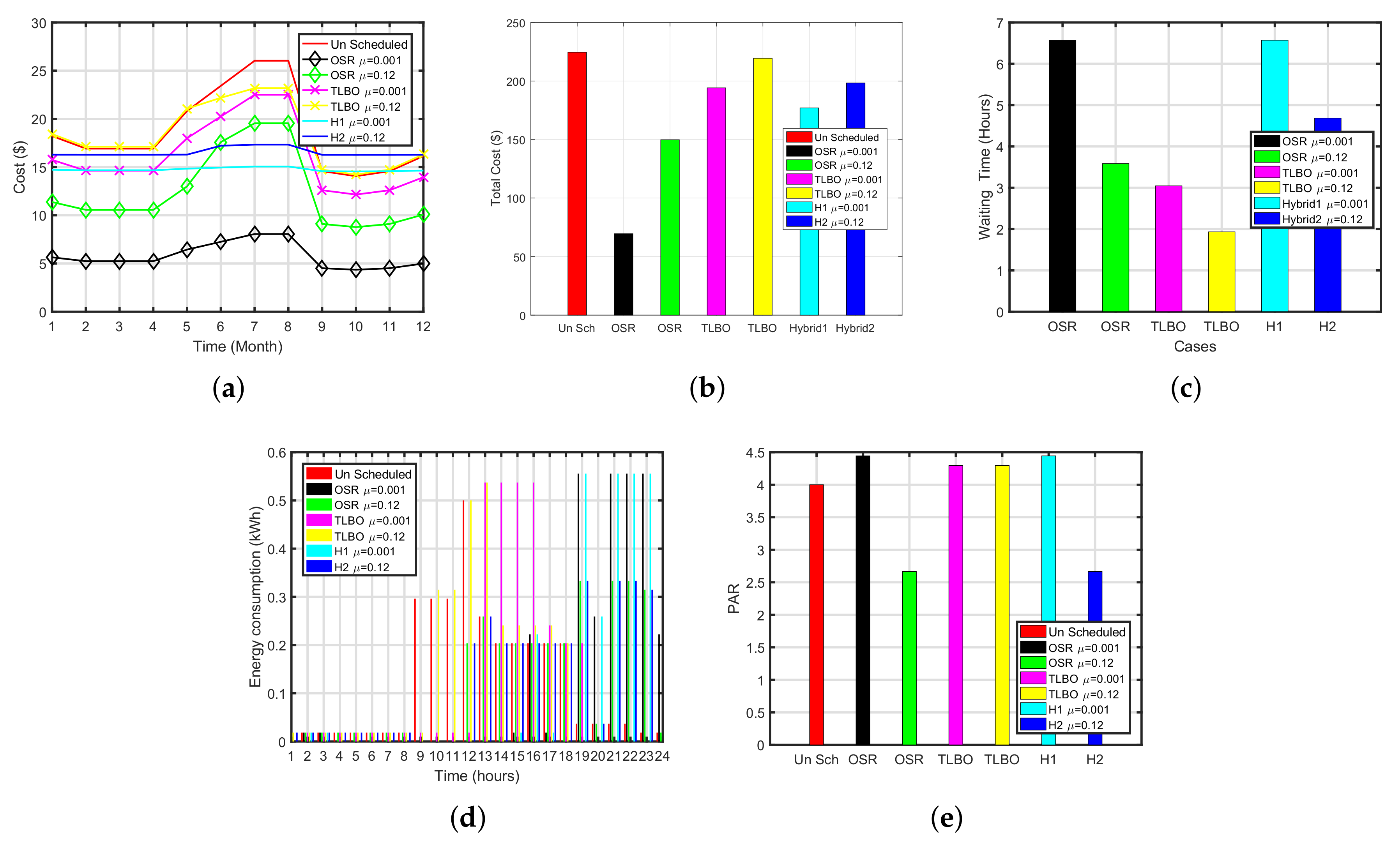
Figure 7a,c illustrate the monthly cost and average waiting time for each month. The result of the simulation is summarized in Table 6. The yearly unscheduled load cost of the cloth dryer (OSR-TLBO) is $232.79. The yearly unscheduled load cost of the cloth dryer is $224.6. When priority is low 0.001 OSR, TLBO and OSR-TLBO have reduced the cost by 70%, 16% and 21% having an average daily delay of 6.5, 3.0 and 6.5 h, respectively. Similarly, when priority is high i.e., 0.12 OSR, TLBO and OSR-TLBO have reduced the cost by 35%, 3.35% and 11% having an average daily delay of 3.5, 12.4, and 2.6 h, respectively.
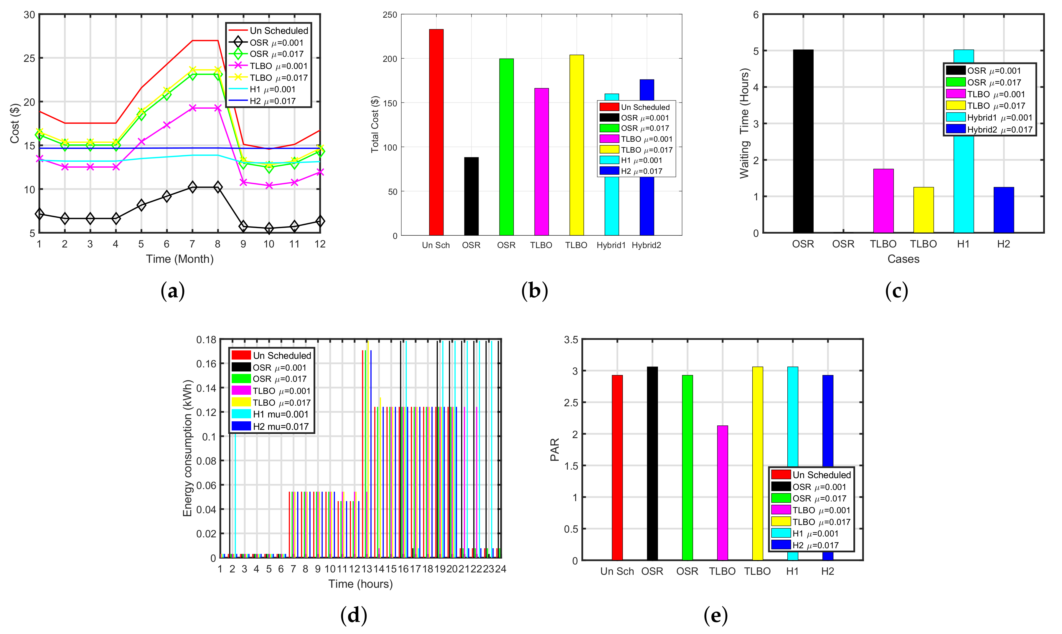
Figure 8a,c illustrate the monthly cost and average waiting time for each month. The result of the simulation is summarized in Table 7. The yearly unscheduled load cost of the dishwasher (OSR-TLBO) is $232.79. The yearly unscheduled load cost of the dishwasher is $232.7986. When priority is low 0.001 OSR, TLBO and OSR-TLBO have reduced the cost by 62%, 92% and 31% having an average daily delay of 5.0223, 1.7500 and 5.0223 h, respectively. Similarly, when priority is high i.e., 0.017 OSR, TLBO and OSR-TLBO have reduced the cost by 14%, 28% and 31% having an average daily delay of 0.5555, 1.2188, and 1.2500 h, respectively.
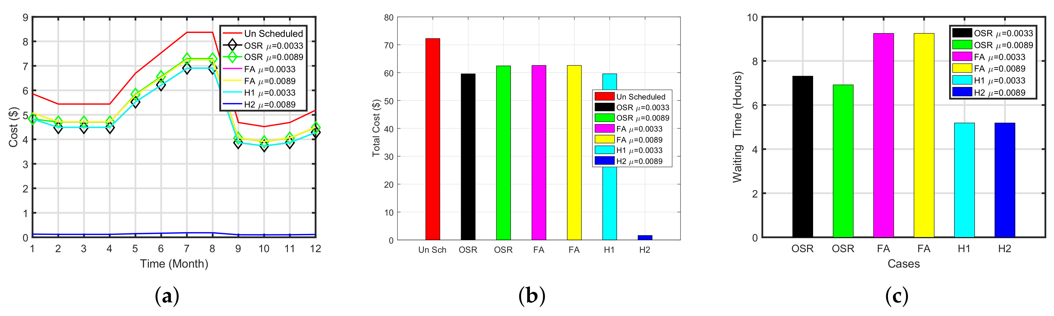
Figure 9a,b illustrate the monthly cost and average waiting time for each month. The result of the simulation is summarized in Table 8. The yearly unscheduled load cost of the refrigerator (OSR-TLBO) is $72.2305. The yearly unscheduled load cost of the refrigerator is $72.2305. When priority is low 0.0033 OSR, TLBO and OSR-TLBO have reduced the cost by 17%, 11% and 24% having an average daily delay of 7.3125, 4.5000 and 7.3125 h, respectively. Similarly, when priority is high i.e., 0.0088 OSR, TLBO and OSR-TLBO have reduced the cost by 13%, 1% and 19% having an average daily delay of 6.916, 1 and 5.1875 h, respectively.
The simulation results of multiple homes (considering 20, 50, 100 and 200) for dishwasher are summed up in Table 10 in terms of cost, waiting time and energy consumption.
6.3. Refrigerator
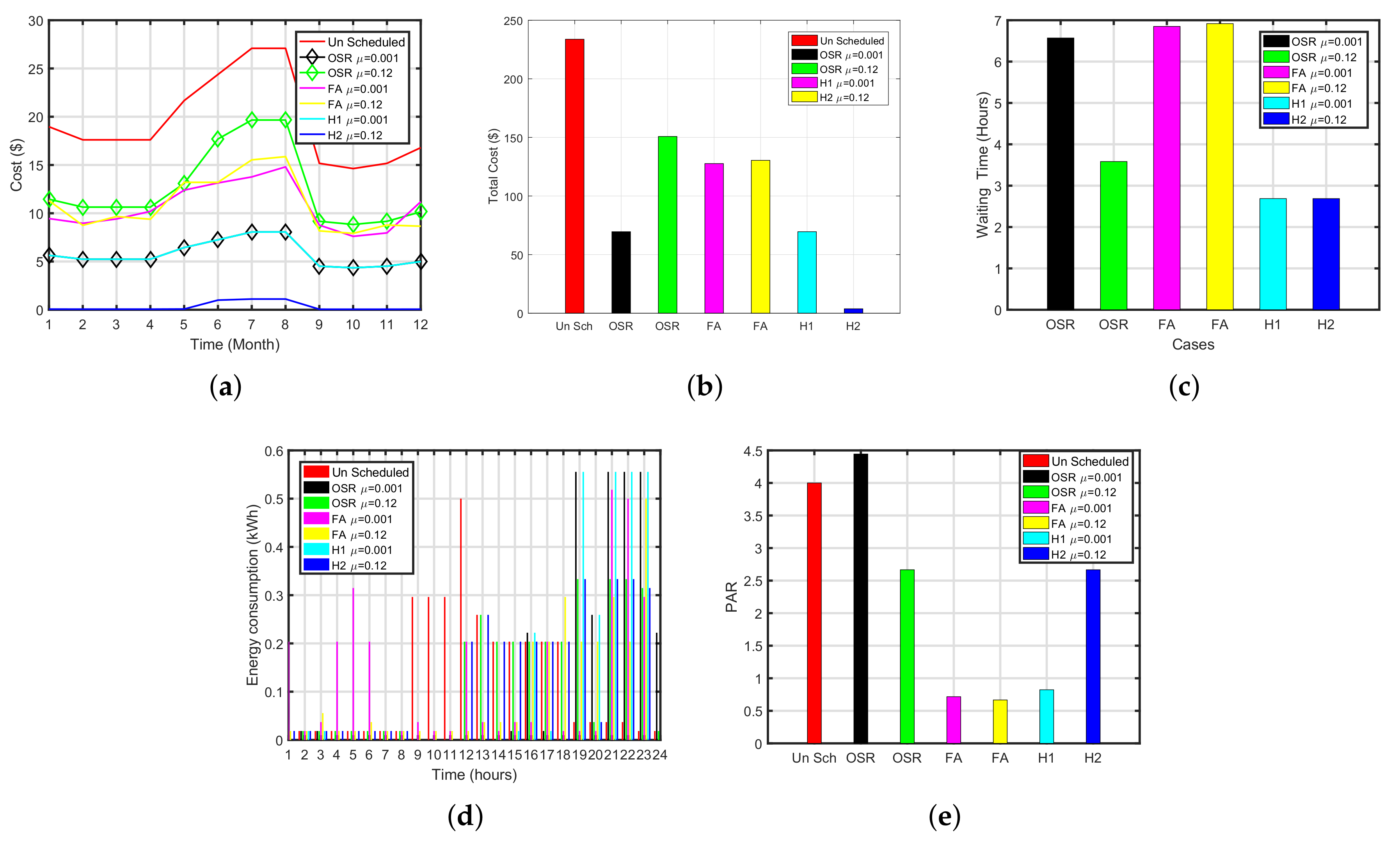
The refrigerator is operated 24 h in a day. There are two states of refrigerator: Icing state and defrost state. We schedule the defrost stage of the refrigerator. In order to obtain the required objectives, we use four techniques to see the effects on average waiting time and cost. The execution cost and waiting time of cloth dryer (OSR-FA) are shown in Figure 10a,c. The summary of the cloth dryer is summed up in Table 8. Simulation results demonstrated that, When the priority of the cloth dryer is low 0.01 OSR, FA and OSR-FA have reduced the cost by 70%, 46% and 70%, respectively with an average delay of 6.5, 7.3 and 2.6 h, respectively. Similarly, when we set the priority of the cloth dryer is set to the higher value 0.12, all schemes have reduced cost by 35%, 44% and 98% with a delay of 3, 5.2, and 2.58 h, respectively. OSR and GA performed better than OSR-FA in terms of cost and waiting time. It is noticed that FA has maximum PAR reduction among others.
The execution cost and waiting time of dishwasher (OSR-FA) are illustrated in Figure 11a,c. The summary of the dishwasher is summed up in Table 8. Simulation results demonstrated that, When the priority of the dishwasher is low 0.01 OSR, FA and OSR-FA have reduced the cost by 62%, 47% and 92%, respectively with an average delay of 5.0, 4.7 and 1.25 h, respectively. Similarly, when we set the priority of the dishwasher is set to the higher value 0.017, all schemes have reduced cost by 14%, 46% and 62% with a delay of 30.5, 4.5, and 0.5 h, respectively.
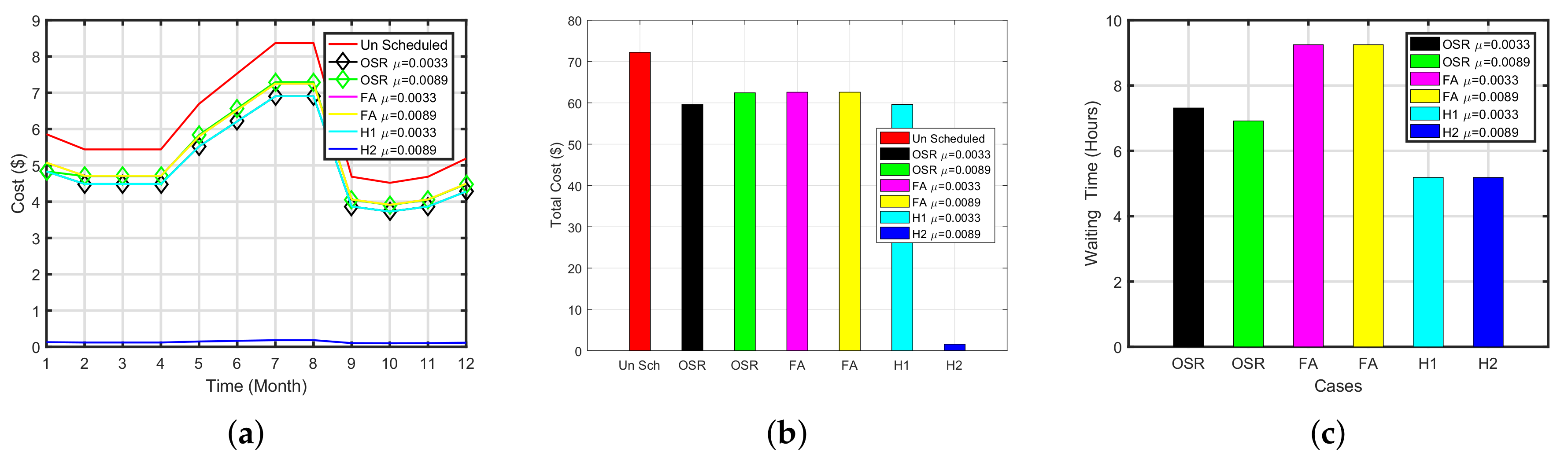
The execution cost and waiting time of refrigerator are illustrated in Figure 12a,c. The summary of the refrigerator is summed up in Table 8. Simulation results demonstrated that, When the priority of the refrigerator is low 0.0033 TLBO, GA, FA and OSR-FA have reduced the cost by 17%, 13% and 92%, respectively with the average delay of 7.3125, 9.2500 and 5.18 h, respectively. Similarly, when we set the priority of the refrigerator to 0.0089, all schemes have reduced cost by 13%, 11% and 17% with a delay of 6.9, 8.9500 and 4.2 h, respectively. OSR-FA and GA performed better than FA in terms of cost and waiting time. It is noticed that FA has maximum PAR reduction among others. It is observed that cost reduction in the refrigerator is significantly less as compared to cloth dryer and dishwasher reduction in cost the defrost state of refrigerator is only considered in the scheduling.
The simulation results of multiple homes (considering 20, 50, 100 and 200) for refrigerator are summed up in Table 11 in terms of cost, waiting time and energy consumption.
7. Feasible Region
A feasible region is the search area which contains all the possible solutions that satisfy the problem constraints. In the current scenario, the objective function relies on the two important factors where cost is the independent factor and electricity consumption is the dependent factor. Both these factors depend upon the electricity price provided by the utility of every particular hour and the corresponding load consumed by the appliances. Figure 13 shows that load can be reduced directly by shifting the load to off-peak hours from on-peak hours.
The highlighted region shows the area which satisfies our objective function. Pictorial representation of possible solution points is represented in Figure 13a. The points P1 (0.0195, 0.00142), P2 (0.0195, 0.0035), P5 (0.075, 0.0103), P6 (0.5, 0.0103) and P4 (0.5, 0.0041) shows the minimum energy consumption and cost. The point P1 shows the minimum possible load coincides the minimum cost. The point P2 shows the maximum electricity cost at the minimum load of appliances. If all appliances are turned On in any specific time slot of max-min prices, resulting in P3 (0.5, 0.0680). Moreover, the points P6 (0.5, 0.0103) and P4 (0.5, 0.0041) represents the bounding limits at maximum load with a min-max price. The connecting line P5 shows that consumer can reduce their load by shifting the load to off-peak hours to on-peak hours. The point P3 is not considered in the feasible region as it crosses the threshold constraint. The following are the possible cases of electricity cost are:
- Min load and Min price
- Min load and Max price
- Max load and Min price
- Max load and Max price
Moreover, the optimum schedule cost should remain less than the unscheduled cost. Now we calculate the FR for cost and waiting time relationship of cloth dryer, which is depicted in Figure 14a. The point P1 shows that when there is no delay in case of unscheduled load scenario the optimum cost is $240.00. The point (P1, P2, P5, and P4) is the feasible region and beyond this limit will create high PAR value.
The FR of the dishwasher is shown in Figure 13b which shows the hourly relationship between cost and energy consumption. Moreover, optimum cost per hour of an unscheduled load is $0.0122. The surrounded region (P1, P2, P4, P5, P6) is the feasible region which illustrates the solution lies within the range of highlighted area and beyond this region, it creates the high peak which is not suitable for consumers and the utility.
FR of dishwasher depicting cost and waiting time relationship is given in Figure 14b. The point P1 shows that when there is no delay in the case of unscheduled scenario the optimum cost is $198.00. It has been observed that the optimum delay occurs at 4.79 h. PAR will be created beyond this limit.
The FR of a refrigerator showing cost and energy consumption relationship is shown in Figure 13c. The optimum cost per hour of the unscheduled load is $0.0217.
8. Conclusions and Future Work
In this paper, the impact of tuning the aforesaid techniques parameters is analyzed in the perspective of cost and waiting time. We have taken three numerous kinds of smart home appliances having different priorities. Additionally, the duty cycle is assumed to solve the problem of cost minimization while considering the waiting time. Price threshold policy and priority of appliances are incorporated to precisely explain the performance parameters of proposed algorithms. OSR-GA, OSR-TLBO, and OSR-FA are the proposed techniques which are compared on the basis of waiting time and cost. The simulations are done in Matlab and the resultsverify that proposed algorithms outperform other algorithms when cost and waiting time is considered. We test our proposed scheme on single smart home as well as multiple smart homes (considering 20, 50, 100, 200 smart homes). It is observed that there exists a trade-off among the performance parameters based on optimization algorithms. The simulation shows that our proposed scheme facilitates the residential customer to participate in DR program.
This work can be further expanded by applying the same scenario on multiple homes with the integration of renewable energy resources and decentralized energy sources in the smart grid. Furthermore, it can be applied to different pricing schemes and we can analyze the performance of scheduler on pricing schemes such as TOU, RTP and CPP, etc. Additionally, these hybrid approaches can be further utilized in different scenarios such as different OTIS with the combination of more number of appliances. Ultimately, the purpose of this work is to evaluate the performance of a small prototype which can be further implemented in the real world scenario. This work can be further enhanced by applying the concept of Fog computing or cloud computing in the same scenario which will improve its scalability.
Author Contributions
All authors have equal contribution.
Conflicts of Interest
The authors declare no conflict of interest.
Nomenclature
| Power rating | |
| Electricity cost | |
| Waiting time | |
| Electricity price at time interval t | |
| Appliances power consumption | |
| Power rating of interruptible appliances | |
| T | Time slot |
| Per day total scheduled load | |
| ON/OFF status of appliances | |
| Z | Threshold |
| Minimum price limit | |
| Maximum price limit | |
| Priority | |
| Initialization time of an appliance | |
| Requested timeslot of an appliance | |
| Timeslot | |
| Minimum power | |
| Maximum power | |
| Maximum power limit | |
| Best learner in teaching phase | |
| Mean value | |
| Random number | |
| D | No of appliances |
| Updated value of pop | |
| Old value of pop | |
| I | Light intensity |
| Attraction |
Abbreviations
| SG | Smart grid |
| SM | Smart meter |
| DSM | Demand side management |
| DR | Demand response |
| RTP | Real time pricing |
| PAR | Peak to average ratio |
| TOU | Time-of-use |
| DAP | Day-ahead-pricing |
| CPP | Critical-peak pricing |
| RTP | Real-time pricing |
| EDP | Extreme-day pricing |
| ED-CPP | Extreme-day cpp |
| MILP | Mixed integer linear programming |
| MINLP | Mixed integer non-linear programming |
| NILP | Non-integer linear programming |
| GA | Genetic algorithm |
| OTI | Operational time interval |
| LOT | Length of operational time |
| HEM | Home energy management |
| EMC | Energy management controller |
| HAN | Home area network |
| TLBO | Teaching learning based optimization |
| SFL | Shuffled frog leaping |
| BPSO | Binary particle swarm optimization |
| ACO | Ant colony optimization |
| OSR | Optimal stopping rule |
| FA | Firefly Algorithm |
| CCO | Chance constrained optimization |
| MG | Microgrid |
| AMI | Advance metering infrastructure |
| SA | Smart appliances |
| PLC | Programmable logic controller |
| ECP | Energy consumption pattern |
| FCFS | First come first serve |
| DE | Differential evolution |
| Pc | Crossover rate |
| Pm | Mutation rate |
| Q | Total available power |
| ET | Power consumption |
| TF | Teaching factor |
| DGA | Demand generation agent |
References
- Javaid, N.; Naseem, M.; Rasheed, M.B.; Mahmood, D.; Khan, S.A.; Alrajeh, N.; Iqbal, Z. A new heuristically optimized Home Energy Management controller for smart grid. Sustain. Cities Soc. 2017, 34, 211–227. [Google Scholar] [CrossRef]
- Mohsenian-Rad, A.H.; Leon-Garcia, A. Optimal residential load control with price prediction in real-time electricity pricing environments. IEEE Trans. Smart Grid 2010, 1, 120–133. [Google Scholar] [CrossRef]
- Pedrasa, M.A.A.; Spooner, T.D.; MacGill, I.F. Coordinated scheduling of residential distributed energy resources to optimize smart home energy services. IEEE Trans. Smart Grid 2010, 1, 134–143. [Google Scholar] [CrossRef]
- Chen, C.; Kishore, S.; Snyder, L.V. An innovative RTP-based residential power scheduling scheme for smart grids. In Proceedings of the 2011 IEEE International Conference on Acoustics, Speech and Signal Processing (ICASSP), Prague, Czech Republic, 22–27 May 2011; pp. 5956–5959. [Google Scholar]
- Caron, S.; Kesidis, G. Incentive-based energy consumption scheduling algorithms for the smart grid. In Proceedings of the 2010 First IEEE International Conference on Smart Grid Communications (SmartGridComm), Gaithersburg, MD, USA, 4–6 October 2010; pp. 391–396. [Google Scholar]
- Mohsenian-Rad, A.H.; Wong, V.W.; Jatskevich, J.; Schober, R. Optimal and autonomous incentive-based energy consumption scheduling algorithm for smart grid. In Proceedings of the Innovative Smart Grid Technologies (ISGT), Gaithersburg, MD, USA, 19–21 January 2010; pp. 1–6. [Google Scholar]
- Molderink, A.; Bakker, V.; Bosman, M.G.; Hurink, J.L.; Smit, G.J. Domestic energy management methodology for optimizing efficiency in smart grids. In Proceedings of the 2009 IEEE Bucharest PowerTech, Bucharest, Romania, 28 June–2 July 2009; pp. 1–7. [Google Scholar]
- Sousa, T.; Morais, H.; Vale, Z.; Faria, P.; Soares, J. Intelligent energy resource management considering vehicle-to-grid: A simulated annealing approach. IEEE Trans. Smart Grid 2012, 3, 535–542. [Google Scholar] [CrossRef]
- Canizes, B.; Soares, J.; Morais, H.; Vale, Z. Modified discrete PSO to increase the delivered energy probability in distribution energy systems. In Proceedings of the 2013 IEEE Symposium on Computational Intelligence Applications In Smart Grid (CIASG), Singapore, 16–19 April 2013; pp. 146–153. [Google Scholar]
- Tsui, K.M.; Chan, S.C. Demand response optimization for smart home scheduling under real-time pricing. IEEE Trans. Smart Grid 2012, 3, 1812–1821. [Google Scholar] [CrossRef]
- Pretorius, H.M.; Delport, G.J. Scheduling of cogeneration facilities operating under the real-time pricing agreement. In Proceedings of the IEEE International Symposium on Industrial Electronics (ISIE’98), Pretoria, South Africa, 7–10 July 1998; Volume 2, pp. 390–395. [Google Scholar]
- Derin, O.; Ferrante, A. Scheduling energy consumption with local renewable micro-generation and dynamic electricity prices. In Proceedings of the First Workshop on Green and Smart Embedded System Technology: Infrastructures, Methods, and Tools, Stockholm, Sweden, 12 April 2010. [Google Scholar]
- Derakhshan, G.; Shayanfar, H.A.; Kazemi, A. The optimization of demand response programs in smart grids. Energy Policy 2016, 94, 295–306. [Google Scholar] [CrossRef]
- Yi, P.; Dong, X.; Iwayemi, A.; Zhou, C.; Li, S. Real-time opportunistic scheduling for residential demand response. IEEE Trans. Smart Grid 2013, 4, 227–234. [Google Scholar] [CrossRef]
- Rasheed, M.B.; Javaid, N.; Ahmad, A.; Awais, M.; Khan, Z.A.; Qasim, U.; Alrajeh, N. Priority and delay constrained demand side management in real-time price environment with renewable energy source. Int. J. Energy Res. 2016, 40, 2002–2021. [Google Scholar] [CrossRef]
- Rahim, S.; Javaid, N.; Ahmad, A.; Khan, S.A.; Khan, Z.A.; Alrajeh, N.; Qasim, U. Exploiting heuristic algorithms to efficiently utilize energy management controllers with renewable energy sources. Energy Build. 2016, 129, 452–470. [Google Scholar] [CrossRef]
- Logenthiran, T.; Srinivasan, D.; Shun, T.Z. Demand side management in smart grid using heuristic optimization. IEEE Trans. Smart Grid 2012, 3, 1244–1252. [Google Scholar] [CrossRef]
- Muralitharan, K.; Sakthivel, R.; Shi, Y. Multiobjective optimization technique for demand side management with load balancing approach in smart grid. Neurocomputing 2016, 177, 110–119. [Google Scholar] [CrossRef]
- Mary, G.A.; Rajarajeswari, R. Smart Grid Cost Optimization Using Genetic Algorithm. Int. J. Res. Eng. Technol. 2014, 3, 282–287. [Google Scholar]
- Zhang, J.; Wu, Y.; Guo, Y.; Wang, B.; Wang, H.; Liu, H. A hybrid harmony search algorithm with differential evolution for day-ahead scheduling problem of a microgrid with consideration of power flow constraints. Appl. Energy 2016, 183, 791–804. [Google Scholar] [CrossRef]
- Reddy, S.S.; Park, J.Y.; Jung, C.M. Optimal operation of microgrid using hybrid differential evolution and harmony search algorithm. Front. Energy 2016, 10, 355–362. [Google Scholar] [CrossRef]
- Khatib, T.; Mohamed, A.; Sopian, K. Optimization of a PV/wind micro-grid for rural housing electrification using a hybrid iterative/genetic algorithm: Case study of Kuala Terengganu, Malaysia. Energy Build. 2012, 47, 321–331. [Google Scholar] [CrossRef]
- Roy, K.; Mandal, K.K. Hybrid optimization algorithm for modeling and management of micro grid connected system. Front. Energy 2014, 8, 305–314. [Google Scholar] [CrossRef]
- Moghaddam, A.A.; Seifi, A.; Niknam, T.; Pahlavani, M.R.A. Multi-objective operation management of a renewable MG (micro-grid) with back-up micro-turbine/fuel cell/battery hybrid power source. Energy 2011, 36, 6490–6507. [Google Scholar] [CrossRef]
- Güçyetmez, M.; Çam, E. A new hybrid algorithm with genetic-teaching learning optimization (G-TLBO) technique for optimizing of power flow in wind-thermal power systems. Electr. Eng. 2016, 98, 145–157. [Google Scholar] [CrossRef]
- Javaid, N.; Ullah, I.; Akbar, M.; Iqbal, Z.; Khan, F.A.; Alrajeh, N.; Alabed, M.S. An intelligent load management system with renewable energy integration for smart homes. IEEE Access 2017, 5, 13587–13600. [Google Scholar] [CrossRef]
- Rasheed, M.B.; Javaid, N.; Awais, M.; Khan, Z.A.; Qasim, U.; Alrajeh, N.; Iqbal, Z.; Javaid, Q. Real time information based energy management using customer preferences and dynamic pricing in smart homes. Energies 2016, 9, 542. [Google Scholar] [CrossRef]
- Ahmad, A.; Khan, A.; Javaid, N.; Hussain, H.M.; Abdul, W.; Almogren, A.; Alamri, A.; Azim Niaz, I. An Optimized Home Energy Management System with Integrated Renewable Energy and Storage Resources. Energies 2017, 10, 549. [Google Scholar] [CrossRef]
- Amini, M.H.; Nabi, B.; Haghifam, M.R. Load management using multi-agent systems in smart distribution network. In Proceedings of the 2013 IEEE Power and Energy Society General Meeting (PES), Vancouver, BC, Canada, 21–25 July 2013; pp. 1–5. [Google Scholar]
- Bahrami, S.; Wong, V.W.; Huang, J. An online learning algorithm for demand response in smart grid. IEEE Trans. Smart Grid 2017, PP, 1. [Google Scholar] [CrossRef]
- Bahrami, S.; Parniani, M.; Vafaeimehr, A. A modified approach for residential load scheduling using smart meters. In Proceedings of the 2012 3rd IEEE PES International Conference and Exhibition on Innovative Smart Grid Technologies (ISGT Europe), Berlin, Germany, 14–17 October 2012; pp. 1–8. [Google Scholar]
- Amini, M.H.; Frye, J.; Ilić, M.D.; Karabasoglu, O. Smart residential energy scheduling utilizing two stage mixed integer linear programming. In Proceedings of the 2015 North American Power Symposium (NAPS), Charlotte, NC, USA, 4–6 October 2015; pp. 1–6. [Google Scholar]
- Mohammadi, A.; Mehrtash, M.; Kargarian, A. Diagonal quadratic approximation for decentralized collaborative TSO+ DSO optimal power flow. IEEE Trans. Smart Grid 2018. [Google Scholar] [CrossRef]
- Bahrami, S.; Amini, M.H.; Shafie-khah, M.; Catalao, J.P. A Decentralized Electricity Market Scheme Enabling Demand Response Deployment. IEEE Power Energy Soc. 2017. [Google Scholar] [CrossRef]
- Yalcin, T.; Ozdemir, M. Pattern recognition method for identifying smart grid power quality disturbance. In Proceedings of the 2016 17th International Conference on Harmonics and Quality of Power (ICHQP), Minas Gerais, Brazil, 16–19 October 2016; pp. 903–907. [Google Scholar]
- Gajowniczek, K.; Ząbkowski, T. Data mining techniques for detecting household characteristics based on smart meter data. Energies 2015, 8, 7407–7427. [Google Scholar] [CrossRef]
- Singh, S.; Yassine, A. Big Data Mining of Energy Time Series for Behavioral Analytics and Energy Consumption Forecasting. Energies 2018, 11, 452. [Google Scholar] [CrossRef]
- Gajowniczek, K.; Ząbkowski, T. Electricity forecasting on the individual household level enhanced based on activity patterns. PLoS ONE 2017, 12, e0174098. [Google Scholar] [CrossRef] [PubMed]
- Pooranian, Z.; Nikmehr, N.; Najafi-Ravadanegh, S.; Mahdin, H.; Abawajy, J. Economical and environmental operation of smart networked microgrids under uncertainties using NSGA-II. In Proceedings of the 2016 24th International Conference on Software, Telecommunications and Computer Networks (SoftCOM), Split, Croatia, 22–24 September 2016; pp. 1–6. [Google Scholar]
- Naranjo, P.G.V.; Pooranian, Z.; Shojafar, M.; Conti, M.; Buyya, R. FOCAN: A Fog-supported Smart City Network Architecture for Management of Applications in the Internet of Everything Environments. arXiv, 2017; arXiv:1710.01801. [Google Scholar]
- De la Torre, S.; Arroyo, J.M.; Conejo, A.J.; Contreras, J. Price maker self-scheduling in a pool-based electricity market: A mixed-integer LP approach. IEEE Trans. Power Syst. 2002, 17, 1037–1042. [Google Scholar] [CrossRef]
Figure 1.
Schematic Manuscript Overview.

Figure 2.
Proposed System Model.

Figure 3.
Energy Profile of Appliances.

Figure 4.
Hybrid Plots for Cloth Dryer (OSR-GA). (a) Monthly Cost of Cloth Dryer (OSR-GA), (b) Total Cost of Cloth Dryer (OSR-GA), (c) Waiting Time of Cloth Dryer (OSR-GA), (d) Energy Consumption of Cloth Dryer (OSR-GA), (e) PAR of Cloth Dryer (OSR-GA).
Figure 4.
Hybrid Plots for Cloth Dryer (OSR-GA). (a) Monthly Cost of Cloth Dryer (OSR-GA), (b) Total Cost of Cloth Dryer (OSR-GA), (c) Waiting Time of Cloth Dryer (OSR-GA), (d) Energy Consumption of Cloth Dryer (OSR-GA), (e) PAR of Cloth Dryer (OSR-GA).

Figure 5.
Hybrid Plots for Dish Washer (OSR-GA). (a) Monthly Cost of Dish Washer (OSR-GA), (b) Waiting Time of Dish Washer (OSR-GA), (c) Total Cost of Dish Washer (OSR-GA), (d) Energy Consumption of Dish Washer (OSR-GA), (e) PAR of Dish Washer (OSR-GA).
Figure 5.
Hybrid Plots for Dish Washer (OSR-GA). (a) Monthly Cost of Dish Washer (OSR-GA), (b) Waiting Time of Dish Washer (OSR-GA), (c) Total Cost of Dish Washer (OSR-GA), (d) Energy Consumption of Dish Washer (OSR-GA), (e) PAR of Dish Washer (OSR-GA).

Figure 6.
Hybrid Plots for Refrigerator (OSR-GA). (a) Monthly Cost of Refrigerator (OSR-GA), (b) Waiting Time of Refrigerator (OSR-GA), (c) Total Cost of Dish Washer (OSR-GA), (d) Energy Consumption of Refrigerator (OSR-GA), (e) PAR of Refrigerator (OSR-GA).
Figure 6.
Hybrid Plots for Refrigerator (OSR-GA). (a) Monthly Cost of Refrigerator (OSR-GA), (b) Waiting Time of Refrigerator (OSR-GA), (c) Total Cost of Dish Washer (OSR-GA), (d) Energy Consumption of Refrigerator (OSR-GA), (e) PAR of Refrigerator (OSR-GA).

Figure 7.
Hybrid Plots for Cloth Dryer (OSR-TLBO). (a) Monthly Cost of Cloth Dryer (OSR-TLBO), (b) Total Cost of Cloth Dryer (OSR-TLBO), (c) Waiting Time of Cloth Dryer (OSR-TLBO), (d) Energy Consumption of Cloth Dryer (OSR-TLBO), (e) PAR of Cloth Dryer (OSR-TLBO).
Figure 7.
Hybrid Plots for Cloth Dryer (OSR-TLBO). (a) Monthly Cost of Cloth Dryer (OSR-TLBO), (b) Total Cost of Cloth Dryer (OSR-TLBO), (c) Waiting Time of Cloth Dryer (OSR-TLBO), (d) Energy Consumption of Cloth Dryer (OSR-TLBO), (e) PAR of Cloth Dryer (OSR-TLBO).

Figure 8.
Hybrid Plots for Dish Washer (OSR-TLBO). (a) Monthly Cost of Dish Washer (OSR-TLBO), (b) Total Cost of Dish Washer (OSR-TLBO), (c) Waiting Time of Dish Washer (OSR-TLBO), (d) Energy Consumption of Dish Washer (OSR-TLBO), (e) PAR of Dish Washer (OSR-TLBO).
Figure 8.
Hybrid Plots for Dish Washer (OSR-TLBO). (a) Monthly Cost of Dish Washer (OSR-TLBO), (b) Total Cost of Dish Washer (OSR-TLBO), (c) Waiting Time of Dish Washer (OSR-TLBO), (d) Energy Consumption of Dish Washer (OSR-TLBO), (e) PAR of Dish Washer (OSR-TLBO).

Figure 9.
Hybrid Plots for Refrigerator (OSR-TLBO). (a) Monthly Cost of Refrigerator (OSR-TLBO), (b) Waiting Time of Refrigerator (OSR-TLBO), (c) Total Cost of Dish Washer (OSR-TLBO), (d) Energy Consumption of Refrigerator (OSR-TLBO), (e) PAR of Refrigerator (OSR-TLBO).
Figure 9.
Hybrid Plots for Refrigerator (OSR-TLBO). (a) Monthly Cost of Refrigerator (OSR-TLBO), (b) Waiting Time of Refrigerator (OSR-TLBO), (c) Total Cost of Dish Washer (OSR-TLBO), (d) Energy Consumption of Refrigerator (OSR-TLBO), (e) PAR of Refrigerator (OSR-TLBO).

Figure 10.
Hybrid Plots for Cloth Dryer (OSR-FA). (a) Monthly Cost of Cloth Dryer (OSR-FA), (b) Total Cost of Cloth Dryer (OSR-FA), (c) Waiting Time of Cloth Dryer (OSR-FA), (d) Energy Consumption of Cloth Dryer (OSR-FA), (e) PAR of Cloth Dryer (OSR-FA).
Figure 10.
Hybrid Plots for Cloth Dryer (OSR-FA). (a) Monthly Cost of Cloth Dryer (OSR-FA), (b) Total Cost of Cloth Dryer (OSR-FA), (c) Waiting Time of Cloth Dryer (OSR-FA), (d) Energy Consumption of Cloth Dryer (OSR-FA), (e) PAR of Cloth Dryer (OSR-FA).

Figure 11.
Hybrid Plots for Dish Washer (OSR-FA). (a) Monthly Cost of Dish Washer (OSR-FA), (b) Total Cost of Dish Washer (OSR-FA), (c) Waiting Time of Dish Washer (OSR-FA), (d) Energy Consumption of Dish Washer (OSR-FA), (e) PAR of Dish Washer (OSR-FA).
Figure 11.
Hybrid Plots for Dish Washer (OSR-FA). (a) Monthly Cost of Dish Washer (OSR-FA), (b) Total Cost of Dish Washer (OSR-FA), (c) Waiting Time of Dish Washer (OSR-FA), (d) Energy Consumption of Dish Washer (OSR-FA), (e) PAR of Dish Washer (OSR-FA).

Figure 12.
Hybrid Plots for Refrigerator (OSR-FA). (a) Monthly Cost of Refrigerator (OSR-FA), (b) Total Cost of Refrigerator (OSR-FA), (c) Waiting Time of Refrigerator (OSR-FA), (d) Energy Consumption of Refrigerator (OSR-FA), (e) PAR of Refrigerator (OSR-FA).
Figure 12.
Hybrid Plots for Refrigerator (OSR-FA). (a) Monthly Cost of Refrigerator (OSR-FA), (b) Total Cost of Refrigerator (OSR-FA), (c) Waiting Time of Refrigerator (OSR-FA), (d) Energy Consumption of Refrigerator (OSR-FA), (e) PAR of Refrigerator (OSR-FA).

Figure 13.
Cont. (a) Energy Consumption and Cost of Cloth Dryer, (b) Energy Consumption and Cost of Dish Washer, (c) Energy Consumption and Cost of Refrigerator.
Figure 13.
Cont. (a) Energy Consumption and Cost of Cloth Dryer, (b) Energy Consumption and Cost of Dish Washer, (c) Energy Consumption and Cost of Refrigerator.

Figure 14.
Cont. (a) Energy Consumption and Cost of Cloth Dryer, (b) Energy Consumption and Cost of Dish Washer, (c) Energy Consumption and Cost of Refrigerator.
Figure 14.
Cont. (a) Energy Consumption and Cost of Cloth Dryer, (b) Energy Consumption and Cost of Dish Washer, (c) Energy Consumption and Cost of Refrigerator.


Table 1.
Summarized Related Work.
| Reference | Technique | Objective | Limitation |
|---|---|---|---|
| Price maker Self-Scheduling in a Pool-Based EM [41] | MILP | Cost minimization | Extensive computation |
| Optimization of DR programs [13] | TLBO and SFL | Cost minimization | Delay, user comfort and PAR are ignored |
| Real-Time opportunistic Scheduling [14] | OSR | Minimize cost and waiting time | PAR neglected |
| Priority and delay constrained DSM [15] | FCFS, MFCFS, PEEDF, and OSR | cost minimization and energy consumption through RESs | Individual appliance scheduling is ignored |
| Energy management controllers with RESs (16) [16] | ACO, BPSO and GA | PAR reduction and cost | User comfort and privacy issues |
| DSM in smart grid [17] | EA | Minimize Cost and PAR | User comfort is ignored |
| Multiobjective optimization technique for DSM [18] | MOEA | Cost and delay | PAR is not considered |
| Smart grid cost optimization using GA [19] | GA | Minimize cost | Consider inelastic load |
| A day-ahead scheduling model for the optimal operation in Microgrid [20] | HSA and DE | Total generation cost and operational cost minimization, introduced power flow constraints, consider transmission line losses | Ignore uncertainty of PV and WT |
| Hybrid deferential evolution with harmony search algorithm [21] | DEHS | Cost minimization, uncertainty of WT and PV is modeled | Pollutant emissions are not considered |
| Optimization of hybrid PV and WT [22] | Hybrid itrative and GA | Minimize system cost, tilt angel optimization Improve inverter efficiency, Optimal size ratio of PV, WT, storage battery and inverter has been achieved | Transmission losses not considered |
| Hybrid artificial bee colony (ABC) approach [23] | Hybrid ABC | Fuel and maintenance cost minimization, selection of best power generator under various load demands | Uncertainty of PV and WT |
| Adaptive modified particle swarm optimization algorithm [24] | AMPSO and Hybrid PSO | Operational cost minimization and reduce pollutant emissions, RESs integration | Increase operational cost |
| Genetic teaching learning-based optimization (G-TLBO) [25] | GA and TLBO | Minimize fuel cost and less execution time, good for large energy structure Great energy saving | Reactive line losses are neglected |
Table 2.
GA parameters and values.
| Parameter | Value |
|---|---|
| Population Size | 50 |
| Selection | Tournament Selection |
| Elite Count | 2 |
| Crossover | 0.9 |
| Mutation | 0.1 |
| Stopping Criteria | Max. Generation |
| Max. Generation | 100 |
Table 3.
TLBO parameters and values.
| Parameter | Value |
|---|---|
| Population Size | 24 |
| App | 3 |
| Hour | 24 |
Table 4.
FA parameters and values.
| Parameter | Value |
|---|---|
| Population Size | 24 |
| App | 3 |
| Max It | 10 |
| Varmin | 10 |
| Varmax | 10 |
| Gamma | 1 |
| Beta | 2 |
| Alpha | 0.2 |
Table 5.
Parameters of Appliances.
| Appliances | Average Power (kW) | LOT (hours) | Priority () |
|---|---|---|---|
| Clothdryer | 3.0 | 0.75 | [0.01, 0.12] |
| Dishwasher | 0.8 | 1.75 | [0.001, 0.017] |
| Refrigerator | 0.089 | 24 | [0.0033, 0.0089] |
Table 6.
Cloth Dryer Simulation Statistics.
| Hybrid | Technique | Priority | Average Cost/Month | Reduction in Cost (%) | Average Delay in Hours/Day |
|---|---|---|---|---|---|
| OSR-GA | OSR | 0.01 | 29.7400 | 70.25 | 6.5706 |
| 0.12 | 64.5000 | 35.50 | 3.5833 | ||
| GA | 0.01 | 40.1200 | 60 | 7.5156 | |
| 0.12 | 65.4600 | 34 | 3.4091 | ||
| OSR-GA | 0.01 | 29.7418 | 70.2582 | 6.5706 | |
| 0.12 | 64.4998 | 35.5002 | 5.0223 | ||
| OSR-TLBO | OSR | 0.01 | 29.7400 | 70.25 | 6.5706 |
| 0.12 | 64.5000 | 35.50 | 3.5833 | ||
| TLBO | 0.01 | 73 | 16 | 3.0 | |
| 0.12 | 83 | 3.35 | 2.4091 | ||
| OSR-TLBO | 0.01 | 58 | 21 | 6.5 | |
| 0.12 | 68 | 11 | 2.6 | ||
| OSR-FA | OSR | 0.01 | 29.7400 | 70.25 | 6.5706 |
| 0.12 | 64.5000 | 35.50 | 3.5833 | ||
| FA | 0.01 | 53.8949 | 46.1050 | 7.3205 | |
| 0.12 | 55.3693 | 44.1913 | 5.2242 | ||
| OSR-FA | 0.01 | 29.7418 | 70.2582 | 2.6875 | |
| 0.12 | 1.6030 | 98.3970 | 2.5875 |
Table 7.
Dishwasher Simulation Statistics.
| Hybrid | Technique | Priority | Average Cost/Month | Reduction in Cost (%) | Average Delay in Hours/Day |
|---|---|---|---|---|---|
| OSR-GA | OSR | 0.001 | 37.8458 | 62.1542 | 5.0223 |
| 0.017 | 85.7143 | 14.2857 | 0.5555 | ||
| GA | 0.001 | 45.2012 | 54 | 4.6429 | |
| 0.017 | 58.1443 | 41 | 1.2188 | ||
| OSR-GA | 0.001 | 36.7558 | 63.2442 | 5.0223 | |
| 0.017 | 85.7143 | 14.2857 | 0.22 | ||
| OSR-TLBO | OSR | 0.001 | 37.8458 | 62.1542 | 5.0223 |
| 0.017 | 85.7143 | 14.2857 | 0.5555 | ||
| TLBO | 0.001 | 27.2866 | 92 | 2.7500 | |
| 0.017 | 71.3850 | 28 | 1.6250 | ||
| OSR-TLBO | 0.001 | 58.7037 | 31.2963 | 5.0223 | |
| 0.017 | 68.0152 | 20.9848 | 1.2500 | ||
| OSR-FA | OSR | 0.001 | 37.8458 | 62.1542 | 5.0223 |
| 0.017 | 85.7143 | 14.2857 | 0.5555 | ||
| FA | 0.001 | 52.9677 | 47.03 | 4.7857 | |
| 0.017 | 53.5672 | 46 | 4.6696 | ||
| OSR-FA | 0.001 | 6.66 | 92 | 1.25 | |
| 0.017 | 37 | 62 | 0.5 |
Table 8.
Refrigerator Simulation Statistics.
| Hybrid | Technique | Priority | Average Cost/Month | Reduction in Cost (%) | Average Delay in Hours/Day |
|---|---|---|---|---|---|
| OSR-GA | OSR | 0.0033 | 82.4841 | 17 | 7.3125 |
| 0.0089 | 86.4284 | 13 | 6.9167 | ||
| GA | 0.0033 | 91.7838 | 8 | 11.7500 | |
| 0.0089 | 95.8347 | 4 | 5.5000 | ||
| OSR-GA | 0.0033 | 82.4841 | 17.5159 | 7.3125 | |
| 0.0089 | 86.7690 | 13.2310 | 5.1875 | ||
| OSR-TLBO | OSR | 0.0033 | 82.4841 | 17 | 7.3125 |
| 0.0089 | 86.4284 | 13 | 6.9167 | ||
| TLBO | 0.0033 | 88.2937 | 11 | 4.5000 | |
| 0.0089 | 98.0157 | 1 | 1 | ||
| OSR-TLBO | 0.0033 | 75.0477 | 24.9523 | 7.3125 | |
| 0.0089 | 80.7619 | 19.2381 | 5.1875 | ||
| OSR-FA | OSR | 0.0033 | 82.4841 | 17 | 7.3125 |
| 0.0089 | 86.4284 | 13 | 6.9167 | ||
| FA | 0.0033 | 86.6 | 13 | 9.2500 | |
| 0.0089 | 96.6 | 11 | 8.9500 | ||
| OSR-FA | 0.0033 | 2.209 | 92 | 5.18 | |
| 0.0089 | 82.4841 | 17.5159 | 4.28 |
Table 9.
Cloth Dryer Simulation Statistics.
| Hybrid | Homes | Cost | Waiting Time | E.C (Kwh) |
|---|---|---|---|---|
| OSR-GA | 1 | 69.52 | 6.57 | 3.00 |
| 20 | 1380.21 | 130 | 60.00 | |
| 50 | 3354.23 | 325 | 150.00 | |
| 100 | 6854.33 | 650 | 300.00 | |
| 200 | 13,738.92 | 1300 | 600.00 | |
| OSR-FA | 1 | 69 | 2.68 | 3.00 |
| 20 | 1378.33 | 53.6 | 60.00 | |
| 50 | 3344.22 | 130 | 150.00 | |
| 100 | 6820.11 | 260 | 300 | |
| 200 | 13,287.13 | 500 | 600 | |
| OSR-TLBO | 1 | 71.95 | 6.5 | 3.00 |
| 20 | 1402.22 | 139 | 60.00 | |
| 50 | 3512.43 | 300 | 150.00 | |
| 100 | 7100.03 | 650 | 300 | |
| 200 | 14,149.87 | 1300 | 600 |
Table 10.
Dishwasher Simulation Statistics.
| Hybrid | Homes | Cost | Waiting Time | E.C (Kwh) |
|---|---|---|---|---|
| OSR-GA | 1 | 88.1046 | 5.0223 | 0.8352 |
| 20 | 1700 | 100 | 16 | |
| 50 | 4000 | 260 | 40 | |
| 100 | 7500 | 560 | 80 | |
| 200 | 16,600 | 900 | 160 | |
| OSR-TLBO | 1 | 159.9413 | 5.02 | 1.4 |
| 20 | 2990 | 100 | 28 | |
| 50 | 8000 | 260 | 70 | |
| 100 | 16,950.11 | 302.5 | 140 | |
| 200 | 30,900 | 611.5 | 280 | |
| OSR-FA | 1 | 88.1046 | 1.2500 | 1.4 |
| 20 | 1750 | 26 | 28.00 | |
| 50 | 3500 | 63.22 | 70.00 | |
| 100 | 8500 | 122 | 140 | |
| 200 | 17,500 | 240.55 | 280 |
Table 11.
Refrigerator Simulation Statistics.
| Hybrid | Homes | Cost | Waiting Time | E.C (Kwh) |
|---|---|---|---|---|
| OSR-GA | 1 | 59.57 | 7.3125 | 2.1 |
| 20 | 1000 | 146 | 42 | |
| 50 | 3300 | 365 | 105 | |
| 100 | 6550 | 720 | 210 | |
| 200 | 10,500 | 1400.5 | 420 | |
| OSR-FA | 1 | 69 | 5.18 | 2.1 |
| 20 | 1378.33 | 102.6 | 42.00 | |
| 50 | 3344.22 | 255 | 105 | |
| 100 | 5920.11 | 510 | 210 | |
| 200 | 11,287.13 | 1023 | 420 | |
| OSR-TLBO | 1 | 54.20 | 7.3 | 2.1 |
| 20 | 1702.22 | 1430 | 42 | |
| 50 | 2800.43 | 360 | 105 | |
| 100 | 6100.03 | 720 | 210 | |
| 200 | 12,149.87 | 1460 | 420 |
© 2018 by the authors. Licensee MDPI, Basel, Switzerland. This article is an open access article distributed under the terms and conditions of the Creative Commons Attribution (CC BY) license (http://creativecommons.org/licenses/by/4.0/).
Share and Cite
MDPI and ACS Style
Nadeem, Z.; Javaid, N.; Malik, A.W.; Iqbal, S. Scheduling Appliances with GA, TLBO, FA, OSR and Their Hybrids Using Chance Constrained Optimization for Smart Homes. Energies 2018, 11, 888. https://doi.org/10.3390/en11040888
AMA Style
Nadeem Z, Javaid N, Malik AW, Iqbal S. Scheduling Appliances with GA, TLBO, FA, OSR and Their Hybrids Using Chance Constrained Optimization for Smart Homes. Energies. 2018; 11(4):888. https://doi.org/10.3390/en11040888
Chicago/Turabian StyleNadeem, Zunaira, Nadeem Javaid, Asad Waqar Malik, and Sohail Iqbal. 2018. "Scheduling Appliances with GA, TLBO, FA, OSR and Their Hybrids Using Chance Constrained Optimization for Smart Homes" Energies 11, no. 4: 888. https://doi.org/10.3390/en11040888
Note that from the first issue of 2016, this journal uses article numbers instead of page numbers. See further details here.