Abstract
A demand side management technique is deployed along with battery energy-storage systems (BESS) to lower the electricity cost by mitigating the peak load of a building. Most of the existing methods rely on manual operation of the BESS, or even an elaborate building energy-management system resorting to a deterministic method that is susceptible to unforeseen growth in demand. In this study, we propose a real-time optimal operating strategy for BESS based on density demand forecast and stochastic optimization. This method takes into consideration uncertainties in demand when accounting for an optimal BESS schedule, making it robust compared to the deterministic case. The proposed method is verified and tested against existing algorithms. Data obtained from a real site in South Korea is used for verification and testing. The results show that the proposed method is effective, even for the cases where the forecasted demand deviates from the observed demand.
1. Introduction
Uneven energy consumption degrades power quality and translates into high energy cost. Therefore, grid operators put much effort toward reducing peak demand through various methods, such as financial incentives. This objective is known as demand-side management (DSM) [1]. DSM is also deployed on the consumer side, to mitigate the peak, thereby lowering the electricity cost.
Building energy-management systems (BEMS) have been widely deployed for DSM using various techniques such as price and incentive-based DR programs [2,3,4]. In recent years, most DSM techniques resort to the use of battery energy storage systems (BESS) due to their benefits such as modularity which enables them to be implemented for different application and purposes, and fast and high power response as compared to traditional energy sources [5,6]. In most BESS use cases, the operation of the BESS is determined manually. Even for an elaborate BESS, the operation strategy is intuitively designed and mostly relies on a deterministic method.
In [7], the authors suggested a typical deterministic approach. A peaking interval is foretold empirically, and the BESS is charged to its full capacity prior to this interval. The BESS is then evenly discharged during the defined period. The wider the peaking interval, the higher the probability of covering all possible peak occurrences becomes. However, the performance of the peak cut would be less effective as the interval becomes wider due to the energy limit of the BESS. A narrow peaking interval has a high probability of missing the peak, but the discharge effect of the BESS is much denser, and thus the peak can be cut more deeply as long as the actual peak falls within the foretold interval. In both cases, however, the peak cut performance is generally poor because the interval is fixed as that determined during the offline analysis.
Another prevalent method used by industrial energy consumers is to monitor demand and discharge BESS at its full rate when a peak occurs. The advantage of this method is that the discharge interval can be dynamically adjusted depending on the monitored demand value. Nevertheless, this method could lead to an unintended result, as the amount of discharge energy might often be more than necessary, causing an early depletion of the BESS. To tackle this problem, it is important to know with some certainty when the peak will occur as well as its value. A demand forecast can alleviate this problem [8,9,10,11,12].
Research has shown that BESS can effectively restrict the power demand from exceeding the predetermined value and suppress the voltage imbalance factor within the recommended value [13,14,15]. The research in [16] aims to reduce the electricity cost based on time-of-use (TOU) charges and peak power demand charges as issued by grid companies. The BESS is developed to reduce the peak demand and, consequently, the electricity bill for customers. With the use of BESS, the stress of utility companies can be reduced during high peak power demands.
The above works use a deterministic approach to DSM [12,16,17,18,19,20]. This is an inadequate representation of real-life occurrences of demand. Electric power demands recorded under practical applications are time-series data with uncertainties and are mostly correlated. A single point out of the sample forecasts the future value of demand at a specific time based on historic data. On the other hand, the density forecast gives a forecast at a certain probability value, because, in reality, it is difficult to forecast the demand with certainty at a certain time in the future. Density forecast models are useful not only in forecasting the future behaviour, but also in determining optimal operation and control policies [21,22]. Most DSM approaches do not take into consideration the stochastic nature of demand.
The works in [23,24] considered uncertainties in demand; Ref [23] studies a stochastic solution for stationary and mobile BESS considering uncertainties in demand and mobility. The approach does not consider dynamic-interval forecast of demand and optimization to improve the accuracy of future forecasts. Ref [24] deals with real-time forecast and control of HVAC for cost minimization and users’ thermal comfort but it is not focused on peak demand control using BESS.
This paper proposes a solution to DSM via an optimal BESS schedule that takes into consideration uncertainties in demand. This papers’ contribution hinges on real-time density forecast and stochastic peak control algorithm taking into consideration uncertainties in demand to lower the electricity cost by mitigating the peak demand of a building. The approach employs dynamic-interval density forecast (DIDF) to forecast the demand distribution profile, a day ahead, multiple times in a day horizon. Although the method and subsequent accuracy of the forecast greatly affect the performance of DSM, the specific method is beyond the scope of this study; the authors are preparing this topic for a separate work. In this paper, only the concept and format of DIDF are presented for application to the dynamic scheduling of a BESS. To this end, a dimension-reduction method, termed piecewise peak approximation (PPA), is developed to reduce the dimension of the demand probability distribution (DPD) obtained from DIDF for a faster computational time. The method captures the stochastic nature of demand by using stochastic optimization [25] to provide a robust BESS schedule while satisfying the technical constraint of maximizing BESS efficiency and life cycle. The proposed method is then applied to an actual environment in South Korea to verify the performance.
The rest of this paper is organized as follows. Section 2 describes the proposed approach to DSM via stochastic optimization. Section 3 discusses the problem formulation. Section 4 elaborates on a case study and experimental evaluation of the proposed approach using data from a real site in South Korea. Section 5 gives a discussion on the proposed approach as compared to a deterministic case Finally, Section 6 provides a summary of this paper with spotlights on the main concepts, results and conclusions.
2. Proposed Approach: DSM via Stochastic Optimization
This paper proposes a DSM solution made up of three modules: I. Dynamic-interval density forecast module, II. Dimensionality Reduction module, III. Stochastic optimization module.
2.1. Dynamic-Interval Density Forecast
A density forecast is generated a day in advance based on empirical data as a probability distribution at each time instance in a day horizon. It is important to capture the uncertainties in demand. Most day-ahead forecast algorithms forecast a single value for each time instance in a day horizon, as shown in Figure 1a. The problem with this approach is that, in practical applications, electric demand has uncertainties that need to be accounted for, as shown in Figure 1b. When a deterministic forecast is used for DSM, it is expected that the forecasted demand will be equal to observed demand. When this is the case, the resulting BESS scheduled after design optimization is able to resolve the peak, as shown in Figure 2a. On the other hand, when the observed demand deviates significantly from the forecasted demand, the BESS is unable to resolve the peak, as shown in Figure 2b. Electric demand is a random variable that depends on many factors like weather, special events, and socioeconomic factors. The density forecast provides a good description of the uncertainty associated with a forecast; it provides a forecast of probability distribution of demand at each time instance in the day horizon, as seen in Figure 3a. We refer to this as a demand probability distribution (DPD) profile. The details of the forecast methods are out of the scope of this paper and this is to be considered in another work of the authors.
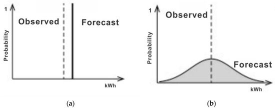
Figure 1.
Comparison between (a) deterministic and (b) probabilistic forecast models.
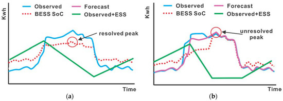
Figure 2.
Deterministic forecast and battery energy-storage systems BESS schedule analysis (a) when forecast coincides with observed (b) when observed deviates from the forecast.
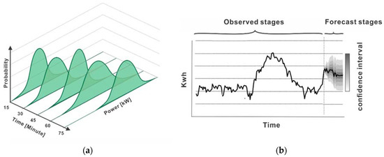
Figure 3.
(a) Demand forecast as a probability distribution (DPD); (b) Demand distribution forecast with confidence interval.
As depicted in Figure 3b, the probability distribution is generally narrow at the beginning of the forecast stages and becomes wider as it gets farther from the current moment. This phenomenon calls for re-forecasting to restore confidence in the forecast. In dynamic-interval forecasting, the forecast is performed multiple times in a day horizon in order to restore confidence in the forecast. The notion is to forecast at wider intervals during the demand off-peak period and narrow intervals during demand peak periods. DIDF helps track the forecasted distribution with high accuracy because the confidence interval of the forecast is improved in the next forecast interval.
2.2. Dimensionality Reduction Module
Because of the stochastic nature of the input data, many demand profile scenarios are possible. For example, given demand distribution samples at 15-min intervals in a day horizon, there are n = 96 sample points, where n is the number of demand distributions in a day horizon. The number of possible demand profile scenarios that can arise from this setup is , where a is the number of samples in each demand distribution. If there are a = 5 samples in each demand distribution, the number of possible demand profile scenarios can be evaluated as , which is not feasible for real-time optimization even with a high-performance computer. A Monte Carlo simulation can be used to select plausible scenarios to follow the original demand distribution for a representational selection. However, the number of scenarios to select is a trade-off between accuracy and computational complexity. In real-time applications, time is of the essence; therefore, using dense or high-dimensional data will affect the execution time. From this perspective, it is prudent to perform dimensionality reduction of the data with high fidelity.
2.2.1. Time-Of-Use (TOU) Partitioning
This paper proposes a method to reduce the dimension of DPD to improve the computational time of the optimization algorithm.
To reduce the dimension of the DPD two conditions are satisfied:
- Obtain the value of dimension reduction
- Accurate TOU Pricing: the objective of the stochastic optimization is to minimize electric cost, the electric cost in turn depends on TOU price which varies depending on the time of day. Figure 1 represents TOU policy of the Korean electric power company (KEPCO) which shows the different periods (partitions) in a day horizon with different time of use prices. The price changes are different depending on the day of the week and season [26]. Periods marked red have the highest price tag, followed by the yellow periods, with the green periods having the lowest price tag.
Based on the first condition, DPD of dimension is reduced to dimension where is the original dimension of the DPD and is the dimension to reduce for a faster computational time while maintaining an appreciable level of accuracy ().
The constraint in the second condition is to ensure the reduce dimension ties in with given TOU pricing interval for an accurate electric cost evaluation. To fulfill this, the minimum possible value that can take in order to satisfy the TOU constraint is defined as w. If some demand values will be misclassified into wrong TOU horizons during the reduction process, thereby attracting a wrong TOU price. As such, . As shown in Figure 4, a day horizon is partitioned into different pricing periods. The number of pricing periods in a day horizon as a result of TOU is defined as , different days in a season have different pricing periods. From Figure 4 can take on values of depending on the day of the week and season. represents the number of partitions for Sundays in all seasons, represents the number of partitions for Saturdays in all seasons, represents the number of partitions for weekdays in spring or fall, and represents the number of partitions for weekdays in winter or summer. Considering all days in every season, the maximum value that can take on should be the minimum values that can take to satisfy the TOU pricing constraint (i.e., ). One caveat that needs to be taken care of is days where . When or a parameter is introduced to pad to make up to . can be evaluated using (1).
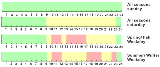
Figure 4.
KEPCO time-of-use (TOU) daily partitions.
2.2.2. Piecewise Peak Approximation
Given a probability distribution forecast of demand, referred to as DPD, , where is the probability distribution forecasted at the i-th time instance, piecewise peak approximation (PPA) is performed.
To proceed with PPA, a day horizon is divided into partitions to following TOU. From Figure 5, the red dashed line is the peak limit which is defined for each distribution in DPD. The peak propensity (probability to exceed the peak limit) for each distribution in DPD is evaluated using (2). The reduction is achieved by approximating all distributions found in a partition with the distribution having the maximum peak propensity (3).
where is the probability function, is the peak limit.
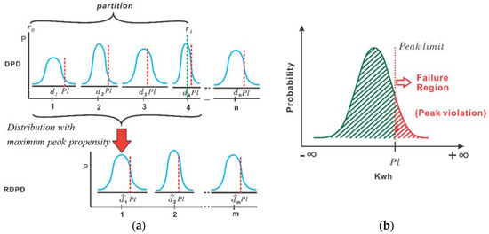
Figure 5.
(a) Converting distributions in a partition distribution to a single distribution using piecewise peak approximation (PPA) (b) Peak propensity or failure region of demand distribution.
The most common measure of central tendency used for such approximations is the average, as used in the deterministic case in [27,28]. This idea is also applicable in a stochastic case. However, since the peaking value is of the essence, using the average of demand distributions that fall under a partition could compromise the peak information. To carry the peaking feature, the distributions in a partition are approximated as the distribution with the maximum peak propensity, as illustrated in Figure 5a,b. The PPA produces a reduced demand probability distribution (RDPD) represented as , where is the distribution with the maximum peak propensity in the k-th partition, marks the beginning of the (k + 1)-th partition and end of the k-th partition, with . corresponds to potential points where TOU pricing changes occur. Preserving these price-change points during dimensionality reduction makes it convenient to apply the right TOU price during optimization.
Algorithm 1 describes the PPA process.
| Algorithm 1. PPA (). |
| begin 1. 2. 3. for i = 1 to c 4. 5. Endfor 6. for each partition in Z,k 7. 8. 9. Endfor end |
2.3. Stochastic Optimization
Stochastic programming is an approach for modelling optimization problems that involve uncertainty. Whereas deterministic optimization problems are formulated with known parameters, real-world problems almost invariably include parameters which are unknown at the time a decision should be made. When the parameters are uncertain but assumed to lie in some given set of possible values, one might seek a solution that is feasible for all possible parameter choices and optimizes a given objective function [25].
Stochastic optimization approaches the demand side management (DSM) problem by optimizing (minimizing) the total cost on average, , where x is the decision variable and D is demand as a random variable. Stochastic optimization evaluates the best cost and controls the peak demand for a given objective under demand uncertainties.
3. Problem Formulation
The objective of the proposed approach is to provide demand side management considering demand uncertainties. The algorithm performs a probability distribution forecast at set intervals using empirical data. The demand probability distribution (DPD) produce after the forecast is dimensionally reduced for faster computation via piecewise peak approximation (PPA). The reduce demand probability distribution (RDPD) is used as input to the stochastic optimization in conjunction with energy tariff and parameter constraints which seeks a robust BESS schedule with a given objective while satisfying BESS’s technical and efficiency constraints, as shown in Figure 6. The objective function of the stochastic optimization is divided into two parts:
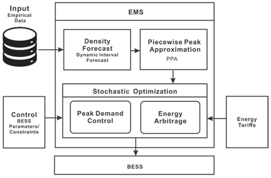
Figure 6.
Proposed system architecture.
- Energy Cost (TOU), which is computed at every time interval
- Demand (Peak) Cost, which is evaluated at the end of every month
3.1. Energy Cost
The energy cost represents the amount of energy used within a period multiplied by the TOU energy price. In a distribution sense, the energy cost is the total expected demand multiplied by the TOU energy price, which can be evaluated using (4).
where is the k-th distribution in RDPD, is the BESS schedule provided at the k-th instance by the optimization algorithm, is the TOU energy price at the k-th instance, is the expected demand of the k-th distribution in RDPD, and is the total expected cost of energy in a day.
3.2. Demand Cost
The demand cost is the maximum 15-min average power over a month multiplied by the demand price. This is evaluated using (6). The demand cost and energy cost must be unified. Normally, the demand cost is evaluated monthly, whereas the energy cost is calculated at a unit time interval. Because of this difference in units, the demand cost needs to be evaluated correctly at unit time intervals such that the accumulated demand cost over a month is equal to the monthly demand cost, as expressed by (10). The unified daily demand cost can be evaluated using (11).
where is demand price for a month, is the maximum demand on the l-th day, is maximum demand for a month, is the peak demand distribution at instance k on the l-th day, is the demand distribution at an instance k in RDPD on l-th day, Pl is the peak demand limit, P(.) is a probability function, is the unified demand price at any instance in a day, is the monthly demand cost, is the unified daily demand cost, q is the number of days in a month, with .
By KEPCO policy, the demand value used to evaluate demand cost is obtained using (9); thus, if the current recorded demand is greater than the Pl, the recorded demand value is used in calculating the cost. If the recorded demand is less than the Pl, the value of the Pl is used to compute the cost. This is evaluated to achieve peak demand control.
3.3. Optimization
The objective function of the stochastic optimization is formulated as the ensemble of energy cost and demand cost (EC) (14). The design optimization algorithm provides BESS control schedule candidates at each iteration of the optimization process, , based on conditions established as constraints to the objective function, where is the x-th BESS control schedule, is the BESS value scheduled at the kth instance in , , s is the number of iterations via the optimization algorithm.
For each , the ensemble of energy cost and demand cost is evaluated; this is evaluated as the minimum of both parameters. This is repeated for each iteration of the BESS control sequences until the one with the least cost on average is found. The objective function for the stochastic optimization is formulated as (16).
An inequality constraint is imposed on the objective function such that the state of the charge (SOC) of the BESS at the beginning of a day should be the same as that at the end of the day (17). Furthermore, the SOC of the BESS should be in the range of and , thus maximum and minimum SOC, respectively, as expressed by (18).
where is the SOC at instance k; and are the initial and final SOC, respectively, is the efficiency of BESS, and are the charge and discharge efficiency, respectively, and is the BESS capacity. The constraints guarantee that the optimization returns feasible solutions.
4. Case Study
In this section, the proposed approach is implemented with a case study and simulated for results. For the case study, 2016 and 2017 data from a real-site in South Korean was obtained. The data is recorded at an interval of 15 min in a day horizon, because of KEPCO’s policy of recording peak demand in 15-min intervals. The 2016 data is used for the daily interval forecast for 2017. The 2017 forecast data is used to implement the DSM algorithm, and the observed data is used for testing and for result analysis.
By convenience, a density forecast of 250 elements per each distribution is used. Dynamic-interval density forecast (DIDF) is performed following TOU partitions in a day horizon to obtain demand probability distribution (DPD). DPD of n dimensional space is reduced to m dimensional space which is referred to as a reduced reduce demand probability distribution (RDPD) via PPA for stochastic optimization. During peak times, the forecast is performed after every 15-min interval, whereas at off-peak times, the forecast is made on the order of hour intervals, followed by 2 h, 3 h, etc., depending on the size of the off-peak interval. Stochastic optimization is performed using RDPD. Particle-swarm optimization (PSO) [29] with a swarm size of 500, inertia of 0.6, and desired accuracy of 1 × 10⁻¹⁰ is used to implement the stochastic optimization procedure using the parameters in Table 1 at intervals following DIDF. TOU pricing is based on data from KEPCO [26].

Table 1.
Simulation parameters.
Table 1 shows the parameters used for the case study. The simulation was realized in MATLAB 2014 on an Intel i5 processor with 16 GB of RAM. On average, it takes 55 s to complete a single run of the stochastic optimization.
Figure 7 and Figure 8 present the results of the robust BESS schedule as applied to the expected demand. The results also show a comparison of the expected demand under the BESS schedule as well as when the BESS is absent. Each figure presents the expected demand, SOC of BESS, as well as the cost of expected demand when the BESS schedule is applied and when it is not. At the beginning of the day, BESS starts operation from the minimum SOC value, and the same value is maintained at the end of the day. The optimal BESS schedule obtained after stochastic optimization is verified against the most probable demand of the distribution. Figure 7a presents a stochastic optimization algorithm considering only energy arbitrage. It can be observed that the BESS discharges heavily during the critical TOU periods (peak times), indicated by the red band because the TOU price is high during this period. As such, it discharges prior to charging to full capacity during the off-peak period, in which TOU price is cheaper. Figure 7b shows the result where the algorithm considers only the peak demand cost. Figure 8 presents the results where the algorithm considers both the peak demand cost and energy arbitrage. In Figure 7b and Figure 8, the BESS schedule discharges heavily during the peak periods from 10 a.m. to 2 p.m. to resolve the demand peak exceeding the peak limit.
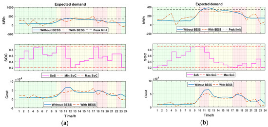
Figure 7.
(a) Demand side management (DSM) algorithm results considering only energy arbitrage (b) DSM algorithm results considering only peak demand control.
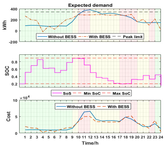
Figure 8.
DSM algorithm results considering energy arbitrage and peak demand control.
From Table 2, it can be observed that implementing the algorithm considering only energy arbitrage cost performs poorly in terms of peak reduction, but it is the best in terms of cost reduction. This is because it seeks only to reduce cost and not peak demand. With a previous peak value of 1763 kW, the algorithm causes a new peak of 2072 kW, representing an 18% increment in peak. In contrast, it provides the best yearly cost reduction of ₩35,296,338 in 2017. When the algorithm features only peak control, it is able to reduce the peak from 1763 kW to 1330 kW, which is a peak reduction of 26% and a yearly cost reduction of ₩2,937,306.
Table 2.
Simulation results.
An ensemble of energy arbitrage and peak control seeks to harness the benefit of the two algorithms; as such, the results show a reduction of 1308 kW in peak, representing a 26% decrease and a yearly cost reduction of ₩9,636,600.
Although implementing energy arbitrage alone provides the best energy cost, it also results in the worst peak control. The peak control case also has a good peak demand reduction, but also the worst yearly cost reduction. A combination of the two presents a compromise between these two factors to achieve a better cost and the best cost reduction.
5. Discussion
The proposed demand side management algorithm is compared with a deterministic optimization (DO) method using a deterministic day ahead forecast which is predominantly proposed in other research. The deterministic approach forecasts a day ahead demand profile which is used to evaluate an optimal BESS schedule for the next day, as shown in Figure 9a.
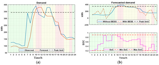
Figure 9.
(a) Day ahead forecast and observed demand; (b) BESS schedule on forecasted demand using deterministic optimization (DO).
Figure 9b shows the forecasted demand and the effect of the subsequent BESS schedule that was generated from the optimization algorithm. From the figure, it can be observed that although the peak demand is reduced, the reduction strictly follows the peak limit. The peak is reduced from 1518 kW to 1370 kW, representing a 9.8% reduction.
Figure 10a shows the results of the BESS schedule obtained from the optimization algorithm as applied to the observed demand. It can be observed that the BESS schedule generated fails to reduce the peak demand because of inaccuracies in the forecast as compared to the observed demand. The BESS schedule rather increases the peak from 1563 kW to 1624 kW, representing a 3.8 increase in peak demand.
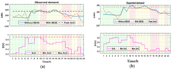
Figure 10.
(a) BESS schedule on observed demand using DO (b) BESS schedule on observed demand using proposed approach.
Figure 10b shows the results when the proposed real-time demand side management solution is applied to the observed demand. It can be observed that the real time algorithms perform better, since the dynamic interval density forecast reforecast the demand at set intervals to correct the deviation in the forecast. This approach is able to reduce the peak demand from 1563 kW to 1236 kW representing a 20.9% reduction.
6. Conclusions
This paper has proposed a DSM solution that incorporates a dynamic interval density forecast with a piecewise peak approximation for stochastic optimization.
The DSM solution has been verified using demand data from a real industrial site in South Korea. The results show that energy arbitrage alone cannot reduce the peak demand. In the case where the algorithm implements only energy arbitrage, a peak increase of 18% was incurred. When the algorithm implements an ensemble of energy arbitrage and peak demand cost, the peak demand is reduced by 26%. Unlike the deterministic case, where the forecast is performed once in a day horizon, the proposed solution performs the forecast at set intervals in a day horizon to restore confidence in the forecast should it deviate. This ensures a much more accurate forecast and a robust BESS schedule. For verification, the proposed demand side management algorithm is compared to a deterministic algorithm; the proposed method achieves 20.9% in peak reduction while the deterministic case achieves 9.8%. This real-time algorithm is applicable to industrial or commercial settings.
Author Contributions
S.H. conceived and supervised the work. M.A.A. designed and performed the experiments and wrote the paper. D.K. proof read the paper.
Acknowledgments
This work was supported by Korea Electric Power Research Institute (KEPRI) belonging to Korea Electric Power Corporation (KEPCO) for the project no. R16DA01.
Conflicts of Interest
The authors declare no conflict of interest.
References
- Gelazanskas, L.; Gamage, K.A.A. Demand side management in smart grid: A review and proposals for future direction. Sustain. Cities Soc. 2014, 11, 22–30. [Google Scholar] [CrossRef]
- Rahmani-Andebili, M. Nonlinear demand response programs for residential customers with nonlinear behavioral models. Energy Build. 2016, 119, 352–362. [Google Scholar] [CrossRef]
- Palensky, P.; Dietrich, D. Demand side management: Demand response, intelligent energy systems, and smart loads. IEEE Trans. Ind. Inform. 2011, 7, 381–388. [Google Scholar] [CrossRef]
- Logenthiran, T.; Srinivasan, D.; Shun, T.Z. Demand side management in smart grid using heuristic optimization. IEEE Trans. Smart Grid 2012, 3, 1244–1252. [Google Scholar] [CrossRef]
- Ipakchi, A.; Albuyeh, F. Grid of the future. IEEE Power Energy Mag. 2009, 7, 52–62. [Google Scholar] [CrossRef]
- Liu, W.; Niu, S.; Xu, H. Optimal planning of battery energy storage considering reliability benefit and operation strategy in active distribution system. J. Mod. Power Syst. Clean Energy 2017, 5, 177–186. [Google Scholar] [CrossRef]
- Akhil, A.A.; Huff, G.; Currier, A.B.; Kaun, B.C.; Rastler, D.M.; Chen, S.B.; Cotter, A.L.; Bradshaw, D.T.; Gauntlett, W.D. DOE/EPRI Electricity Storage Handbook; United States National Nuclear Security Administration: Washington, DC, USA, 2015. [Google Scholar]
- Tsekouras, G.J.; Kanellos, F.D.; Mastorakis, N. Computational Problems in Science and Engineering; Springer: Berlin, Germany, 2015; Volume 343, pp. 19–59. [Google Scholar]
- Aneiros, G.; Vilar, J.; Raña, P. Short-term forecast of daily curves of electricity demand and price. Int. J. Electr. Power Energy Syst. 2016, 80, 96–108. [Google Scholar] [CrossRef]
- Khan, G.M.; Khan, S.; Ullah, F. Short-term daily peak load forecasting using fast learning neural network. In Proceedings of the 2011 11th International Conference on Intelligent Systems Design and Applications, Cordoba, Spain, 22–24 November 2011; pp. 843–848. [Google Scholar]
- Dash, P.K.; Satpathy, H.P.; Liew, A.C. A real-time short-term peak and average load forecasting system using a self-organising fuzzy neural network. Eng. Appl. Artif. Intell. 1998, 11, 307–316. [Google Scholar] [CrossRef]
- Feinberg, E.A.; Genethliou, D. Peak demand control in commercial buildings with target peak adjustment based on load forecasting. Appl. Math. Power Syst. 2005, 2, 269–285. [Google Scholar]
- Dabbagh, M.; Hamdaoui, B.; Rayes, A.; Guizani, M. Shaving Data Center Power Demand Peaks through Energy Storage and Workload Shifting Control. IEEE Trans. Cloud Comput. 2017. [Google Scholar] [CrossRef]
- Lin, Q.; Yin, M.; Shi, D.; Qu, H. Optimal Control of Battery Energy Storage System Integrated in PV Station Considering Peak Shaving. Chin. Autom. Congr. (CAC) 2017, 2017, 2750–2754. [Google Scholar]
- Lu, C.; Xu, H.; Pan, X.; Song, J. Optimal sizing and control of battery energy storage system for peak load shaving. Energies 2014, 7, 8396–8410. [Google Scholar] [CrossRef]
- Cho, K.; Kim, S.; Kim, J.; Kim, E.; Kim, Y.; Cho, C. Optimal ESS Scheduling considering Demand Response for Electricity Charge Minimization under Time of Use Price Key words. Renew. Energy Power Qual. J. 2016, 264–267. [Google Scholar] [CrossRef]
- Elizabeth, F.Q.; Nghiem, T.X.; Behl, M.; Mangharam, R.; Pappas, G.J. Scalable Scheduling of Building Control Systems for Peak Demand Reduction. Am. Control Conf. 2012, 3050–3055. [Google Scholar] [CrossRef]
- Nghiem, T.X.; Behl, M.; Mangharam, R.; Pappas, G.J. Green scheduling of control systems for peak demand reduction. In Proceedings of the 2011 50th IEEE Conference on Decision and Control and European Control Conference (CDC-ECC), Orlando, FL, USA, 12–15 December 2011; pp. 5131–5136. [Google Scholar]
- Carpinelli, G.; Khormali, S.; Mottola, F.; Proto, D. Optimal operation of electrical energy storage systems for industrial applications. IEEE Power Energy Soc. Gen. Meet. 2013, 7, 1–5. [Google Scholar]
- Carpinelli, G.; Celli, G.; Mocci, S.; Mottola, F.; Pilo, F.; Proto, D. Optimal Integration of Distributed Energy Storage Devices in Smart Grids. IEEE Trans. Smart Grid 2013, 4, 985–995. [Google Scholar] [CrossRef]
- Chiodo, E.; Lauria, D. Probabilistic description and prediction of electric peak power demand. In Proceedings of the Electrical Systems for Aircraft, Railway and Ship Propulsion (ESARS), Bologna, Italy, 16–18 October 2012. [Google Scholar]
- Rahmani-Andebili, M.; Venayagamoorthy, G.K. Stochastic optimization for combined economic and emission dispatch with renewables. In Proceedings of the 2015 IEEE Symposium Series on Computational Intelligence, Cape Town, South Africa, 7–10 December 2015; pp. 1252–1258. [Google Scholar]
- Wang, Y.; Wang, B.; Zhang, T.; Nazaripouya, H.; Chu, C.C.; Gadh, R. Optimal energy management for Microgrid with stationary and mobile storages. In Proceedings of the IEEE Power Engineering Society Transmission and Distribution Conference, Dallas, TX, USA, 2–5 May 2016. [Google Scholar]
- Yudong, M.; Matuško, J.; Borrelli, F. Stochastic Model Predictive Control for Building HVAC Systems: Complexity and Conservatism. IEEE Trans. Control Syst. Technol. 2015, 23, 101–116. [Google Scholar]
- Shapiro, A.; Philpott, A. A Tutorial on Stochastic Programming. 2007, pp. 1–35. Available online: http://stoprog.org/stoprog/SPTutorial/TutorialSP.pdf (accessed on 3 April 2018).
- June, S.; Mar, S. Korea Electric Power Corporation Tariff. 2013. Available online: https://cyber.kepco.co.kr/kepco/EN/F/htmlView/ENFBHP00101.do?menuCd=EN060201. (accessed on 3 April 2018).
- Keogh, E.; Chakrabarti, K.; Pazzani, M.; Mehrotra, S. Dimensionality Reduction for Fast Similarity Search in Large Time Series Databases. Knowl. Inf. Syst. 2001, 3, 263–286. [Google Scholar] [CrossRef]
- Chakrabarti, K.; Keogh, E.; Mehrotra, S.; Pazzani, M. Locally adaptive dimensionality reduction for indexing large time series databases. ACM Trans. Database Syst. 2002, 27, 188–228. [Google Scholar] [CrossRef]
- Kennedy, J.; Eberhart, R. Particle swarm optimization. In Proceedings of the IEEE International Conference on Neural Networks, Perth, Australia, 27 November–1 December 1995; Volume 4, pp. 1942–1948. [Google Scholar]
© 2018 by the authors. Licensee MDPI, Basel, Switzerland. This article is an open access article distributed under the terms and conditions of the Creative Commons Attribution (CC BY) license (http://creativecommons.org/licenses/by/4.0/).