Experimental Study and Modeling of Ground-Source Heat Pumps with Combi-Storage in Buildings

Abstract

There is a continuous growth of heat pump installations in residential buildings in Germany. The heat pumps are not only used for space heating and domestic hot water consumption but also to offer flexibility to the grid. The high coefficient of performance and the low cost of heat storages made the heat pumps one of the optimal candidates for the power to heat applications. Thus, several questions are raised about the optimal integration and control of heat pump system with buffer storages to maximize its operation efficiency and minimize the operation costs. In this paper, an experimental investigation is performed to study the performance of a ground source heat pump (GSHP) with a combi-storage under several configurations and control factors. The experiments were performed on an innovative modular testbed that is capable of emulating a ground source to provide the heat pump with different temperature levels at different times of the day. Moreover, it can emulate the different building loads such as the space heating load and the domestic hot water consumption in real-time. The data gathered from the testbed and different experimental studies were used to develop a simulation model based on Modelica that can accurately simulate the dynamics of a GSHP in a building. The model was validated based on different metrics. Energetically, the difference between the developed model and the measured values was only 3% and 4% for the heat generation and electricity consumption, respectively.

1. Introduction

In German power sector, an ongoing increase of renewable energy integration can be witnessed. In 2016, 29% of gross generated electricity was produced from renewable energy sources (RES), which represents 192 TWh [1]. Such increase in the RESs integration is empowered by several policies such as the renewable energy act (EEG) [2]. The act guarantees the generator a fixed price over a specific term, which gives a priority to the RES in the electricity market. Having such weather dependent fluctuating RES in the market, raised the demand for flexibility to balance the generation. Sector coupling presented one way to mitigate the fluctuating RES and offer flexibility to the grid. Hence, it is receiving continuous attention not only within the research communities but also on the political and industrial level. Coupling the power to the heat sector is seen as one of the most influential and attractive approaches to decarbonize the heat sector and gain additional flexibility in power grid [3]. Considering that the consumed heat energy in Germany within different sectors was 1373 TWh in 2016 [4], there is a substantial room for power to heat application integration. An advantage of such applications is its attractive costs due to its dependency on heat storage that has significantly lower costs compared to batteries.

The heat pump is a major role player in sector coupling due to the progressive improvement of the coefficient of performance (COP) [5]. Hence, the number of heat pumps installations are on continuous growth on yearly basis, especially in the residential sector. According to [6], the heat pump installations in new buildings in 2016 reached 31.8%. Heat pump represents 34% of the market share of the single-family houses, 16% of the multi-family houses and 13.6% of the non-residential buildings. Ground-source heat pumps (GSHP), market is expected to be largely integrated in the zero emission buildings (ZEBs). According to [7,8], GSHP has a low operating cost, no outdoor units, longer life, and a higher CO${}_2$ emissions reduction. Moreover, the high efficiency of the GSHP is expected to minimize the required photovoltaic installation area and consequently minimizes the costs of the ZEBs.

The topics discussed within the literature covered large scope such as the thermodynamic cycle and compressor optimizations [9,10,11,12] hydraulic system configurations [13], performance evaluation [14,15], and integration in district heating and smart grids [5,16]. The research presented can be divided into experimental studies and numerical studies. The experimental studies were mostly oriented towards cycle and components optimization of the heat pumps. In [17], a carbon dioxide direct-expansion heat pump was investigated in different operating conditions. Yang et al. [18] studied the performance of solar ground source heat pump in dual heat source coupling modes to optimize the average system COP. Furthermore, Liu et al. [19] experimentally tested a gas engine driven heat pump for different operation modes. The author developed a prototype to test the heating and cooling performance for different evaporator’s inlet temperatures, ambient temperatures, and gas engine speeds. The numerical studies and simulations were utilized, where experimental studies would be costly. In [20], a heat pump was simulated to cover the load of a multi-zone office building. While in [21], a simulation model was developed to analyze the flow pumping of ground source heat pumps. Naldi et al. [22] developed a numerical model for a reversible multi-function heat pump to evaluate its performance in summer for domestic hot water (DHW) and space cooling. The numerical model was then evaluated against a model in TRNSYS.

In the residential sector, several studies were performed on GSHPs. The presented studies were mostly numerical. Also, it is oriented towards optimizing the heat pump control, system dimension and hydraulics to minimize the operation costs and maximize the use of renewable energies within the residential building as in [23,24,25,26,27]. Although numerical studies can provide relatively proper indicator of the behavior of a system, it is exposed to several uncertainties and its accuracy is always questioned, especially if the studied object is a thermodynamic system. Studies analyzing large models on the district level or micro grid levels have mostly 1-h resolution as in the review of [3], consequently, all dynamics of the heat pump systems are concealed. Moreover, in several cases, the COP is assumed to be constant and all the nonlinearities are ignored so that the optimization problem can converge faster. Yet, this exposes the model to inevitable uncertainties. On the building level, dynamic systems simulation programs are used such as TRNSYS or Modelica-based software as Simulation X [28]. These programs can detail the dynamics of the systems, yet as discussed in [29], their calibration is complicated. Moreover, these models are mostly validated by a plausibility check. Few research presented models, which were validated based on experimental results such as [8,30,31]. In [8], a simplified model was validated based on the maximum absolute mean deviation of the COP, thermal power and condenser water temperature. In [31], a black-box model was validated based on the root mean square deviation of the monthly efficiency. To evaluate properly a heat pump model, a detailed analysis of the energy generation and consumption, and system dynamics has to be performed. The energetic analysis can suffice for models looking forward to heat pump performance estimation, but dynamics analysis is a necessity for heat pump models integration in building models. Field tests were also performed to investigate installed heat pump systems [14]. These studies can provide a realistic investigation of the performance of heat pumps in general and a good indicator of the factors influencing the operation of heat pumps, yet it does not offer the flexibility of an experimental system. In a field test, the system parameters are usually fixed. Thus, there is no room for experimenting, but rather monitoring and analyzing the current status of a system. An experimental setup enables varying different parameter to understand the system behavior in any custom configuration. Moreover, the investment in field tests usually minimize the measurement points, which can lead to concealing several details that can contribute to a better understanding of the system dynamics.

Objectives

To provide realistic, reliable results, numerical studies have to be always supported by experimental results. Otherwise, any presented control system, mathematical model, or simulation model might be exposed to imminent uncertainties. In this paper, an experimental study is performed to validate a numerical model and present the optimal control requirements for a GSHP in a residential building. The experimental study does not only include a residential, commercial heat pump and combi-buffer storage but also a building load emulator to integrate the real space heating (SH) and DHW load of a building. The objectives of this paper can be summarized in the following:

• Presenting a novel modular heat pump testbed design that emulates a complete residential house. It includes a ground-source emulator, combi-buffer heat storage, and a building load emulator. The testbed is designed to be integrated with different heat pump types and hydraulic connections so that it can be used for standardization applications, control and optimization methods performance testing, and models validation
• Based on multiple experimental testing, the real-life optimal control criteria for a commercial, residential GSHP under the given constraints of the heat pumps manufactures have been identified.
• Demonstrating a Modelica-based heat pump model that can be easily integrated into building and district simulations due to its minimal computational requirements. The model was also validated and calibrated based on the experimental data of the presented testbed.

The structure of this paper is as follows: Section 2 describes the design and components of the testbed. Moreover, it introduces the measurements system used and discusses the testbed control dynamics. Section 3 presents the experimental testing procedure and its purpose. Section 4 presents the validated Modelica heat pump model and its structure. Section 5 discusses the results of the experimental testing and the validation of the Modelica model. Section 6 presents a conclusive summary of the experimental study and the model performance.

2. Experimental System Description

2.1. Overview

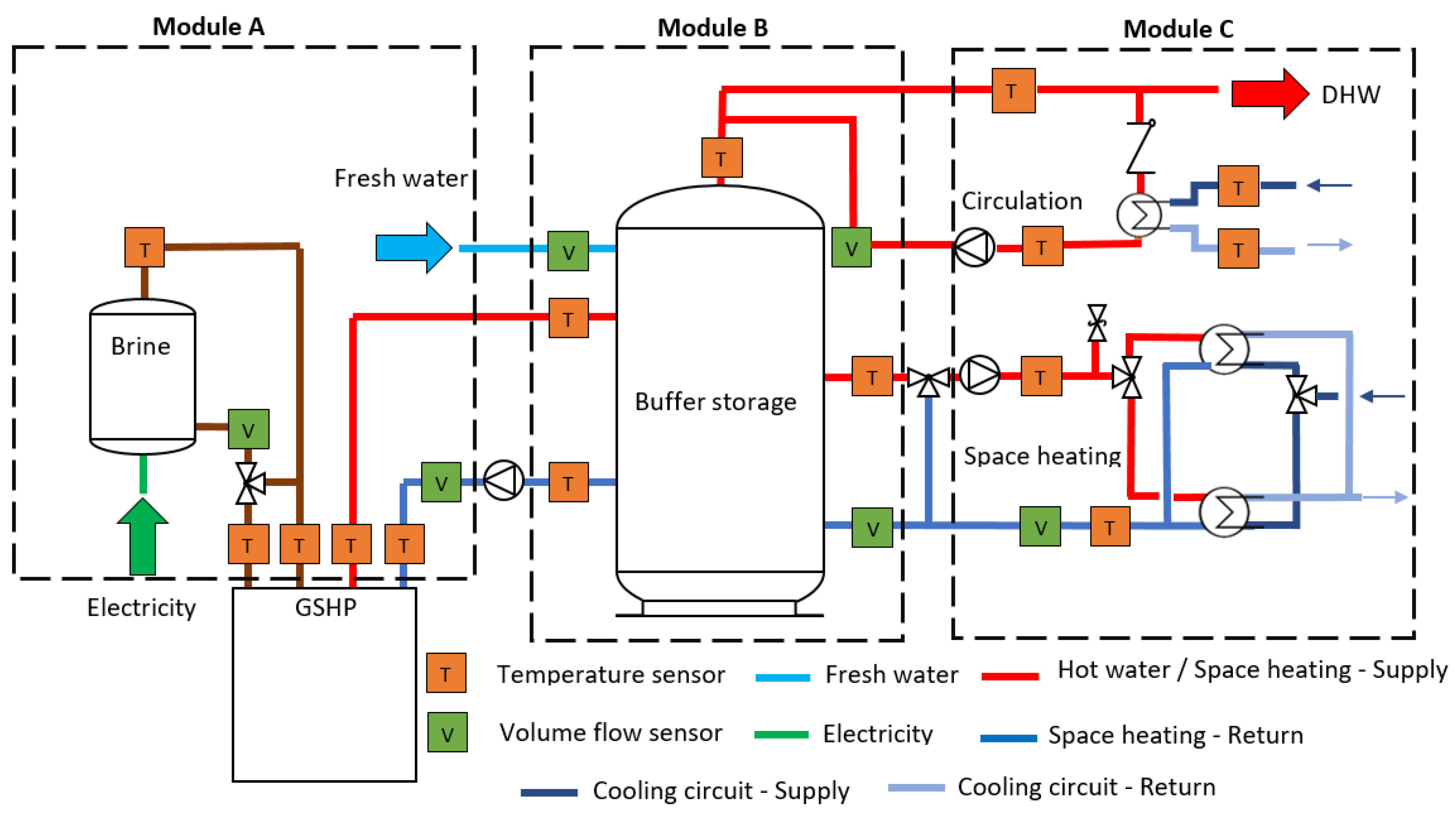
The testbed consists of 3 different modules: ground-source emulator (A), combi-storage (B), and the building loads emulator (C). Figure 1 and Figure 2 show a simplified hydraulic scheme and the real testbed, respectively. The presented hydraulic configuration is not a permanent configuration, but rather the one used for the experiments documented in this paper. Other possible configuration can be also implemented such as a direct connection between the heat pump and module C, replacing module B with a DHW tank module, or having two separate modules for a DHW tank and a buffer tank. Each module has its independent control and measurement system to facilitate the integration of different modules. The GSHP used is a STIEBEL ELTRON WPF10 heat pump with a thermal power of 10.31 kW and a COP of 5.02 by B0/W35 according to the standard EN 14511. A brine pump and heating system circulation pump is already integrated within the GSHP. Moreover, the GSHP is also equipped with an emergency/backup electrical heater of 8.8 kW.

2.2. Module A: Ground-Source Emulator

Module A emulates a ground-source, which is equivalent to a controlled environment room for the ASHP. The module consists of 300-liter storage that is heated by a 12.5 kW electrical heater. This storage is filled with a water-glycol mixture as an anti-freezing heat transfer fluid. The electrical heater is controlled via a hysteresis regulator to maintain a maximum set-temperature for the whole tank of 40 ${}^{\circ }$C. The hysteresis limits can be adjusted based on the user settings. To deliver a specific temperature profile to the heat pump, a conventional SH mixer is used to mix the supply of the storage with the return of the heat pump till it reaches the required temperature. This types of mixers can lead to a slow reaction towards changes in the set points but provides a rather stable output as discussed later in Section 2.6.

2.3. Module B: Combi-Storage Module

This module represents one of the storage system configurations in a residential household. The storage system consists of a 749 l combi-hygienic buffer storage for SH and DHW consumption. The cold water is heated via a stainless steel heat exchanger that goes through the height of the tank to supply DHW. Furthermore, a coaxial pipe is inserted in this heat exchanger to enable DHW circulation and maintain proper hot water temperature in the pipes. An example of the coaxial pipe circulation connection can be presented in [32].

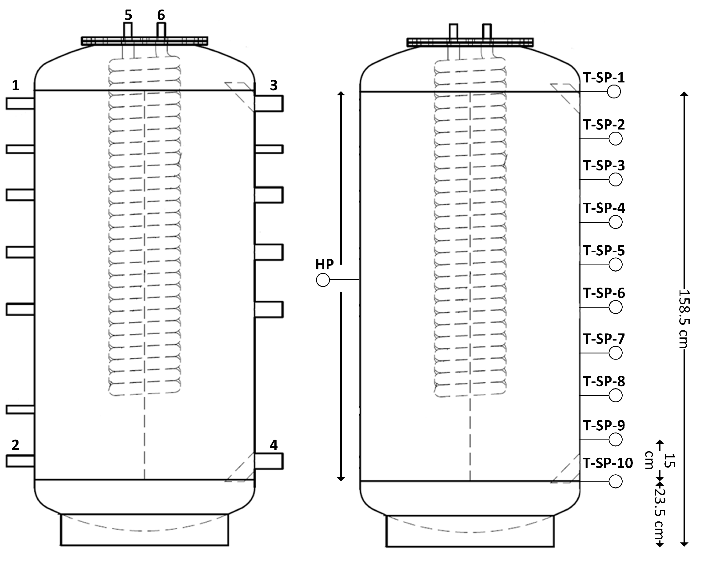
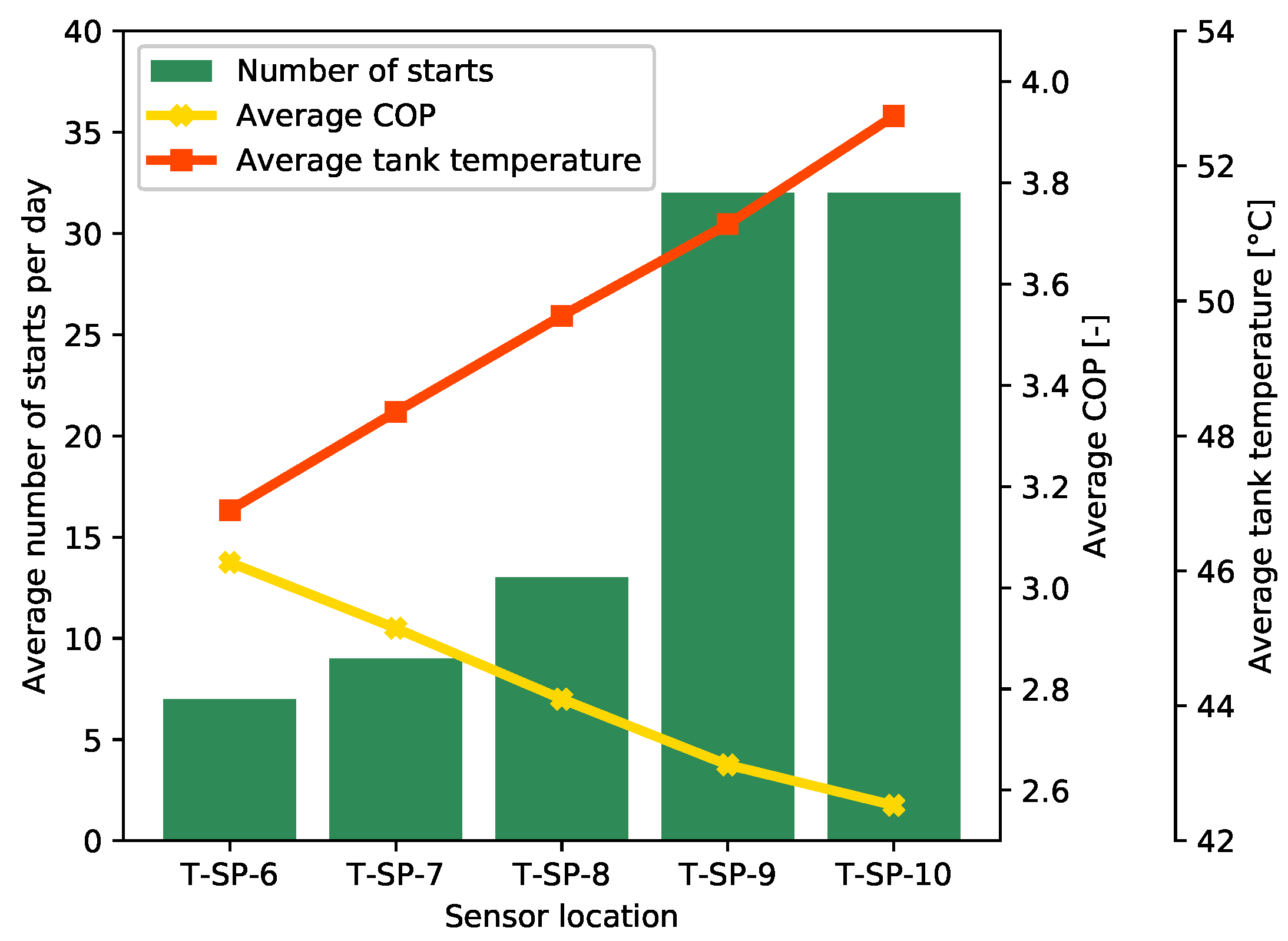
To assess the energetic content of the buffer storage over time, ten temperature sensors are placed over the length of the tank as shown in Figure 3. T-SP-1 refers to the sensor on the top of the tank, while T-SP-10 refers to the sensor at the bottom of the tank. The sensors are placed at equidistant distances of 15 cm. Through this sensors’ set, the energy at each layer of the tank as well as the overall tank content can be evaluated. This data represents a necessary input to the energy management systems (EMS) and control algorithms to decide on the load shifting potential and the available flexibility that can be offered to the grid. Further information about the storage management system can be found in [33]. On the left side of the tank, the heat pump buffer sensor, HP sensor, is installed. According to the installation manual of the heat pump, this sensor has to be placed at the bottom of the tank. Within this paper, the sensor position will vary to show its influence on the system performance as shown in Section 3.

Figure 3 shows as well the inlet and outlet pipes of the storage, where 1, 2, 3, 4, 5, and 6 are space heating supply, space heating return, heat pump supply, heat pump return, fresh water, and domestic hot water, respectively. Those inlets and outlets were chosen to maximize the stratification efficiency and avoid mixing within the tank.

2.4. Module C: Building Loads Emulator

This module is the most complicated as it has to represent the SH and DHW consumption of a household. The SH circuit consists of a mixer, as in Figure 1, that mixes the hot water supply of the tank with the return of the SH circuit to reach the required set temperature. The building heating load is then made present via using heat exchangers that are cooled via a cooling system. The flow rate of the cooling system is the one influencing the building load magnitude and defining the return temperature of the SH circuit. Such flow rate is controlled via a motor control valve that positions the valve according to the required set point. Within the SH circuit, two heat exchangers are available of different powers and capacities. One heat exchanger is dedicated to old building heating loads that can reach up to 20 kW and have a high flow rate, while the other one is only for new buildings with a maximum power of 7 kW. Two motor valves are used to switch between the two heat exchanger as per the testbed setup.

The hot water consumption is realized via three magnetic valves representing three different types of taps within the household. These valves can present various activities such as showering, washing, and cooking. The flow rate of the valves can be adjusted manually to match the standard flow rate of the activity. To show the effect of the hot water consumption on the heat storage, a household profile of hot water consumption can be delivered to the testbed. The opening and closing time and duration of the water tapping is defined for the different valves based on the given profile. Consequently, a similar energetic profile can be executed.

The DHW circulation pump is managing the circulation exactly as in a conventional household circulation pump. The pump can be switched on or off based on a circulation schedule or hot water temperature in the pipe. The circulated load is presented via a heat exchanger that is cooled via the cooling system, similar to the SH circuit heat exchanger. Such design was adopted for different testbeds in the labs of the Institute for energy economy and application technology (IfE) as shown in [35].

2.5. Measurement System

For the temperature measurements, four wire PT100 sensors are used. The sensors accuracy class is F0.15 (Class A) according to the DIN EN 60751, which means that the tolerance is $\pm (0.15+0.002|T\left|\right)$. Hence, for a temperature T of 65 ${}^{\circ }$C, the tolerance is ±0.28 ${}^{\circ }$C. To maximize the accuracy further, a temperature sensor calibration device of a higher accuracy was used.

Magnetic inductive flow measurements devices are used to measure the volume flow rate. The flow measurements devices were already calibrated by the manufacturer. Consequently, no additional calibration was performed. For the nominal flow rate, the error of the devices varied between 0.2% and 0.5% depending on the sensor type and the size of the pipe.

The electrical power of the heat pump is measured via a 3-phase electricity meter (KDK PRO 380) of class B accuracy, which is 1% according to the EN 50470-1/3. The meter is connected to the measurement system via MODBUS RTU connection, which communicates the power, currents, and voltages of the 3 phases each second.

The sensors and actuators of the whole testbed are connected to National Instruments (NI) compact reconfigurable IO (cRIO) chassis and modules that receive and send different digital or analog inputs and outputs. The control program and data logger are based on LabVIEW that runs on a conventional PC.

2.6. System and Control Dynamics

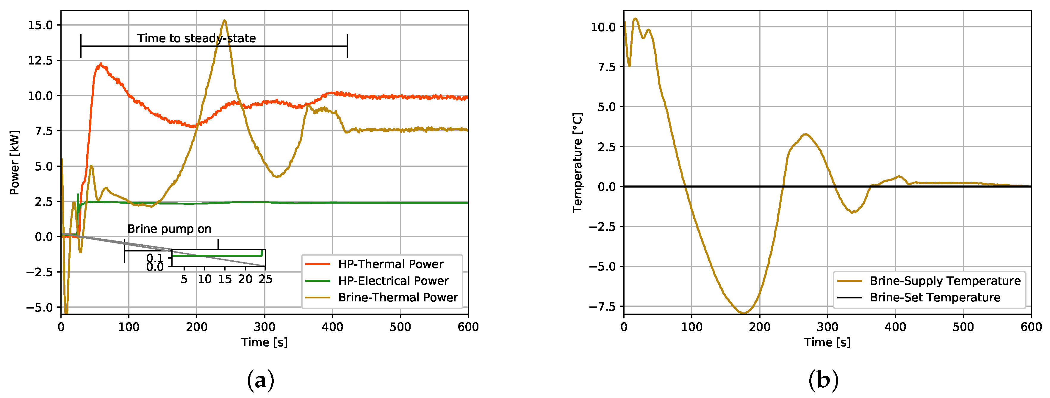
The main purpose of the testbed is to show the detailed dynamics of a heat pump system to be able to develop and validate a realistic numerical model. In Figure 4a, the start dynamics of the heat pump are shown. As soon as the heat pump starts, the brine pump operates for 24 s; then the compressor is switched on. It takes the testbed 393 s to reach the steady state due to the mixer control dynamics, yet it does not influence the thermal power of the heat pump significantly. The brine power fluctuations between 2.5 till 15.1 kW led only to variations of 10 ± 2.5 kW${}_{th}$, within those 393 s. The brine power represents the power supplied by the heat source. The mixer controller effect can be more clearly described in Figure 4b. For a set temperature of 0 ${}^{\circ }$C, the mixer started to mix the tank temperature with the return of the heat pump. Due to both of the start dynamics of the mixer supply and heat pump return, the fluctuations occurred within the time to steady state. Once a steady state is reached, the mixer controller can maintain the set temperature, while minimizing the fluctuations.

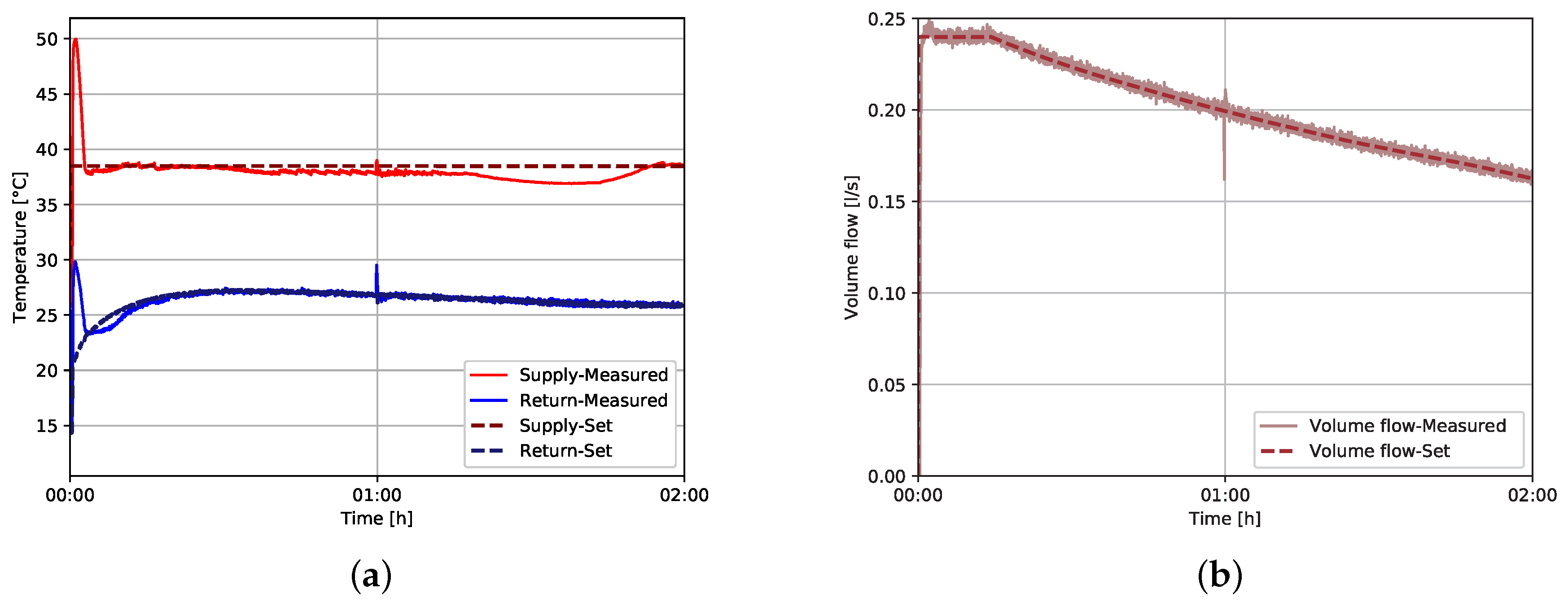
For the control system in module C, Figure 5 shows the control dynamics of the temperature of the flow rate. In Figure 5a, the measured and set heating circuit supply and return temperatures are plotted against two hours of time to show the system dynamics. The control tolerance of the supply temperature mixer is ±0.5 K, which is significantly better than the control in realistic buildings, where the tolerance reaches ±3 K. A smaller tolerance was required to accurately emulate a building load profile on the testbed. The return temperature was more accurately controlled as the motor valve has a continuous PID controller. Consequently, a tolerance of ±0.1 to ± 0.15 K was achieved, which is challenging considering the low inertia of the system (i.e., the water volume of the system is small compared to a real building).

The volume of the flow rate of the heating system circulation pump was also controlled via a PID controller. In Figure 5b, the measured set and measured flow rate are presented. It can be deduced that the pump and the controller were able to flow accurately the set point with a tolerance less than $0.01$ l/s. The graph was plotted against the same time of measurements of the supply and return temperature, to be able to show the dynamics of the two graphs simultaneously.

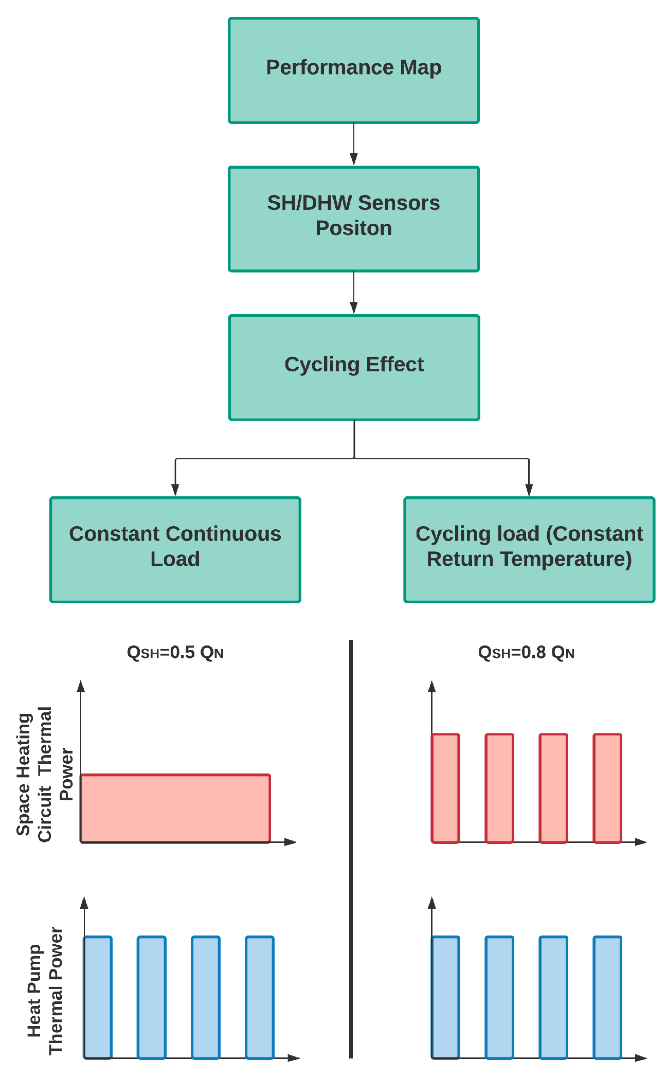
3. Experimental Testing Procedure

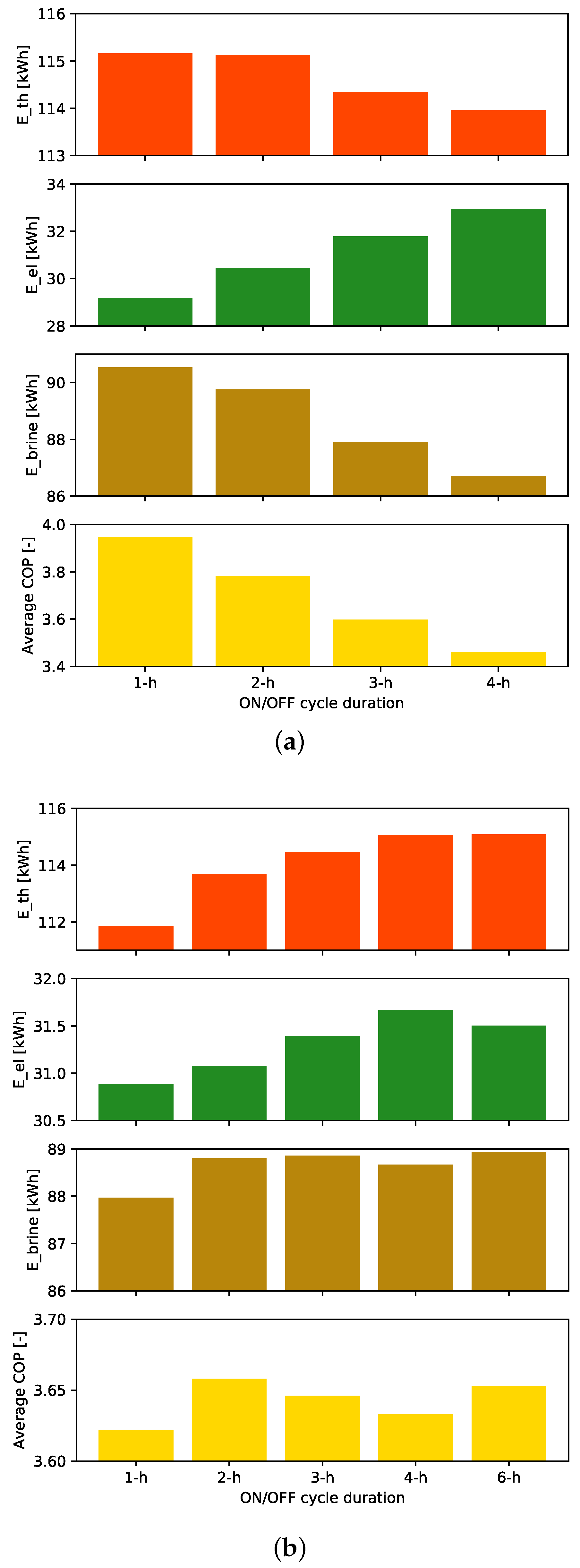
Four major experiments are covered within the scope of this paper, as in Figure 6. The first group of experiments is to define the performance map of the heat pump. This group of experiments analyzes the given heat pump performance under different heating supply temperature and brine temperatures. The second group of experiments investigates the optimal SH and DHW sensor position and reveals its effect on the overall system performance in buildings. In the third and fourth group of experiments, the optimal control rules for EMS are defined through testing the cycling effect. In a residential heat pump, the control parameters are limited to a boolean signal to switch the heat pump on or off. Consequently, an EMS in a residential building does not have any influence on other technical parameters such as the flow rate of brine pump or the controller of the heating circuit between the heat pump and the combi-storage. Based on these constrains, the heat pump optimal control rules can be defined. In cycling effect experiment with constant continuous load, the thermal load is given to the building emulator (e.g., 5 kW), constant through the whole 24 h, while heat pump had to cycle between on and off. Within this group of experiments, four experiments were performed with a duty cycle of 50%. The switching time was varied between 1, 2, 3, and 4 h. The 6 h duration was not performed in this experiment due to the limited thermal capacity of the combi-storage. To maintain the energy balance, the thermal load $Q_{SH}$ was limited to 50% of the nominal thermal power of the heat pump $Q_N$. Cycling effect was also tested while trying to maintain a constant return temperature. The $Q_{SH}$ was limited to 80% of $Q_N$. Due to the increase of $Q_{SH}$, the 6-h cycle was made possible. Thus, six experiments were performed, the 1, 2, 3, 4, 6 h cycles.

Through this set of experiments, the characteristic of the operation of the heat pump can be clarified, in addition to the impact of sensor installation position. Moreover, the results of the cycling effect experiments can provide a clear picture of the optimal control criteria of GSHP.

4. Modelica Based Model

According to [36], the heat pump modeling approaches into physical, black box and grey box approach. The physical approach can forecast the dynamic behavior of a system. Hence, it is often used for heat pump design and parameters optimization. Black boxes can be easily computed and are useful for large systems, yet it is usually concealing several system dynamics to maintain its simplicity. Grey box models try to achieve a balance between the two aforementioned approaches. For residential buildings modeling, three main criteria have to be satisfied:

• Simplicity: the model has to be easily computable as the building modeling software such as the Modelica and TRNSYS are not yet powerful enough to solve the equations of multiple complicated dynamic systems simultaneously
• Accuracy: the model has to minimize the uncertainties of the results
• Dynamics: the model should not be concealing the dynamic behavior of the heat pump under different operating conditions.

In this paper, a semi-empirical dynamic model is presented that was developed on Modelica. Figure 7 shows a view of the structure of the model in Modelica. It was designed such that it can be coupled with Open Modelica Libraries [37] or Simulation X “Green City” Package [38]. Consequently, the basic model components were designed based on an Open Modelica Library, yet a separable interface was included to connect to the “Green City” package. The simulated thermal power of the heat pump $Q_{sim}$ and the coefficient of performance $CO{P}_{sim}$ are calculated empirically based on the collected experiments performed in Section 3. The $Q_{sim}$ is calculated as a function of the brine $T_b$ and the heating supply temperature $T_s$ as in Equation (1). $CO{P}_{sim}$ is also evaluated based on those two inputs either directly from the experimental tabulated data or from the empirical equation given in Equation (2). This polynomial equation was formulated based on data fitting algorithm of the experimental data. The $R^2$ is 0.99, while the sum squared error and the root mean squared error is 0.1727 and 0.0759, respectively. The electrical power of the heat pump $P_{sim}$ is then simply calculated based on Equation (3).

$$Q_{sim}=f(T_b,T_s)$$

(1)

$$\begin{array}{c}CO{P}_{sim}=f(T_b,T_s)\\ CO{P}_{sim}=11.16+0.2488\times T_b-0.2282\times T_s-0.003031\times T_b{T}_s+0.001405\times T_s^2\end{array}$$

(2)

$$P_{sim}=\frac{Q_{sim}}{CO{P}_{sim}}$$

(3)

Although the powers and COP of the heat pump can be accurately calculated using the presented equation, these data will not be sufficient to present the system dynamics such system thermal losses, system inertia, operation time of the brine pump before the compressor starts, resting time between two consecutive starts, and time to full power. Consequently, the calculated full power from Equation (1) is given as a prescribed thermal power to a thermal pipe directly. This pipe represents the outlet pipe of the heat exchanger of the condenser. Between the pipe and the prescribed heat model, there is a thermal resistor that was empirically calibrated to present conduction losses. The inertia of the system is represented by a thermal capacitor that can be initialized based on the system water volume as in Equation (4), where $C_p$ is the specific heat capacity of water, $Vol$ is the internal water volume of the heat pump, $\rho$ is the density of water. The convection losses were modeled as shown in Figure 7, assuming that the room temperature is always fixed at a value of 18 ${}^{\circ }$C. The convection heat loss factor was also empirically estimated and set as fixed value throughout the whole simulation.

$$C=C_p\times Vol\times \rho$$

(4)

Through the presented model, the aforementioned criteria for heat pump modeling for building simulations can be satisfied without adding any additional complexity to the heat pump model. Adding any additional details such as modeling the thermodynamic cycle would not contribute to the quality of the results in this situation as these variables are not monitored within the study of the dynamic behavior of a building.

5. Results

5.1. Experimental Analysis

5.1.1. System Performance

As explained in Section 3, the initial phase of the experimental study is to analyze the performance map of the given heat pump. Figure 8a shows the behavior of the COP as a function of the supply temperature and the brine temperature. At each of the measured points of $T_b$ and $T_s$, the set points were held constant, and measurement was taken as an average of 40 min of operation to maintain a proper steady and accurate measurements. The set points are defined as a discrete set of integers such that $T_s\in \{35,40,45,50,55,60,65\}$ and $T_b\in \{-5,0,10,15,20\}$. In Figure 8a, the measurements at 65 ${}^{\circ }$C was eliminated, as the heat pump cannot operate at $T_b=-5$ ${}^{\circ }$C and $T_s=65$ ${}^{\circ }$C, simultaneously. As shown, the COP increases as the supply temperature decreases and the brine temperature increases. The range of the COP is quite wide between 1.6 and 8.0. This means that the costs of operation of the heat pump to generate 1 kWh of heat can reach up to 500% compared to the cost of the most optimal possible operation. Consequently, it is a must to supply the numerical models with an accurate measured data, otherwise building model can be exposed to high uncertainties.

Figure 8b,c show the electrical power consumption and thermal power generation against different supply temperature and brine temperature, respectively. It can be noticed that the electrical power is not influenced by the brine temperature as much as the supply temperature. For the same brine temperature of 0 ${}^{\circ }$C, the electrical power consumption can vary from 1.8 to 3.6 kW, depending on the supply temperature. On the other hands, the thermal power generation is more influenced by the brine temperature. Depending on the brine temperature, the thermal power can vary between 7 to 16 kW.

5.1.2. Sensors Position

System setup and configuration in the building also has a significant influence on the behavior of the COP of the heat pump. In the field study of [14], the impact of efficient planning and installation on the heat pump seasonal performance factor was investigated. The installation process does not only include hydraulic system but also the DWH and SH sensors positioning on the storage system. Although direct connection of the SH circuit to the buildings without any buffer storage can lead to the most optimal operation, buffer storages are necessary to offer flexibility as in [39]. In the literature, different research discussed the sensor position. In [13], different sensors positions along a combi-storage were tested based on a simulation model. It was found that as the distance increases between the DHW sensor and the SH zone, the number of starts per year decreases. In [28,40], it was stated that the DHW sensor has no influence on the performance of the heat pump, yet the higher the position the better. Moreover, the author stated that sensors at a lower position could help in decreasing the set temperature while maintaining comfort.

Within this experimental study, one sensor was set in different position across the combi-storage to analyze the behavior of the heat pump and the heat storage as well. This sensor is referred to as the HP sensor. Additional sensors connections to the control of the heat pump manufacturer were not possible. The set temperature of the sensor was adjusted to a fixed value of 50 ${}^{\circ }$C. On the brine side, a constant temperature of 0 ${}^{\circ }$C was maintained. Figure 9 shows the average number of starts, average COP and average tank temperature at different sensors positions. The average COP is calculated according to Equation (5), where $E_{th}$ and $E_{el}$ is the accumulated thermal and electrical energy within a defined period, respectively.

$$CO{P}_{Average}=\frac{E_{th}}{E_{el}}$$

(5)

The sensor positions on the x-axis can be clarified through Figure 9. For each sensor position, the measurement was repeated for three consecutive days, then the average of the three days was taken. At T-SP-10 and T-SP-9 which are the lowest two sensors, the value of the number of starts is similar and significantly higher than the rest of positions. This means that if a sensor has to be allocated at a lower position on the tank as per the theoretical studies, this zone (below T-SP-9) has to be ignored for sensors allocations. The lowest sections of the tank are the sections which are cooled immediately once the heat pump switches off. Having a sensor at this position means that the heat pump has to keep always the whole capacity of the storage at the set temperature. Thus, the heat pump will not be using the heat storage capacity to increase its resting time. As the sensor is positioned more towards the upper zone of the tank, the lower is the number of starts per day. This also means that the storage heat content decreases because the useful volume that is kept at the set temperature decreases as indicated in Equation (6) [41], where $A_s$ is cross-sectional area of the storage, $T_{set}$ is the required set temperature and $T_{storage}\left(h\right)$ is the temperature across the height of the storage h.

$$\begin{array}{c}{E}_{storage}=\rho \times C_p\times A_s\times {\int }_0^h(T_{storage}\left(h\right)-T_{set})dh\\ \forall T_{storage}\left(h\right)>T_{set}\end{array}$$

(6)

On the other hands, as the average tank temperature decreases, the average COP also linearly increases, which fits the behavior presented by the performance map in Figure 8a. Between T-SP-10 and T-SP-6, the average COP increased by 21.5%, which is a significant increase that influences the economics of the heat pump considering that no intelligent control algorithms were yet deployed. The direct correlation between the average COP and the average tank temperature shows that COP is solely dependent on the tank set temperature.

5.1.3. Cycling Influence on the System Performance

In the first experiment, as explained in Section 3, a constant continuous load is set for SH circuit, which is almost equal to 50% of the nominal heating power of the heat pump. Hence, the space heating load was set to $Q_{SH}=5.0$ kW. On the brine side, a constant temperature of 0 ${}^{\circ }$C was maintained. For the combi-storage, an initial heat content was set for all the experiments of 3 kWh. Figure 10a shows $E_{th}$, $E_{el}$, $E_{brine}$ and the average COP for 1-h on/off cycle till 4-h on/off cycle, where $E_{brine}$ is thermal energy extracted from the brine circuit. 1-h on/off cycle means that the number of starts per day is 12, where 4-h means three starts per day. A 6-h cycle was not performed in this case due to the limited storage capacity that does not enable the heat pump to charge the storage for six hours continuously. In this experiment, the highest average COP was achieved by the 1-h cycle. It can be noticed that the energy extracted from the brine circuit is the highest, while the electricity consumed is the lowest. The heat generated is almost constant. It has varied only between 113.85 kWh to 115.2.

Although 1-h cycle has the highest number of starts, it achieved the highest COP because it maintained the lowest possible tank temperature. Having the heat pump operating for four hours then stopping for four hours while having a constant demand from the SH circuit means that the heat pump has to heat the buffer storage to higher temperatures to satisfy the demand during the off (i.e., resting time). Although the 4-h cycle minimized the number of starts to only three times per day, it does not lead to an optimal, efficient operation. The average COP was lowered by 13%. The lower number of starts might increase the lifetime of the compressor, yet this is not a measurable factor that can be assessed easily by a testbed or even within a field study at the moment. If it would be included, a cost of start has to be evaluated to reach an optimal control schedule.

In the second experiment, the $Q_{SH}$ was increased to 8 kW, and the $Q_{SH}$ was not set to be continuous, but cycling similar to the heat pump. Same initial conditions and brine set temperature of the constant continuous load were maintained. The reason behind increasing the power of the load and the simultaneous cycling is to consume immediately the delivered power of the heat pump and to maintain the lowest possible return temperature $T_r$. In this case, 1-h to 6-h cycles were used as the heat storage was barely used. Through this experiment, it can be noticed that the average COP is almost constant and was not influenced by either the long or short duration of heat pump operation. The energies $E_{th}$, $E_{el}$, and $E_{brine}$ varied only by 2.7%, 1.5% ,and 1.136%, respectively. Such variation is partially due to the measurement errors and the minor difference in the initial conditions of the experiment.

To summarize the output of these experiments, it can be deduced that if a buffer or combi-storage are combined with the heat pump:

• The long operation duration to minimize the heat pump number of starts reduces the average COP and consequently can lead to a lower seasonal performance factor (SPF)
• If the heat pump is delivering directly while minimally using the heat storage or without a heat storage, the long duration of operation has no impact on the average COP of the system

Consequently, if a combi-storage has to be installed to minimize the number of starts per day, a cost of start has to be considered within the optimization. In case the heat pump has to offer flexibility to the grid, the incentives should be making up for the decrease in COP that can lead in this case to a minimum of 13% increase in costs. Additionally, thermal losses of the storage have to be considered.

5.2. Model Validation

To validate the model, the heat pump described in Section 4 was integrated with SimulationX heat storage and building model described in [38]. Figure 11 shows the heat pump on the right side and the controller. The storage is presented by the storage icon, which is connected to the heat pump on one side and a mixer on the other side. On the far right side comes the building model and the weather data. The most important parameters of the storage are indicated in

Table 1. Heat storage parameters.

Description	Value	Units
Heat storage Volume	749	l
Diameter of heat storage	0.79	m
Heat Conductance of isolation	2	$\frac{W}{K}$
Number of heat storage layers	10	-
Ambient temperature	18	${}^{\circ }$C
Maximum layer temperature	65	${}^{\circ }$C
Heat transmission coefficient for neighboring layers	465	$\frac{W}{m^2.K}$

. The default parameters have been used for the rest of the components. The heat pump controller has two different hysteresis models that control both of $T_s$ and $T_{storage}$. Hence, the heat pump can only be switched on when both of the controllers generate a true signal. Different building models can be integrated from [38], yet a generic model was set to model a cycling load similar to the one presented in Section 5.1.3 so that the dynamics of both the thermal and electrical power, in addition to the supply and return temperatures can be visualized and validated. The cycle period of 1-h was chosen, along with $Q_{SH}$ = 5 kW.

Figure 12a demonstrates both of the measured thermal and electrical power versus the simulation. It can be noticed graphically that the model was able to simulate the dynamics of the heat pump in terms of power amplitudes and switching times. The dynamics of the start, which is shown as the thermal power spikes at every start, was also simulated by the model. The model was also able to simulate the electrical power at every point of that presented day. The stand-by power was neglected as it has a value of 9 to 10 watts, which represents 0.5% of the nominal power. To quantify the quality of the model numerically, the mean absolute percentage error (MAPE) and the root mean square deviation (RMSD) were used as metrics. The MAPE and RMSD of the thermal power are 2% and 0.7 kW, respectively. On the other hands, the MAPE and RMSD of the electrical power are 4% and 0.23 kW respectively. To look further into the dynamics, it can be noticed in Figure 12b that the supply temperature of the heat pump and the simulation model are graphically simultaneous and fitting. The MAPE and RMSD of the supply temperature is 1.5% and 0.7 K, respectively. The return showed a plausible behavior when the heat pump is on, but it deviates when the heat pump is off. The reason behind this behavior is that the pipe between the heat storage and the heat pump is not modeled. Thus, the model is using directly the temperature of the tank. The MAPE and RMSD of the return are 4% and 1.7 K, respectively. The behavior of the return temperature did not reflect on the quality of the results, as this behavior occurs only when the system is off. Figure 13 shows the energy generated throughout the day. It can be noticed that the difference between the model and the measurement is only 3% and 4% for heat generation and electricity consumption, respectively. These minor variations indicate that the presented model can accurately simulate the heat pump and deliver proper results once it is integrated into a building model.

The computational speed of the model was also tested on Simulation X. A backward differentiation formula (BDF) solver was used to compute the model on a personal computer having the minimum calculation step size, maximum calculation step size, absolute tolerance, relative tolerance, minimum step size, and recording of the results equal to 10 ns, 900 s, 10 $\mathsf{\mu }$s, 10 $\mathsf{\mu }$s, 1 ps and equidistant 1 s, respectively The computational time for one year of one second resolution was only 22.3 s. Consequently, it can be assured that the model will not slow down the simulation process of a building model once it is integrated.

6. Conclusions

In this paper, an experimental investigation on a commercial, residential GSHP in combination with a combi-storage was conducted. The goal of the investigation is to analyze experimentally the performance of the GSHP under different operation conditions and system configurations. Through the study, optimal sensors integration, in addition to different cycling duration impact on the performance of GSHP were investigated. In the optimal sensors integration experiments, the heat pump buffer sensor was integrated on different heights to investigate the GSHP performance and reaction to the sensor position. In the different cycle duration experiment, the heat pump was operated once against a constant space heating load, and another time against a cycling space heating load to show their impact on the average COP of the GSHP. The experiments were performed on a modular testbed that can emulate the behavior of the ground source, as it can deliver a profile of brine temperatures in real-time. Moreover, it can emulate loads of space heating and domestic hot water consumption for different building sizes and ages. Through the experimental investigation, the main findings can be summarized in the following:

• DHW/SH sensor position influence the number of starts and might lead to short cycling, yet it is not the main parameter influencing the COP
• Tank set temperature has a direct impact on COP. Thus, for the same required supply temperature, having a sensor at a higher position along with a high set temperature could be exactly equal to having a sensor at a lower position with a low set temperature
• Short cycles do not always lead to a lower COP, it can increase the average COP of the system as it maintains a lower temperature in the tank
• In case the heat pump is delivering directly to the building without storage, or once there is a consumption from storage, the long or short cycles do not have an impact on the COP
• A higher number of starts might lead to a shorter life of the compressor. Consequently, a cost of start has to be included to balance the benefit of the higher COP with short cycles. Otherwise, the EMS might tend to increase the number of starts per day of the heat pump, if no flexibility is required from the grid

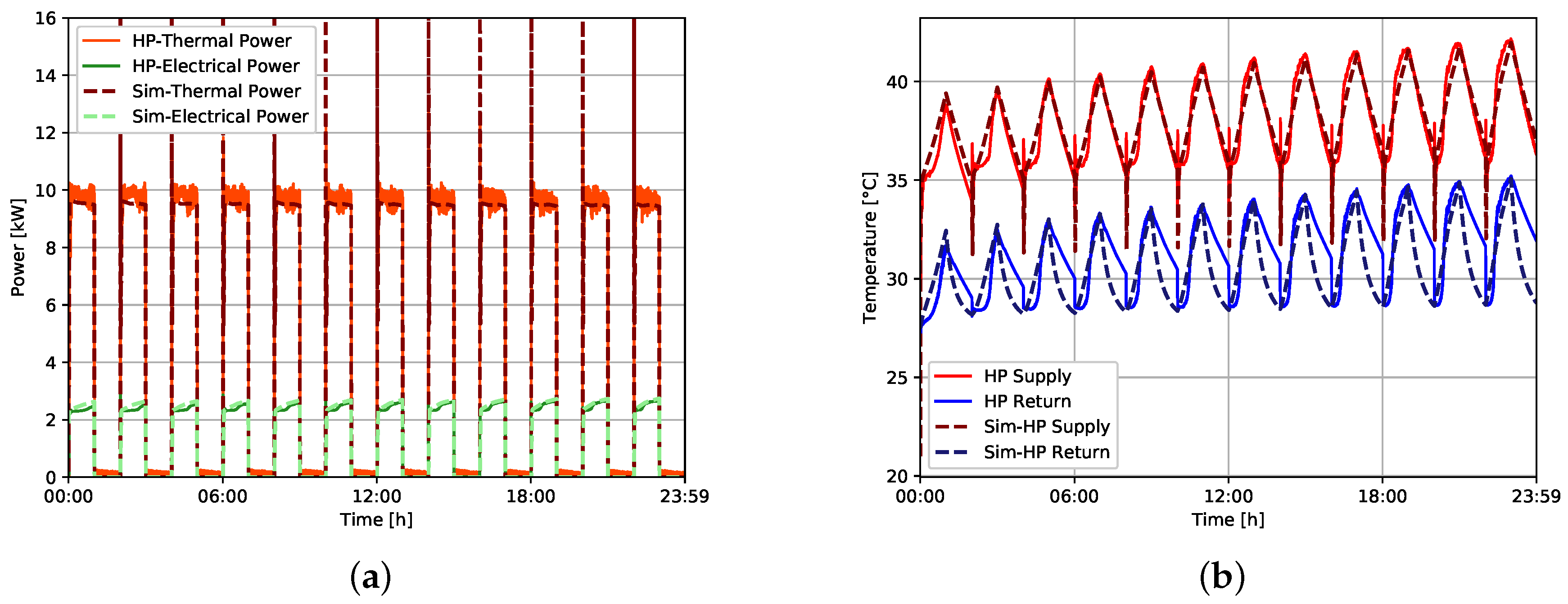
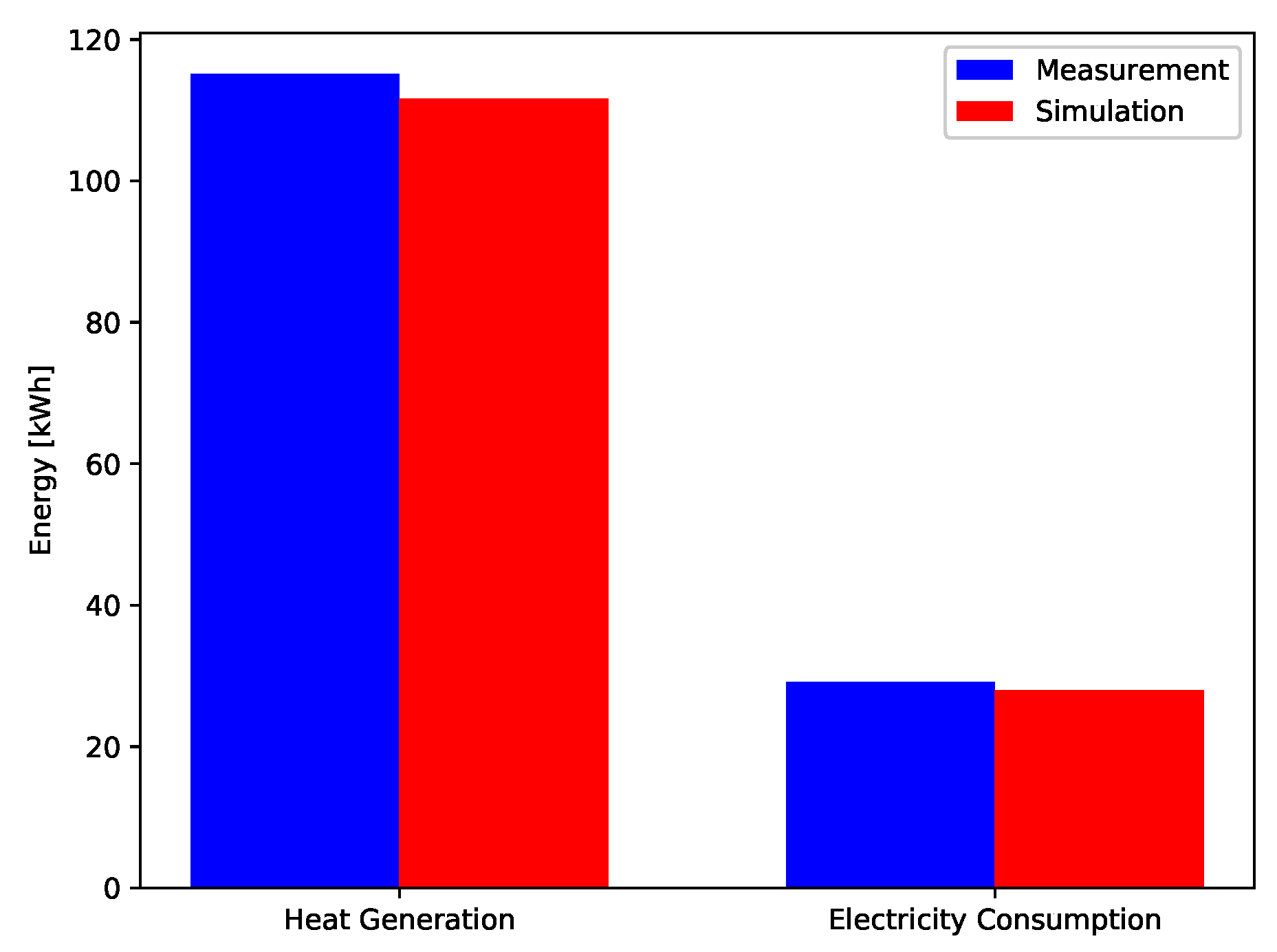
The aforementioned experimental data was used to develop a Modelica model that can accurately model the dynamic behavior of the heat pump. Comparing the daily energy consumption of the measurements of the testbed to the model, it was found that the difference in heat generation and the electricity consumption is only 3% and 4%, respectively. The electrical and thermal power, in addition to supply and return temperatures profiles, were evaluated based on MAPE and RMSD to show the capability of the model to represent the dynamics of the heat pump testbed. The MAPE and RMSD of the temperature profiles reached a value of 1.5% and 0.7 K, respectively.

Moreover, the model can be easily solved for a one-year time horizon of one-second resolution in 22.3 s on a personal computer. Thus, it can be easily integrated into a complete building model without slowing down the solver.

The developed testbed opens the horizon towards several other investigations and demonstration of multiple methods. As a next step, it is planned to integrate the testbed as part of hardware in the loop (HiL) system as presented in [42]. Through that HiL system, a communication can be performed with different models to emulate real-life conditions.

References

1. Bundesministrium für Wirtschaft und Energie. BMWi-Erneuerbare Energien. Available online: https:// www.bmwi.de/Navigation/DE/Themen/themen.html?cl2Categories_LeadKeyword=erneuerbare-energien (accessed on 7 May 2018).
2. Wüstenhagen, R.; Bilharz, M. Green energy market development in Germany: effective public policy and emerging customer demand. Energy Policy 2006, 34, 1681–1696. [Google Scholar] [CrossRef]
3. Bloess, A.; Schill, W.P.; Zerrahn, A. Power-to-heat for renewable energy integration: A review of technologies, modeling approaches, and flexibility potentials. Appl. Energy 2018, 212, 1611–1626. [Google Scholar] [CrossRef]
4. Umwelt Bundesamt. Energieverbrauch für Fossile und Erneuerbare Wärme | Umweltbundesamt. Available online: https://www.umweltbundesamt.de/daten/energie/energieverbrauch-fuer-fossile-erneuerbare-waerme#textpart-1 (accessed on 7 May 2018).
5. Fischer, D.; Madani, H. On heat pumps in smart grids: A review. Renew. Sustain. Energy Rev. 2017, 70, 342–357. [Google Scholar] [CrossRef]
6. Bundesverband Wärmepumpe e.V. Neubau-Statistik 2016: Wärmepumpe Fest Etabliert. Available online: https://www.waermepumpe.de/uploads/media/BWP-Presseinformation_Neubauzahlen_2016.pdf (accessed on 7 May 2018).
7. Li, D.H.; Yang, L.; Lam, J.C. Zero energy buildings and sustainable development implications—A review. Energy 2013, 54, 1–10. [Google Scholar] [CrossRef]
8. Salvalai, G. Implementation and validation of simplified heat pump model in IDA-ICE energy simulation environment. Energy Build. 2012, 49, 132–141. [Google Scholar] [CrossRef]
9. Braun, J.; Bansal, P.; Groll, E. Energy efficiency analysis of air cycle heat pump dryers. Int. J. Refrig. 2002, 25, 954–965. [Google Scholar] [CrossRef]
10. Nekså, P. CO2 heat pump systems. Int. J. Refrig. 2002, 25, 421–427. [Google Scholar] [CrossRef]
11. Wang, X.; Hwang, Y.; Radermacher, R. Two-stage heat pump system with vapor-injected scroll compressor using R410A as a refrigerant. Int. J. Refrig. 2009, 32, 1442–1451. [Google Scholar] [CrossRef]
12. Chua, K.J.; Chou, S.K.; Yang, W.M. Advances in heat pump systems: A review. Appl. Energy 2010, 87, 3611–3624. [Google Scholar] [CrossRef]
13. Haller, M.Y.; Haberl, R.; Mojic, I.; Frank, E. Hydraulic integration and control of heat pump and combi-storage: Same components, big differences. Energy Procedia 2014, 48, 571–580. [Google Scholar] [CrossRef]
14. Miara, M.; Guenther, D.; Kramer, T.; Oltersdorf, T.; Wapler, J. Heat Pump Efficiency—Analysis and Evaluation of Heat Pump Efficiency in Real-Life Conditions; Fraunhofer ISE: Freiburg, Germany, 2011; p. 42. [Google Scholar]
15. Zottl, A.; Nordman, R.; Miara, M.; Number, C. Benchmarking Method of Seasonal Performance. 2012; Available online: http://sepemo.ehpa.org/uploads/media/D4_4_reporting_Benchmarking_method_of_seasonal_performance.pdf (accessed on 7 May 2018).
16. Sayegh, M.; Jadwiszczak, P.; Axcell, B.; Niemierka, E.; Bryś, K.; Jouhara, H. Heat pump placement, connection and operational modes in European district heating. Energy Build. 2018, 166, 122–144. [Google Scholar] [CrossRef]
17. Bastos, H.M.C.; Torres, P.J.G.; Castilla Álvarez, C.E. Numerical simulation and experimental validation of a solar-assisted heat pump system for heating residential water. Int. J. Refrig. 2018, 86, 28–39. [Google Scholar] [CrossRef]
18. Yang, W.; Sun, L.; Chen, Y. Experimental investigations of the performance of a solar-ground source heat pump system operated in heating modes. Energy Build. 2015, 89, 97–111. [Google Scholar] [CrossRef]
19. Liu, F.G.; Tian, Z.Y.; Dong, F.J.; Cao, G.Z.; Zhang, R.; Yan, A.B. Experimental investigation of a gas engine-driven heat pump system for cooling and heating operation. Int. J. Refrig. 2018, 86, 196–202. [Google Scholar] [CrossRef]
20. Harmathy, N.; Murgul, V. Heat Pump System Simulation towards Energy Performance Estimation in Office Buildings. Procedia Eng. 2016, 165, 1845–1852. [Google Scholar] [CrossRef]
21. Zarrella, A.; Emmi, G.; De Carli, M. A simulation-based analysis of variable flow pumping in ground source heat pump systems with different types of borehole heat exchangers: A case study. Energy Convers. Manag. 2017, 131, 135–150. [Google Scholar] [CrossRef]
22. Naldi, C.; Zanchini, E. Dynamic simulation during summer of a reversible multi-function heat pump with condensation-heat recovery. Appl. Therm. Eng. 2017, 116, 126–133. [Google Scholar] [CrossRef]
23. Verhelst, C.; Logist, F.; Van Impe, J.; Helsen, L. Study of the optimal control problem formulation for modulating air-to-water heat pumps connected to a residential floor heating system. Energy Build. 2012, 45, 43–53. [Google Scholar] [CrossRef]
24. Ellerbrok, C. Potentials of demand side management using heat pumps with building mass as a thermal storage. Energy Procedia 2014, 46, 214–219. [Google Scholar] [CrossRef]
25. Nordman, R.; Andersson, K.; Axell, M.; Lindahl, M. Calculation Methods for SPF for Heat Pump Systems For Comparison, System Choice and Dimensioning. SP Rep. 2010, 49, 82. [Google Scholar]
26. Poppi, S.; Sommerfeldt, N.; Bales, C.; Madani, H.; Lundqvist, P. Techno-economic review of solar heat pump systems for residential heating applications. Renew. Sustain. Energy Rev. 2018, 81, 22–32. [Google Scholar] [CrossRef]
27. Ikeda, S.; Choi, W.; Ooka, R. Optimization method for multiple heat source operation including ground source heat pump considering dynamic variation in ground temperature. Appl. Energy 2017, 193, 466–478. [Google Scholar] [CrossRef]
28. Glembin, J.; Büttner, C.; Steinweg, J.; Rockendorf, G. Optimal Connection of Heat Pump and Solar Buffer Storage under Different Boundary Conditions. Energy Procedia 2016, 91, 145–154. [Google Scholar] [CrossRef]
29. Le, K.X.; Shah, N.; Huang, M.J.; Hewitt, N.J. High Temperature Air-Water Heat Pump and Energy Storage: Validation of TRNSYS Models. In Proceedings of the World Congress on Engineering and Computer Science, San Francisco, CA, USA, 25–27 October 2017; Volume II. [Google Scholar]
30. Moreno-Rodríguez, A.; González-Gil, A.; Izquierdo, M.; Garcia-Hernando, N. Theoretical model and experimental validation of a direct-expansion solar assisted heat pump for domestic hot water applications. Energy 2012, 45, 704–715. [Google Scholar] [CrossRef]
31. Ruschenburg, J.; Ćutić, T.; Herkel, S. Validation of a black-box heat pump simulation model by means of field test results from five installations. Energy Build. 2014, 84, 506–515. [Google Scholar] [CrossRef]
32. Domotec, AG. Zirkulationssystem Pipe in Pipe (Rohr in Rohr); Domotec AG: Aarburg, Switzerland, 2018. [Google Scholar]
33. Wehmhörner, U. Multikriterielle Regelung mit Temperaturbasierter Speicherzustandsbestimmung für Mini-KWK-Anlagen. Ph.D Dissertation, München, Germany, 2012. [Google Scholar]
34. TWL-Technologie. Hygiene-Kombispeicher bis 1.000 Liter-TWL-Technologie GmbH. Available online: http://www.twl-technologie.de/de/138098-Hygiene-Kombispeicher-bis-1000-Liter (accessed on 7 May 2018).
35. Mühlbacher, H. Verbrauchsverhalten von Wärmeerzeugern bei dynamisch variierten Lasten und Übertragungskomponenten. Ph.D Dissertation, Technische Universität, München, Germany, 2007. [Google Scholar]
36. Ljubijankic, M.; Nytsch-Geusen, C.; Rädler, J.; Löffler, M. Numerical coupling of Modelica and CFD for building energy supply systems. In Proceedings of the 8th International Modelica Conference, Dresden, Germany, 20–22 March 2011; pp. 286–294. [Google Scholar]
37. Open Modelica System Software. OpenModelica. Available online: https://openmodelica.org/ (accessed on 7 May 2018).
38. ESI ITI. SimulationX 3.8 | Green City. Available online: https://www.simulationx.com/ simulation-software/simulationx3-8.html (accessed on 7 May 2018).
39. El-Baz, W.; Tzscheutschler, P. Autonomous coordination of smart buildings in microgrids based on a double-sided auction. In Proceedings of the 2017 IEEE Power & Energy Society General Meeting, Chicago, IL, USA, 16–20 July 2017; pp. 1–5. [Google Scholar]
40. Glembin, J.; Büttner, C.; Steinweg, J.; Rockendorf, G. Thermal storage tanks in high efficiency heat pump systems—Optimized installation and operation parameters. Energy Procedia 2015, 73, 331–340. [Google Scholar] [CrossRef]
41. Lipp, J.; Sänger, F. Potential of Power Shifting Using a Micro-CHP Units and Heat Storages. In Proceedings of the 3th Internatinal Conference on Microgeneration and related Technologies, Microgen III, Naples, Italy, 4–6 April 2013. [Google Scholar]
42. El-Baz, W.; Sänger, F.; Tzscheutschler, P. Hardware in the Loop ( HIL ) for micro CHP Systems. In Proceedings of the 4th Internatinal Conference on Microgeneration and related Technologies, Microgen IV, Tokyo, Japan, 28–30 October 2015. [Google Scholar]
Figure 1. Simplified hydraulic scheme of the testbed.
Energies 11 01174 g001
Figure 2. The three modules and the heat pump installation in the lab.
Energies 11 01174 g002
Figure 3. Inlet and outlet pipes positions of the storage (left) sensors position across the combi-storage (right). Technical design of the storage [34].
Energies 11 01174 g003
Figure 4. Starting dynamics of the heat pump testbed, (a) heat pump (HP) thermal and electrical power, in addition to the brine thermal power (b) brine supply temperature dynamics because of the mixer circuit.
Energies 11 01174 g004
Figure 5. Control dynamics of module C, (a) supply and return temperature of the space heating circuit (b) the flow rate of the space heating circuit.
Energies 11 01174 g005
Figure 6. The flow of the experimental procedures.
Energies 11 01174 g006
Figure 7. The heat pump model structure.
Energies 11 01174 g007
Figure 8. Performance map of the integrated GSHP (a) COP (b) electrical power (c) thermal power.
Energies 11 01174 g008
Figure 9. Sensor location influence on the number of starts, average COP, and average tank temperature.
Energies 11 01174 g009
Figure 10. Cycling effect on the heat pump system performance, (a) a constant continuous load is maintained throughout the day (b) a constant return temperature is maintained throughout the day.
Energies 11 01174 g010
Figure 11. Modelica heat pump model integrated with the building and storage model of Simulation X.
Energies 11 01174 g011
Figure 12. Temperatures and power dynamics of both the simulation model and the measurements of the testbed, (a) thermal and electrical power (b) supply and return temperatures.
Energies 11 01174 g012
Figure 13. Comparison between the measurements and the simulation model based on the heat generation and the electricity consumption.
Energies 11 01174 g013