Abstract
This study analyzes the short-run hydro generation scheduling for the wind power differences from the contracted schedule. The approach for construction of the joint short-run marginal cost curve for the hydro-wind coordinated generation is proposed and applied on the real example. This joint short-run marginal cost curve is important for its participation in the energy markets and for economic feasibility assessment of such coordination. The approach credibly describes the short-run marginal costs which this coordination bears in “real life”. The approach is based on the duality framework of a convex programming and as a novelty combines the shadow price of risk mitigation, which quantifies the hourly cost of mitigating risk, and the water shadow price, which quantifies the marginal cost of electricity production. The proposed approach is formulated as a stochastic linear program and tested on the case of the Vinodol hydropower system and the wind farm Vrataruša in Croatia. The result of the case study is a family of 24 joint short-run marginal cost curves. The proposed method is expected to be of great interest to investors as it enables risk mitigation for investors with diverse risk preferences, from risk-averse to risk-seeking.
1. Introduction
In this paper the hydro-wind coordination is formulated as a hydro-economic river basin model (HERBM). The coordination assumes that hydro generation is scheduled for firming wind generation. In other words, the short-run hydro generation is scheduled for the wind power differences from the contracted schedule. This wind power difference from contracted schedule impacts the short-run marginal cost (SRMC) curve of the hydro generation curve in the coordination [1]. Generally, a short-run marginal cost curve of a hydro generation is obtained from the water shadow price and as such is important for long-term economic feasibility assessment of the coordination and for short-run competition in electricity markets where these curves are necessary for optimal bidding. In this paper, the joint short-run marginal cost curve for electricity generation of hydro-wind coordinated generation is obtained. To obtain these joint short-run marginal curves, the primal problem and its dual are formulated as convex optimization problems. The primal problem is defined as a short-run revenue maximization problem, while the dual problem minimizes the usage costs of the limited resources (hydro and wind turbine capacity, reservoir capacity, water inflow resource, wind difference resource, risk mitigation capability).
This paper is based on the pioneering works [2,3] which systematically address the problem of the short run profit maximization of the hydro and the pumped storage units using continuous functions and [4] where method for the construction of short-run marginal cost curves for hydro generation is given. These works are based on the ideas of conjugate duality and optimization [5]. The issue of hydro-wind coordination is addressed extensively and among the most significant are the following papers. The sizing method for the pumped hydro storage which uses the wind power surplus is presented in [6]. A methodology for increasing profits of a generation company that owns wind and pumped-storage plants while accounting the wind power uncertainty is presented in [7]. In [8] the problem of introduction of the new pumped-storage station to the existing hydropower system owned by a new subject is addressed. In [9,10] a combined strategy for bidding and operating in a power exchange is presented. It considers the combination of a wind generation company and a hydro-generation company. Related power exchange modeling is discussed in [11,12], a closely related topic of power dispatching in operation and planning is presented in [13,14,15] while power networks control issues are presented in [16]. The [17] discusses the impact of joint bidding of wind power plant and a hydro generating unit on the wind farm revenue in a pool-based electricity market, considering the uncertainty of wind power prediction. The [18] proposes methodology that can reflect different risk profiles of decision makers in wind–hydro-thermal coordination and in [19] a joint operation between a wind farm and a hydro-pump plant is proposed to decrease costs of wind farm imbalances.
This paper will complement these studies by tackling the issue of construction of joint short-run marginal cost curves for the hydro-wind coordination. Obtaining a joint short-run marginal cost curves for a hydro-wind coordination is hard issue due to facts that electricity generation from the hydro-wind coordination is: (a) Storable and; (b) has a negligible direct generation cost. Therefore, usual approach (first derivative by output of the total cost function) for obtainment of short-run marginal cost curves is not sufficient in this case. This issue was not tackled until the fundamental works [4] where issue of constructing short-run marginal cost curve for a hydro producer is analyzed and [1] where the impact of a wind power difference from contracted schedule on the water shadow price is analyzed. This paper, as an extension of the research done in [1,4], contributes with the systematic approach for construction of the joint short-run marginal cost curves for hydro-wind coordination.
Therefore, this research contributes with the approach based on duality method of convex programming for construction of the joint short-run marginal cost curves for electricity generation of a hydro-wind coordination which as a novelty combines: (i) A shadow price of risk mitigation capability, ξ; (ii) and a water shadow price, ψ. The approach enables quantification of hourly cost of risk mitigation through the shadow price of risk mitigation capability, ξ. The proposed approach is formulated as a stochastic linear program and is easy to implement in various optimization problems. The approach is tested on the case study of Vinodol hydropower system and the wind farm Vrataruša in Croatia resulting in a family of 24 joint short-run marginal cost curves. The cost of risk mitigation is also provided. To implement risk mitigation, the conditional value-at-risk (CVaR) risk measure is used, which enables measurement and limitation of extreme financial losses. It is a coherent risk measure [20,21,22,23,24] which means that it satisfies properties of monotonicity, sub-additivity, positive homogeneity and translational invariance. For the risk measure which satisfies these properties it is said that it describes well a real life occurring risks. The properties of sub-additivity and positive homogeneity can be replaced by property of convexity which is important when implementing in convex optimization problems in order not to undermine its convexity (See Corollary 11 in [24] for more about convexity of CVaR.).
Besides the CVaR, the second important term is the water shadow price. The idea behind the water shadow price is that generation of 1 MW∙h in particular hour means not being able to produce that 1 MW∙h in other future hours (it is important to notice that the water shadow price can also be regarded as an opportunity cost of water generation in particular hour). Generally, the shadow price is equal to the marginal utility of relaxing particular constraint or marginal cost when constraint is strengthened. In this case, generation of 1 MW∙h means strengthening water balance constraint by 1 MW∙h, in particular hour. Therefore, by definition, a water shadow price can be regarded as a marginal cost which makes it appropriate for construction of short-run marginal cost curves (For more about issue of shadow pricing of water, see [25] where hydro generation with constant head is analyzed.). In fundamental works [26,27] the water shadow price is assumed to be constant over the planning period [0, T]. For more realistic approach the water shadow price should change over the planning period, such as in [1,2,3,4], every time when reservoir limits are reached, which is also assumed here.
In Section 2, the short-run dual for valuing limited hydro-wind generation resources is set as the double infinite linear programming problem. The dual is reformulated for shadow pricing of water in the coordinated hydro-wind generation. The wind power difference from contracted schedule and CVaR are implemented in the dual problem through the duality framework of convex programming. In the Section 3 cascaded hydropower system Vinodol is carefully modeled as the HERBM [28,29] and the wind farm Vrataruša power difference is implemented within it. The results are presented and discussed in the same Chapter. In the Section 4 conclusions are given.
2. Construction of the Joint Short-Run Marginal Cost Curve
The purpose of the dual optimization problem to the short-run profit maximization is to provide valuations (determine marginal costs/shadow prices) of the hydro-wind resources (reservoir, turbines, water inflows, wind difference, risk mitigation capability). The primal problem is a short-run profit maximization problem shown in Equations (1)–(14). To achieve strong duality, the primal problem must be convex and needs to satisfy Slater’s condition. The primal problem used here is a linear program, i.e., it is convex and it satisfies Linearity constraint qualification which is sufficient condition for strong duality. Strong duality is important here since it implies that the duality gap, i.e., difference between the primal and dual solutions is zero. The dual to the primal problem is shown in Equations (15)–(21) and is used for the construction of the joint short-run marginal cost curves for the hydro-wind coordination.
For hydro generation, it is assumed that minimal and maximal reservoir capacities are and (Equation (6)) and are measured in terms of energy (MW∙h) same as water stock measured which is stored at no cost. The natural water inflow into the reservoir is measured over in MW. Wind power difference is measured over in MW and can obtain positive and negative values (Equation (12)). The units are MW due to continuous-time dating (see Equation (2) and Equation (16)). It is defined as the difference between generated wind power and power indicated in contracted schedule. The hydro turbine operating range in Equation (4) is limited by: its minimal and maximal capacity and measured in MW; the positive and the negative wind difference. The performance curve of the hydro generation is considered linear and the head is fixed over the planning interval . The goal function (Equation (2)) maximizes the expected revenue obtained from day-ahead energy market over the planning interval which is multiplied with the probability of event . The is the hydro generation measured in MW and is the electricity price measured in €/MW∙h since of continuous-time dating. The decision variables in Equation (3), over which the goal function (Equation (2)) is optimized, consist of the electricity generation variable and which are decision variables associated with CVaR risk measure.
According to the Theorem 14 in [24] the CVaR can be implemented in the optimization problem as a goal function, a constraint or both. Since the goal function is predefined here, then CVaR is implemented with Equations (7)–(9). The risk mitigation is done through risk shaping of the special function with the parameter , according to the Theorem 16 in [24]. The is measured in monetary units (€) and represents the minimum desired level of revenue the owner expect in worst outcomes (usually 5%, where ) and is part of input data (Equation (1)). The decision variable in Equation (3) defines the Value at Risk (VaR) measure and is a variable used for determining hourly revenue in worst case events, both these are used for obtainment of the CVaR (For more about CVaR in optimization problems see [19] and Theorems 14 and 16 in [24]). The dual variable of the CVaR constraint Equation (9) is the shadow price (or marginal cost) of risk mitigation capability (risk mitigation capability is considered as a resource). Variable is paired with the r.h.s. of the Equation (9) which is the parameter and the resulting pair is . It is a dimensionless quantity and defines the cost for unit reducing of risk exposure over the planning period . The shadow price of risk mitigation,, in the dual problem (Equation (19)) is linearly dependent on the shadow prices associated with CVaR constraints Equation (7) and Equation (8) and is multiplied by the coefficient . The electricity price is expressed in €/MW∙h. The defines the energy stock at the beginning of planning interval in MW∙h and energy stock surplus or deficit at the end of planning interval in MW∙h. Both parameters are the result of the middle-term HERBM optimization and part of the input data (Equation (1)). The input data is same for primal (Equation (1)), and dual problem (Equation (15)). The in Equation (10) defines the net outflow from the reservoir measured over in MW. When net outflow is integrated over time (Equation (5)) it equals amount of water left at the end of planning horizon, T, which should be above or equal to the predefined level, . Therefore, a primal problem is (the variables denoted after the “;” in equations are the dual variables/shadow prices associated with the constraints):
Given
Maximize
Over
Subject to
where
Its dual:
Given
Minimize
Over
Subject to
where
For hour and for each event , the pairs are obtained, where is the water shadow price and the hydro generation. Each event represents “one dot” in the short-run marginal cost curve for the tth hour as shown in Figure 1d. The Figure 1d is the final short-run marginal cost curve of the hydro-wind coordination. The idea behind the primal and dual problem presented in Equations (1)–(21) is the process of construction which starts with the short-run marginal cost curve of the hydro generation [1,2,3,4] without the impact of wind power difference on the water shadow price [1] as seen on Figure 1a. To include the impact of wind power difference on the water shadow price, the wind power difference , and are implemented as discussed earlier. The resulting curve is one in the Figure 1b where the impact of wind power difference on the water shadow price, , is added to short-run marginal cost of hydro generation. The sign of depends on the sign of the wind power difference i.e., the surplus of wind means which reduces the water shadow price while the shortage of wind means which increases the water shadow price in the coordinated generation [1]. After accounting for the wind differences, the whole short-run marginal cost curve should be horizontally shifted for forecasted wind generation, , as shown in the Figure 1c. This can be done since the effects of the wind generation on the generation range of hydro generation and the availability of water in the reservoir and resulting opportunity costs are already accounted in the previous curve (Figure 1b). Finally, the short-run marginal cost of wind generation should be added in a merit order way (based on ascending order of price). In the Figure 1c the is lower than the water shadow price and is ranked before hydro generation, otherwise it would be ranked last, or somewhere in the middle while shifting right part of the curve.
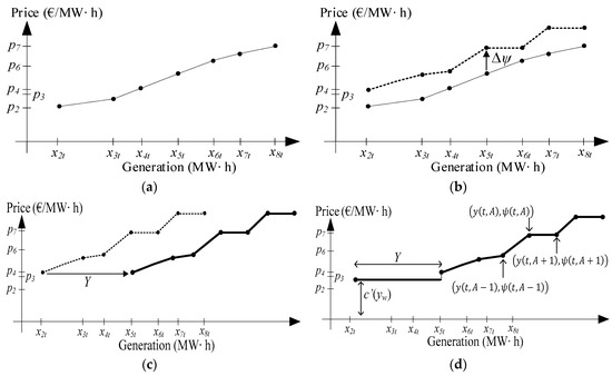
Figure 1.
The example of construction of the joint SRMC curves: (a) hydro generation SRMC; (b) vertical shift due to wind power differences; (c) horizontal shift due to forecasted wind generation; (d) final hydro-wind coordination SRMC.
For the low market price events (and high opportunity cost) this approach would “force” marginal cost curve to adjust itself (horizontally and vertically) until the water shadow price is less or equal than market price for some hour , i.e., . Generally, there is no generation when water shadow price is greater than market price (See Theorem 4.9 in [2].).
The implementation of the presented approach is simple, especially when having in mind that the only needed equation for constructing marginal cost curves is the water shadow price , equation, Equation (21). This equation can be used in the primal problems since the tools for modeling and optimization usually enable readout of the optimal values of the dual variables, i.e., readout of the shadow prices of each constraint. For calculating the water shadow price, the readout of tripe consisting of shadow prices is needed.
3. Case Study and Results
The primal and the dual problems are implemented with the GAMS modeling system under the CPLEX solver (Build 23.9.5, GAMS Software GmbH, Frechen, Germany). The study is done for the 5th December in 2016 on the case of wind farm Vrataruša and hydropower system Vinodol, both located in Croatia. That specific week is considered as the worst-case scenario from the standpoint of water scarcity and wind power differences. It is assumed that wind farm Vrataruša and Vinodol hydropower system (HPS) operate in hydro-wind coordination and that they completely avoid balancing cost. The modeled Vinodol hydropower system consists of: 3 reservoirs, 2 pumped-storage plants (PSP) and 1 hydropower plant (HP), with details given in Table 1 and Figure 2. The energy stock at the beginning/end of a day and the natural water inflows are shown in Table 2. The difference between contracted and actual generated wind power is given in Figure 3. These input parameters are obtained from the real life middle-term operation planning.

Table 1.
HPS Vinodol facilities parameters.
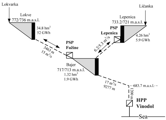
Figure 2.
Model of the Vinodol hydropower system.
Table 2.
Energy stock in percent of maximum reservoir capacity at the beginning of and the end of planning interval.
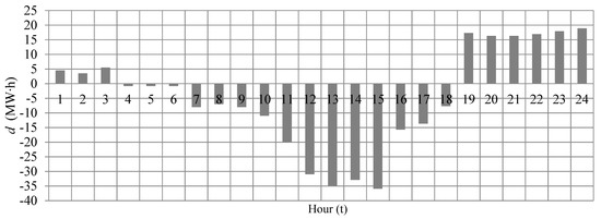
Figure 3.
The wind power difference ( for 5th December of 2016.
The wind farm Vrataruša consists of 14 units, each with 3 MW of installed power. The total installed power is 42 MW with minimum power output 1.1 MW. For the computational effectiveness, only the hydro power plant Vinodol profit is maximized. There is no significant loss in accuracy since the revenue of hydro power plant Vinodol participates with 95% in total system’s revenue. The ramp rate limits of the hydro power plant Vinodol are: MSR (up) 255.15 (MW/min); MSR (down) 340.2 (MW/min). Therefore, there are no constraints on ramping capabilities in the model. The real hydropower system Vinodol has conversion coefficient equal to 5.08 (MW/m3) and is used for frequency regulation ancillary services [29]. A total of 10 electricity price events is generated with the random number generator based on the statistical analyses of the Croatian nodal electricity prices of the first week of December 2016 with the same probability of each event equal to . The CVaR percentile is 85%.
3.1. Results
The results are shown in Table 3, Figure 4 and Figure 5. In Figure 4, the first part of SRMC is vertically shifted upwards due to the increase in the risk mitigation parameter from 0 € to 1380 € for the 16th hour. These phenomena are further explained in the discussion section. The Table 3 shows the dependence of expected daily revenue on the risk mitigation parameter used for hourly risk exposure reduction (it defines the minimum expected return in the 1 − α worst outcomes for each hour). Additionally, Table 3 shows an increase in revenue when the proposed method is applied on hydro-wind coordination due to mitigation of balancing costs compared to uncoordinated business as usual case when wind generation imbalances are penalized (based on yearly average balancing cost prices). The curves in Figure 5 are for the hourly risk exposure of 1380 € and 5 €/ MW∙h of short-run marginal costs of Vrataruša wind farm generation.
Table 3.
Comparison of the expected daily revenue for the coordinated case with proposed method and an uncoordinated case without the proposed method for variations in .
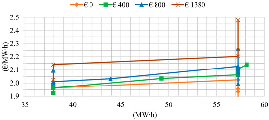
Figure 4.
Part of the 16th hour SRMC curves showing vertical upward shift due to increase in .
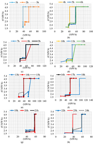
Figure 5.
The SRMC curves for = 1380 € and 5 €/MW∙h electricity generation cost of a Vinodol and Vrataruša hydro-wind coordination from (a) 1st hour to (g) 24th hour for the 5th December in 2016.
3.2. Discussion
Risk mitigation and daily revenue. As parameter used for hourly risk exposure reduction increases from 0 € to 1380 €, the expected daily revenue decreased from 98 885 € to 96 332 € (Table 3).
Risk mitigation and the vertical shift of marginal cost curves. As parameter for hourly risk exposure reduction increases from 0 € to 1380 €, the short-run marginal cost curves (Figure 5) are vertically shifted upwards from 1.9 €/MW∙h to approximately 2.5 €/MW∙h. This means that the hourly risk exposure reduction has a certain cost that can be calculated from the marginal cost curves in Figure 5. In average this cost is 2.5 €/MW∙h–1.9 €/MW∙h = 0.6 €/MW∙h. Therefore 0.6 €/MW∙h is the price of electricity which ensures owner with at least 1380 € in the worst-case scenario. Of course, this insurance is at the expense of the daily revenue, which decreases.
Range of generation in marginal cost curves. The range of generation of Vrataruša-Vinodol coordination is usually from 38 MW∙h to 58 MW∙h (Figure 5). The one general conclusion can be drawn regarding range of generation in joint marginal cost curves, that for low electricity prices (1 h–3 h and 22 h–24 h) there is no desire to produce less than 38 MW∙h. It is obvious that in hours with higher prices (13 h–18 h) coordination want to produce even more than 58 MW∙h and up to 80–90 MW∙h.
Prices in marginal cost curves. The short-run marginal cost curves are characterised by relatively low (compared to market prices) cost which is a result of a low water shadow price. Perfectly inelastic parts of the short-run marginal cost curves are obtained for the values 38 MW∙h and 58 MW∙h (Figure 5).
4. Conclusions
The approach presented in this paper analyses the case of short-run hydro-wind coordination which participates on the electricity market. This research contributes with the approach based on duality method of convex programming for determining the joint short-run marginal cost curves for an electricity generation of the hydro-wind coordination, which as a novelty combines risk mitigation and the water shadow price. The proposed approach is easy to implement in various optimization problems. Proposed method is suitable for investors with various risk preferences, from risk-averse to risk-neutral or risk-seeking, since it enables risk mitigation. It has been shown that the perfectly inelastic short-run marginal cost curves are appropriate for Vrataruša-Vinodol hydro wind coordination which follows from the fact that the water shadow price was constant over the various price events in particular hour. Therefore, it is justified to use simplified method for calculating water shadow price which is constant over the planning period. It has been shown that the risk mitigation has a cost and that this cost is easily quantified which is exemplified and discussed in the paper. In future work, the authors will explore the challenging issues of marginal costs of ancillary services, with emphasis on secondary reserve; as well as improvements to optimal bidding strategies.
Author Contributions
Perica Ilak and Ivan Rajšl have contributed in developing the ideas and formulation of the optimization problem. Josip Đaković and Marko Delimar have been involved in implementation of the problem and analysis of the results. All the authors are involved in preparing the manuscript.
Acknowledgments
This research paper is made possible through the support from Department of Energy and Power Systems of University of Zagreb Faculty of Electrical Engineering and Computing.
Conflicts of Interest
The authors declare no conflict of interest.
Nomenclature
| Symbols | |
| A | An event from the family of all events , . |
| Short-run marginal cost function (€/MW∙h). | |
| Difference between forecasted and actual wind generation (MW). | |
| Positive wind difference (MW). | |
| Negative wind difference (MW). | |
| Natural water inflow (MW). | |
| Special function used for risk shaping of CVaR (€). | |
| Sigma algebra which defines all possible events in hour . | |
| Net outflow of hydro generation (MW) | |
| Hourly revenue (€). | |
| Maximal capacity of reservoir (MW∙h). | |
| Parameter used for risk exposure reduction in risk shaping procedure (€). | |
| Hydro turbine maximal capacity (MW). | |
| Wind turbine maximal capacity (MW). | |
| Minimal capacity of reservoir (MW∙h). | |
| Hydro turbine minimal capacity (MW). | |
| Wind turbine minimal capacity (MW). | |
| Probability of the event and consequently probability of realization of the price | |
| Energy stock, amount of water in reservoir in t, (MW∙h). | |
| Energy stock at the beginning of planning interval (MW∙h) | |
| Energy stock surplus or deficit at the end of planning interval (MWh) | |
| Hydro generation (MW). | |
| Y | Contracted wind generation (MW). |
| Actual wind generation (MW). | |
| Greek | |
| Percentile used for the CVaR where 1- defines the worst events (%). | |
| Shadow prices associated with constraint of CVaR’s helping variable (€). | |
| Shadow prices associated with CVaR’s hourly revenue constraint. | |
| The decision variable which defines the Value at Risk (€). | |
| Variable used for obtainment of the CVaR (€). | |
| Shadow price of hydro generation maximum capacity (€/MW∙h). | |
| Shadow price of reservoir maximum capacity (€/MW∙h). | |
| Shadow price of energy stock surplus/deficit at the end of operation(€/MW∙h). | |
| Shadow price of hydro generation minimum capacity (€/MW∙h). | |
| Shadow price of reservoir minimum capacity (€/MW∙h). | |
| Shadow price of risk mitigation capability (dimensionless). | |
| Price of electricity (€/MW∙h). | |
| Shadow price of water (€/MW∙h). | |
| Spaces | |
| Planning interval, subspace of the real line . | |
References
- Ilak, P.; Rajšl, I.; Krajcar, S.; Delimar, M. The impact of a wind variable generation on the hydro generation water. Appl. Energy 2015, 154, 197–208. [Google Scholar] [CrossRef]
- Horsley, A.; Wrobel, A.J. Efficiency Rents of Storage Plants in Peak-Load Pricing, II: Hydroelectricty; London School of Economics & Political Science (LSE): London, UK, 1999. [Google Scholar]
- Horsley, A.; Wrobel, A.J. Efficiency Rents of Storage Plants in Peak-Load Pricing, I: Pumped Storage; London School of Economics & Political Science (LSE): London, UK, 1996. [Google Scholar]
- Ilak, P.; Krajcar, S.; Rajšl, I.; Delimar, M. Pricing Energy and Ancillary Services in a Day-Ahead Market for a Price-Taker Hydro Generating Company Using a Risk-Constrained Approach. Energies 2014, 7, 2317–2342. [Google Scholar] [CrossRef]
- Rockafellar, R.T. Conjugate Duality and Optimization; Siam: Philadelphia, PA, USA, 1974. [Google Scholar]
- Kaldellis, J.K.; Kapsali, M.; Kavadis, K.A. Energy balance analysis of wind-based pumped hydro storage systems in remote island electrical networks. Appl. Energy 2010, 87, 2427–2437. [Google Scholar] [CrossRef]
- Varkani, A.K.; Daraeepour, A.; Monsef, H.A. A new self-scheduling strategy for integrated operation of wind and pumped-storage power plants in power markets. Appl. Energy 2011, 88, 5002–5012. [Google Scholar] [CrossRef]
- Rajšl, I.; Ilak, P.; Delimar, M.; Krajcar, S. Dispatch Method for Independently Owned Hydropower Plants in the Same River Flow. Energies 2012, 5, 3674–3690. [Google Scholar] [CrossRef]
- Angarita, J.M.; Usaola, J.G. Combining hydro-generation and wind energy: Biddings and operation on electricity spot markets. Electr. Power Syst. Res. 2007, 77, 393–400. [Google Scholar] [CrossRef]
- Angarita, J.L.; Usaola, J.; Martínez-Crespo, J. Combined hydro-wind generation bids in a pool-based electricity market. Electr. Power Syst. Res. 2009, 79, 1038–1046. [Google Scholar] [CrossRef]
- Bahrami, S.; Amini, M.H. A decentralized trading algorithm for an electricity market with generation uncertainty. Appl. Energy 2018, 218, 520–532. [Google Scholar] [CrossRef]
- Bahrami, S.; Toulabi, M.; Ranjbar, S.; Moeini-Aghtaie, M.; Ranjbar, A.M. A Decentralized Energy Management Framework for Energy Hubs in Dynamic Pricing Markets. IEEE Trans. Smart Grid 2017. [Google Scholar] [CrossRef]
- Samadi, P.; Bahrami, S.; Wong, V.W.S.; Schober, R. Power dispatch and load control with generation uncertainty. In Proceedings of the 2015 IEEE Global Conference on Signal and Information Processing (GlobalSIP), Orlando, FL, USA, 14–16 December 2015; pp. 1126–1130. [Google Scholar]
- Mohammadi, A.; Mehrtash, M.; Kargarian, A. Diagonal Quadratic Approximation for Decentralized Collaborative TSO+DSO Optimal Power Flow. IEEE Trans. Smart Grid 2018. [Google Scholar] [CrossRef]
- Elsaiah, S.; Cai, N.; Benidris, M.; Mitra, J. Fast economic power dispatch method for power system planning studies. IET Gener. Transm. Distrib. 2015, 9, 417–426. [Google Scholar] [CrossRef]
- Boroojeni, K.G.; Amini, M.H.; Nejadpak, A.; Iyengar, S.S.; Hoseinzadeh, B.; Bak, C.L. A theoretical bilevel control scheme for power networks with large-scale penetration of distributed renewable resources. In Proceedings of the 2016 IEEE International Conference on Electro Information Technology (EIT), Grand Forks, ND, USA, 19–21 May 2016; pp. 0510–0515. [Google Scholar]
- Vieira, B.; Viana, A.; Matos, M.; Pedro, J. A multiple criteria utility-based approach for unit commitment with wind power and pumped storage hydro. Electr. Power Syst. Res. 2016, 131, 244–254. [Google Scholar] [CrossRef]
- Duque, J.; Castronuovo, E.D.; Sánchez, I.; Usaola, J. Optimal operation of a pumped-storage hydro plant that compensates the imbalances of a wind power producer. Electr. Power Syst. Res. 2011, 81, 1767–1777. [Google Scholar] [CrossRef]
- Rockafellar, R.T.; Uryasev, S. Optimization of conditional value-at-risk. J. Risk 1998, 2, 21–41. [Google Scholar] [CrossRef]
- Artzner, P.; Delbaen, F.; Eber, J.M.; Heath, D. Thinking coherently. Risk 1997, 10, 68–91. [Google Scholar]
- Acerbi, C. Spectral measures of risk: A coherent representation of subjective risk aversion. J. Bank. Financ. 2002, 26, 1505–1518. [Google Scholar] [CrossRef]
- Follmer, H.; Schied, A. Convex and Coherent Risk Measures; Humboldt University: Berlin, Germany, 2008. [Google Scholar]
- Rockafellar, R.T. Coherent Approaches to Risk in Optimization Under Uncertanty. Tutor. Oper. Res. Inf. 2007, 3, 38–61. [Google Scholar]
- Rockafellar, R.T.; Uryasev, S. Conditional Value-at-Risk for General Loss Distributions. J. Bank. Financ. 2002, 26, 1443–1471. [Google Scholar] [CrossRef]
- Perekhodtsev, D.; Lave, L. Efficient Bidding for Hydro Power Plants in Markets for Energy and Ancillary Services; MIT Center for Energy and Environmental Policy Research: Cambridge, MA, USA, 2005. [Google Scholar]
- Koopmans, T.C. Water Storage Policy in a Simplified Hydroelectric System. In Proceedings of the First International Conference on Operational Research, Oxford, UK, 2–5 September 1957. [Google Scholar]
- Warford, J.; Munasinghe, M. Electricity Pricing: Theory and Case Studies; International Bank for Reconstruction and Development: Baltimore, MD, USA; London, UK, 1982. [Google Scholar]
- Zhang, H.; Gao, F.; Wu, J.; Liu, K.; Liu, X. Optimal Bidding Strategies for Wind Power Producers in the Day-ahead Electricity Market. Energies 2012, 5, 4804–4823. [Google Scholar] [CrossRef]
- Ilak, P.; Krajcar, S.; Rajšl, I.; Delimar, M. Profit Maximization of a Hydro Producer in a Day-Ahead Energy Market and Ancillary Service Markets. In Proceedings of the IEEE Region 8 Conference EuroCon, Zagreb, Croatia, 1–4 July 2013. [Google Scholar]
© 2018 by the authors. Licensee MDPI, Basel, Switzerland. This article is an open access article distributed under the terms and conditions of the Creative Commons Attribution (CC BY) license (http://creativecommons.org/licenses/by/4.0/).