Dynamic Programming-Based Vessel Speed Adjustment for Energy Saving and Emission Reduction

Abstract

Maritime transportation is an economic form of mass transportation, but it is associated with significant energy consumption and pollutant emissions. External forces such as tidal currents, waves, and wind strongly influence the energy efficiency of ships. The effective management of external forces can save energy and reduce emissions. This study presents a method to build an optimal speed adjustment plan for a ship to navigate a given route. The method takes a dynamic programming (DP)-based approach to finding such an optimal plan to utilize external forces. To estimate the speed changes caused by external forces, the proposed method uses the mapping information from a combined database of ship status, marine environmental conditions, and speed changes. For the efficient manipulation of externally forced speed-change information, we used MapReduce-based operations that can handle big data and support the easy retrieval of associated data in specific situations. To evaluate the applicability of the proposed method, we applied it to real navigation situations in the southwestern sea of the Korean Peninsula. In the simulation experiments, we used real automatic identification system data and marine environmental data. The proposed method built more efficient speed adjustment plans than the fixed-speed navigation in terms of energy savings and pollutant emission reduction. The results also showed that the speed adjustment exploits external forces in a beneficial manner.

1. Introduction

Maritime transportation has played an important role in international goods transportation. Large ships have a massive load capacity and consume large amounts of fossil fuels to operate [1]. High energy consumption entails high pollutant emissions that have adverse impacts on the marine and atmospheric environment and on public health [2]. Hence, in this study, we are concerned with the efficient navigation of ships to save energy and reduce pollutant emissions.

Liner ships and passenger ships commute similar routes because of safety and regulations [3]. Therefore, a route change or an adjustment is not an option to save energy and reduce emissions, which makes speed adjustment on navigation routes necessary. Marine environmental conditions such as tidal currents, waves, and wind greatly affect navigation speeds, as external forces either in a friendly or an aggressive manner assist or block a ship’s navigation. Hence, speed should be adjusted to exploit friendly external forces and moderate the effects of aggressive forces.

External forces change a ship’s speed, which depends on the ship’s characteristics and geographic position. To incorporate the effects of external forces into speed adjustment, it is necessary to have the mapping information regarding the ships’ characteristics, geographical position, and marine environmental conditions [4]. In this paper, we present a method to extract such mapping information from the ships’ automatic identification system (AIS) data and the marine environmental data. To determine an optimal speed adjustment plan, we propose a dynamic programming (DP)-based method that examines all possible adjustment plans under imposed constraints. As the performance criteria, we use the total energy consumption along with the amount of pollutant emissions. The proposed DP-based method can determine an optimal speed-change plan for voyages for which there are sufficient AIS and marine environmental data.

The remainder of the paper is organized as follows: Section 2 presents the related work for route optimization, and Section 3 presents a MapReduce-based processing method to estimate the externally forced speed changes. Section 4 presents how to estimate the energy consumption and the quantity of pollutant emissions. Section 5 proposes a DP-based method to identify optimal speed adjustment plans for a given navigation route. Section 6 gives the experimental results to evaluate the effectiveness of the proposed method, and Section 7 presents the conclusions.

2. Related Work

The representative data related to vessel route optimization are the AIS data and the marine environmental data. AIS data consist of a ship’s ID, position, course, heading, speed, time, and more. Ships broadcast their AIS messages on a regular basis (every 2–10 s) so that the shore-side monitoring stations and neighboring ships can receive the messages [5]. When the AIS data are combined with the ship’s registry and logistics data, the ship’s detailed specifications and loading status can be retrieved. The marine environmental data contain the velocity (i.e., direction and speed) of tidal currents, waves, wind, and other measurements, such as temperature. These are measured at the sensor buoys installed offshore. The number of such buoys is limited, but they are important sources of data acquisition to provide key information on external forces.

There has been some previous work on efficient navigation with optimal routes. Hanssen and James proposed the isochrone method to determine an optimal route, which has been long used owing to its easy computation [6]. Hagiwa proposed an enhanced version of the isochrone method for efficient route computation [7]. Jung and Rhyu proposed a heuristic algorithm based on the A* algorithm to determine an economical shipping route [8]. Zhang and Huang proposed a method to determine an optimal route according to weather changes [9]. Choi et al. proposed an eight-point Dijkstra algorithm based method to determine an economical shipping route by estimating the fuel consumption with the ship’s speed reduction on the basis of the ship’s voyages and weather forecast data [10]. All these methods attempt to find new routes to optimize given criteria such as safety and energy consumption. Our interest is not in finding new routes, but to adjust the speed of ships on a given route in situations for which route changes may cause new problems such as safety concerns and regulation violations.

Wang et al. proposed a ship speed adjustment method that uses a wavelet neural network model for predicting the next state of the wind speed and water depth with their six consecutive preceding states and that determines an optimal speed on the basis of the predicted state [11]. Their method was developed for river navigation, for which conditions do not severely change compared to the open sea. It does not consider the navigation time constraint, and hence their energy-efficient speed adjustment plan may fail to enable the ship to arrive at a destination in time. Du et al. proposed a mixed-integer linear programming model to solve the berthing allocation problem; it determines a speed adjustment plan with consideration of the tide height and required time of arrival [12]. Oil Companies International Marine Forum proposed the “virtual arrival policy”, which adjusts the sailing speed in order to update ship arrival times when there are known delays caused by berth availability at the destination port [13]. The above-mentioned methods do not consider the externally forced speed changes in their speed adjustment plans. Dulebenets et al. proposed a hybrid evolutionary-algorithm-based method for solving the berth scheduling problem, which minimizes the total service cost, including the carbon dioxide emission cost at a marine container terminal [14]. Their method concerns only the terminal operations and does not consider the speed adjustment plan in the open sea.

Energy consumption and pollutant emissions are of concern in optimal speed adjustment during navigation. Energy consumption is affected by various factors such as the engine, ship type and shape, and loading state. Some methods have been developed to approximately estimate energy consumption by ships. Browning and Bailey proposed a model that estimates energy consumption in terms of maximum engine power, load factor, and activity hours [15]. The amount of pollutant emissions is usually assumed to be proportional to the energy consumption. Several emission estimation models have also been proposed. These can be categorized into top-down and bottom-up methods. Top-down methods allocate the total fuel consumption to individual ships, shipping routes, or shipping areas using statistical analysis methods [16]. Bottom-up methods gather information about individual ship activities and sum this up to obtain the energy consumption.

3. MapReduce-Based Estimation of Externally Forced Speed Changes for Oceangoing Ships

The speed and course of ships are affected by environmental factors such as tidal currents, waves, and wind. Tidal currents and waves are particularly important for ship passage plans, such as for estimating the time of arrival and ship’s routes [17]. Therefore, maritime security agencies have developed numerical models based on the environmental sensor data for tidal currents and waves and use these for maritime safety and rescue services [18]. The external force estimation models are numerical models developed from the sensor data of external forces or data generated by marine environment models for tidal currents and waves [19]. The effect of external forces on external force estimation models is important and is strongly dependent on the structure, type, and freight loading state of a ship. In this section, we present a method to compute the external forces acting on a ship that is based on a ship’s AIS data and marine environment sensor data. The MapReduce-based processing method can handle the big data produced by a ship’s AIS and marine environmental monitoring stations and estimates external forces (Figure 1).

3.1. Identification of Reference Ships and Associated Information

The information on reference ships and their speed over water (SOW) is used to compute the externally forced speed changes, where the SOW is assumed to have no external disturbances. The changes in the externally forced speed due to marine environmental factors are estimated by the difference between the SOW and the effective speed, called the speed over ground (SOG) [20]. The ship’s SOW data are measured by the Doppler speed log sensor installed at the bottom of the vessel. The SOW data are not loaded into the AIS signal and are not usually delivered to the shore-side monitoring stations or other ships. This means that the SOG data are extracted from the AIS data, but the SOW data are only estimated. The method is employed to estimate the SOW data, where the speeds over the sea are used with the marginal effect of conditions of tidal currents, waves, and wind. Further, the mean and standard deviation of the speed are computed according to the vessel ID and cargo status. On the basis of the computations, reference vessels are selected according to the small standard deviations, also referred to as reference ships. The speeds of the reference ships are assembled in a database along with the information on their length, cargo loading status, and reference speed (

Table 1. Example of reference ship database.

Ship ID	Length	Cargo Status	Reference Speed
1	174	Unloaded	15.970
2	133	Unloaded	13.032
3	132	Loaded	12.118
4	113	Loaded	12.573
5	143	Passenger ship	17.466
:	:	:	:
:	:	:	:

). This information is later used to estimate the SOW for new vessels traveling over the region. The most similar reference ship to a new vessel is determined on the basis of the ship type, length, and cargo loading status. We use the speed of the most similar reference ship for the SOW of the new vessel.

3.2. Estimation of Externally Forced Speed Changes

We need an efficient method to process marine environmental data and AIS data for extracting important statistical information. We propose the MapReduce-based method, which parallelizes the data processing tasks with the map and reduce operations. The map operations extract information from raw data as key-value pairs, where the key is the identifier and the value is the associated value of a specific attribute. The reduce operations aggregate the values with the same key in the number of key-value pairs. The MapReduce-based method is efficiently executed in a distributed computing environment such as Hadoop [21], which is an open-source platform for big data processing on a large number of commodity computers.

To estimate the externally forced speed changes, we collect the speed-change data based on the ship characteristics and marine environmental factors. Such characteristics and factors contain some continuous attribute values, which makes it difficult to use the MapReduce-based parallel processing. Hence, we discretize their domain into a finite number of partitions. We call the partitioned representation of ship characteristics the “ship index” and the partitioned marine environmental factors the “marine environment index”.

AIS data contain both static and dynamic information of a ship [22]. The static information consists of the ship’s identifiers, such as the call sign, length, tonnage, fore and aft draft, destination port of the current voyage, and freight loading status. The dynamic information contains the speed, course, and the location of the ship. Almost every ship, except for small fishing boats, broadcasts its AIS data nearly every 2–10 s. The shore-side maritime monitoring authorities transfer these AIS data into their own databases. For MapReduce processing, important ship characteristics are encoded in the ship index (

Table 2. Ship indices and their associated attribute values.

Ship Index	Ship Type	Length (m)	Tonnage (K/T)	Height (m)	Depth (m)	Location (Geohash)	Course (Direction)	Speed (kt)
1	Cargo	0–75	0–1	0–5	2–4	wvcy	N	10
2	Cargo	0–75	0–1	5–10	2–4	wvcz	NE	11
3	Cargo	75–150	7–8	5–10	6–8	wvfn	E	12
4	Container	75–150	8–9	0–5	6–8	wy1b	SE	13
5	Container	75–150	9–10	5–10	8–10	wy1c	E	14
:	:	:	:	:	:	:	:	:

), which is assigned a combination of eight discretized attributes: the ship type, length, tonnage, height, draft mark, position, course, and speed. The ship type attribute is one of the following seven categories: general cargo ship, dangerous goods carrier, container, car carrier, passenger ship, towing vessel, or miscellaneous vessels. The value domain of the length attribute is partitioned into equal lengths of 75 m, for example, (0, 75], (75, 150], (150, 225], and so on. The value domain of the tonnage attribute is partitioned into equal weights of 1 kiloton(K/T): (0, 1], (1, 2], (2, 3], and so on. The value domains of the height and draft marks are partitioned into equal intervals of 5 and 2 m, respectively. The location in longitude and latitude is represented using Geohash level 4, where Geohash is a geocoding system that encodes a geographic location into a short string of letters and digits. Geohash level 4 has a code for each block with an approximate size of 39.4 km × 19.5 km [23]. The course attribute has a value from eight directions: E, NE, W, SW, S, SE, N, and NW. The value domain of the speed attribute is partitioned into equal intervals of 1 knot (kt) starting from 10 kt. A ship index is assigned to a combination of these attribute values, whose occurrence is larger than the specified threshold hold.

The ship speed and course are affected by tidal currents, waves, and wind. These factors have both direction and magnitude components. The possible combinations of these environmental factors are partitioned into a finite number of groups. We use eight directional symbols with respect to the course direction. The speed of tidal currents is represented by 0.5 kt unit intervals, wave height is represented by 1 m unit intervals, and wind speed is represented by 5 kt intervals. A marine environmental index is assigned to a combination of environmental factors (

Table 3. Example of marine environment index.

Marine Environment Index	Current (Direction, kt)	Wave (Direction, m)	Wind (Direction, kt)
1	N, 0–0.5	N, 0–1	N, 0–5
2	N, 0–0.5	N, 1–2	NE, 0–5
3	N, 0–0.5	N, 2–3	NE, 5–10
4	N, 0–0.5	N, 3–4	NE, 10–15
5	N, 0–0.5	NE, 0–1	NE, 15–20
6	N, 0–0.5	NE, 1–2	E, 0–5
57	N, 0–0.5	NE, 2–3	E, 5–10
:	:	:	:

).

To estimate the externally forced speed changes for various locations and environmental conditions, the following MapReduce tasks are carried out: The map and reduce functions take and return key-value pairs [24]. From the reference ship database, the reference ship and the reference speed corresponding to the course of the vessel are retrieved. The difference between the reference speed and the current speed of the ship is the externally forced speed change at the position of the ship, which is stored in the externally forced speed-change database. The externally forced speed-change database is organized as a key-value store, where the key is the ship index and marine environmental index, and the value is the speed change caused by external forces.

Figure 2 shows the MapReduce operations to produce pairs of the keys (ship index and marine environmental index) and their associated speed-change value. The mapper generates keys and their value by retrieving the relevant records from the AIS and marine environmental databases and encodes them using the discretizing indexing methods. The input data consist of the marine environmental index, ship index, and speed change. The two indexes are combined into a character string key, and their associated speed change is treated as its value to the key. The reducer aggregates values with the same key to a single quantity. For instance, in the reducing phase of Figure 2, when the reducer receives the key “12_4” and its associated speed changes [1; 1.1; 0.8; 0.8; 0.9; 1.1; …], it sends out the pair of the key “12_4” and the average value 0.95 of the speed changes. The mapper and reducer are parallelized and distributed; hence, the MapReduce processing method can handle a large volume of AIS and marine environmental data.

4. Energy Consumption and Emission Quantity Estimation

We aim to find an optimal speed adjustment plan for a route that minimizes the emissions and energy consumption. There are some numerical models for estimating energy consumption and emissions [15]. Energy consumption for a vessel navigation is modeled as a function of the maximum continuous rating power $P_{mcr}$ of the engine, load factor $LF$, and activity A, as follows:

$$\mathrm{C}=P_{mcr}\times A\times LF,$$

(1)

where $P_{mcr}$ is the maximum engine power (kW) of the ship, which is a unique characteristic of a ship; $A$ is the operating hours of the ship (h); and $LF$ is the load factor, which is expressed as a percentage of the ship’s total power. At the service or cruise speed, the load factor is 83%. At lower speeds, the propeller law is used to estimate the load factor as follows:

$$LF={\left(\frac{V_{SOG}}{V_{max}}\right)}^3,$$

(2)

where $V_{SOG}$ is the speed over ground (kt), and $V_{max}$ is the maximum speed (kt), which is 1.064 times Lloyd’s service speed.

The amount of emissions from an engine is proportional to the energy consumption. Emissions can be estimated using the following numerical model:

$$E=C\times EF\times FCF,$$

(3)

where $E$ is the amount of pollutant emissions (g), $C$ is the energy consumption (kWh) computed using Equation (3), $EF$ is the emissions factor (g/kWh), and $FCF$ is the fuel correction factor.

Figure 3 shows the components of emission calculations and the sources of information. The information for $P_{mcr}$ was collected from the Korean Register of Shipping [25], a classification society to verify and certify the services for ships and marine structures in Korea, and from the Port Management Information System (PORT-MIS) [26], a port logistics information system to manage the entry and departure of ships, using facilities within ports, port traffic control, cargo entering and carrying, and tax collection in Korean trade ports. The load factor $LF$ is computed using Equation (2) with the SOG and SOW estimated using the MapReduce-based operations presented in Section 3. The load factor for the voyage of a ship is determined using the AIS data for the ship, marine environmental data, externally forced speed-change data, and reference ship data.

The emissions of pollutants such as particulate matter (PM), nitrogen oxides (NO_x), carbon oxides (CO_x), sulfur oxides (SO_x), hydrocarbons (HC), methane (CH₄), and nitrous oxide (${\mathrm{N}}_2\mathrm{O}$) are computed using Equation (3). The emission factors $EF$ are reported in previous studies [27]. Residual oil is used to operate the vessel’s main engine and is considered an intermediate fuel with an average sulfur content of 2.7%. The emission factors using residual oil in oceangoing ships are shown in

Table 4. Emission factors for oceangoing ships (g/kWh) [15].

Engine	PM	$\mathbf{N}{\mathbf{O}}_{\mathbf{x}}$	$\mathbf{S}{\mathbf{O}}_{\mathbf{x}}$	CO	HC	$\mathbf{C}{\mathbf{O}}_2$	$\mathbf{C}{\mathbf{H}}_4$	${\mathbf{N}}_2\mathbf{O}$
Diesel	1.2	13.0	11.5	1.1	0.5	683	0.010	0.031

[15].

The emission rates are adjusted by the correction factors for engines and residual fuel with 1.5% sulfur content (

Table 5. Fuel correction factors [28].

Fuel	PM	$\mathbf{N}{\mathbf{O}}_{\mathbf{x}}$	$\mathbf{S}{\mathbf{O}}_{\mathbf{x}}$	CO	HC	$\mathbf{C}{\mathbf{O}}_2$	$\mathbf{C}{\mathbf{H}}_4$	${\mathbf{N}}_2\mathbf{O}$
Heavy Fuel Oil	0.82	1.00	0.56	1.00	1.00	1.00	1.00	1.00

) [28].

5. The Proposed Optimal Navigation Search Method for Emission and Energy

Emissions and energy consumption during the navigation of an oceangoing vessel depend on the vessel’s speed. The navigation route for a voyage is prespecified on the basis of the regulations and environmental conditions. The speed of an oceangoing vessel is affected by external forces such as tidal currents, waves, and wind. Tidal currents show some patterns according to the lunar calendar time and date, and wind shows seasonal patterns. Section 3 shows how to extract the patterns of externally forced speed changes for days of the year in regions from big marine environmental data. The effective speed of a navigating vessel is computed by combining the SOW and the externally forced speed change. The effective speed allows us to compute the real emissions and energy use over the voyage. The vessels usually navigate an ocean route at a fixed speed; it is, however, possible to save emissions and energy by adjusting the speed. An optimal speed adjustment plan should be computed by considering the SOW, externally forced speed changes, and the arrival time.

Here, we propose a DP-based method that efficiently computes an optimal speed adjustment plan along with total emissions. DP is a means for solving a complex problem by breaking it into smaller subproblems, solving each of them once and storing their solutions, and using them to construct the solution to the original problem [29].

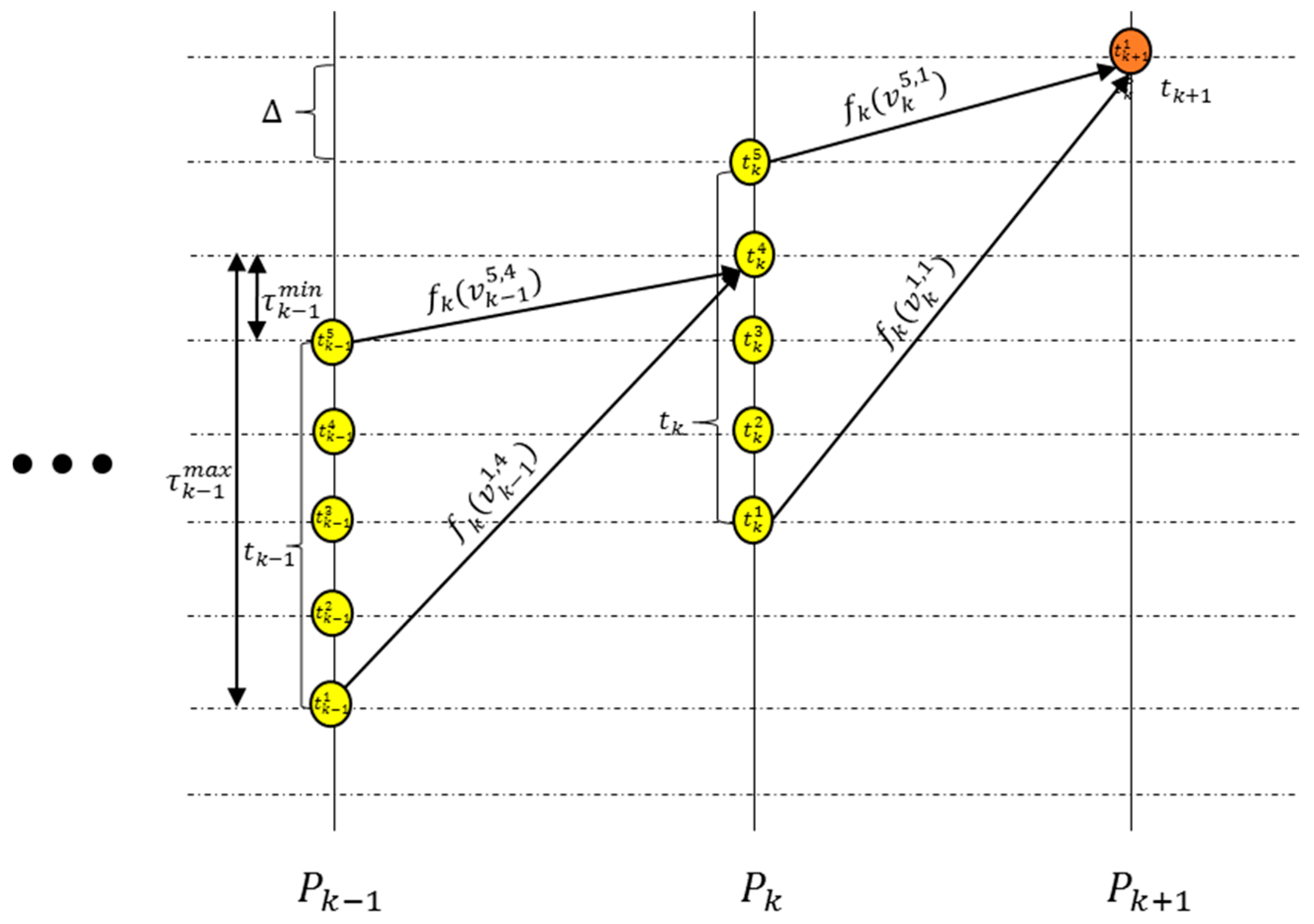
In DP, we use the following settings and notations: A navigation route $R$ is expressed in a sequence of positions, $R=(P_1,P_2,\dots ,P_N)$, where $P_k$ is the location of index $k$ and N is the number of position indices; $t_k$ indicates the time at which a vessel is at position $P_k$, and it has a value from the set $t_k^1$, $t_k^2$, …, $t_k^{u_k^i}$; $t_k^1$ is the earliest time at which the vessel arrives at location $P_k$ starting from time $t_{k-1}^1$, and $t_k^i=t_k^1+\Delta (i-1)$, where $\Delta$ is the time interval of considered arrival times at each position; ${\tau }_{k-1}^{min}$ indicates the minimum time taken for the vessel to travel from $P_{k-1}$ to $P_k$ with the fastest speed allowed [30]. Therefore, the following relationship holds:

$$t_k^1=t_{k-1}^1+{\tau }_{k-1}^{min}, i=1, \dots , u_k^i.$$

(4)

In Equation (4), $u_k^i$ denotes the index of the most recent time at which the vessel can depart from $P_{k-1}$ to reach $P_k$ within the considered time, that is, $u_k^i=\max \{l|t_{k-1}^l\le t_k^i+{\tau }_{k-1}^{max}\},$ where ${\tau }_{k-1}^{max}$ is the minimum time taken for the vessel to travel from $P_{k-1}$ to $P_k$; $e_k^{t_k^i}$ denotes the externally forced speed at time $t_k^i$ at position $P_k;$ $f_{k-1}(v_{k-1}^{j,i})$ indicates the energy consumption to travel from $P_{k-1}$ to $P_k$ with SOW $v_{k-1}^{j,i}$ and externally forced speed $e_{k-1}^{t_{k-1}^i}$; and $T_k(v_k,e_k^{t_k^i})$ is the time for the vessel to travel from $P_{k-1}$ to $P_k$ with speed $v_k$ and externally forced speed $e_k^{t_k^i}$ at time $t_k^i$. Therefore, ${\tau }_{k-1}^{min}$ is computed as follows:

$${\tau }_{k-1}^{min}=T_{k-1}(V_{max},e_{k-1}^{t_{k-1}^1}).$$

(5)

The accumulated energy consumption (Figure 4) for a vessel to arrive at position $P_k$ at time $t_k^i$ can be recursively calculated as follows:

$$\mathrm{C}\left(P_k,t_k^i\right)=mi{n}_j\left\{C\left(P_{k-1},t_{k-1}^j\right)+f_{k-1}(v_{k-1}^{j,i})\right\}$$

(6)

$$1\le j\le u_k^i, \mathrm{where} u_k^i=\max \{l|t_{k-1}^l\le t_k^i+{\tau }_{k-1}^{min}\}$$

To determine an optimal speed adjustment plan, the proposed DP method uses Equation (6) for computing the accumulated energy consumption. It uses two-dimensional arrays $C$ and $B$, where $C[k,i]$ stores the value of $\mathrm{C}\left(P_k,t_k^i\right)$ and $B[k,i]$ stores index $l$ that satisfies the following relationship for Equation (6):

$$\mathrm{C}\left(P_k,t_k^i\right)=C\left(P_{k-1},t_{k-1}^l\right)+f_{k-1}(v_{k-1}^{l,i}).$$

(7)

The following procedure, DP-for-Energy-Consumption-Computation, is a DP algorithm to compute the accumulated energy consumption:

procedure DP-for-Energy-Consumption-Computation ($E$, maxS, minS, Pmcr, $\Delta ,P$)

input: $E[1‥N, 1‥M]$ for externally forced speed changes, where $E[k,i]=e_{k-1}^{t_{k-1}^i}$

   maxS for the maximum SOW

   minS for the minimum SOW

   Pmcr for maximum continuous rating power

   $\Delta$ for the time interval of considered arrival time

   $P[1‥N]$ for positions $P_1,P_2,\dots ,P_N$

output: C[1‥N, 1‥M] for accumulated energy consumption, where $C[k,i]=\mathrm{C}\left(P_k,t_k^i\right)$

    B[1‥N, 1‥M] for preceding position’s time index of value used for $\mathrm{C}\left(P_k,t_k^i\right)$

    U[1‥N, 1‥M] for speech adjustment for $\mathrm{C}\left(P_k,t_k^i\right)$

    $A[1‥N]$ for the earliest arrival time at each position

    $L[1‥N]$ for the latest arrival time at each position

begin

1.  initialize C[1‥N, 1‥M] to be zero

2.  initialize B[1‥N, 1‥M] to be zero

3.  initialize U[1‥N, 1‥M] to be zero

4.  $A\left[1\right]$ $\leftarrow 0$

5.  $L\left[1\right]$ $\leftarrow 0$

6.  for $k=2$ to $N$

7.    travelDist $\leftarrow$ distance between $P\left[k-1\right]$ and $P\left[k\right]$

8.    highest-speed $\leftarrow$ maxS $+E\left[k-1,1\right]$

9.    elapsed-time1 $\leftarrow$ travelDist / highest-speed

10.    $A\left[k\right]$ $\leftarrow A\left[k-1\right]$ + elapsed-time1

11.    LF $\leftarrow$ (highest-speed/maxS)³

12.    consumed-energy $\leftarrow$ Pmcr $\times$ LF $\times$ elapsed-time1

13.    $C\left[k,1\right]$ $\leftarrow$ consumed-energy

14.    slowest-speed $\leftarrow$ minS $+E\left[k-1,1\right]$

15.    elapsed-time2 $\leftarrow$ travelDist / slowest-speed

16.    num-intervals $\leftarrow$ floor(elapsed-time2 $-$ elapsed-time1)/$\Delta$

17.    for $i$ = 2 to num-intervals

18.      bmax $\leftarrow$ max-prior-index($A, P, k, i, A\left[k\right]+i\times \Delta$)

19.      $C\left[k,1\right]$ $\leftarrow$ maxValue

20.      for j = 1 to bmax

21.       elapsed-time $\leftarrow$ $A\left[k\right]-A\left[k-1\right]+$ ($i-j$) $\times \Delta$

22.       u $\leftarrow$ travelDist / elapsed-time $-E\left[k-1,j\right]$

23.       LF $\leftarrow$ (U/maxS)³

24.       consumed-energy $\leftarrow$ Pmcr $\times$ LF $\times$ elapsed-time

25.       candidate-energy $\leftarrow$ $C\left[k-1,j\right]$ $+$ consumed-energy

26.       if $C\left[k,i\right]$ < candidate-energy then

27.          $C\left[k,i\right]$ $\leftarrow$ candidate-energy

28.          $U\left[k,i\right]$ $\leftarrow$ u

29.          $B\left[k,i\right]$ $\leftarrow$ j

30.       end if

31.      end for

32.    end for

33.    $L\left[k\right]$ $\leftarrow$ $A\left[k\right]+$ (num-intervals $-$ 1) $\times \Delta$

34.  end for

end

The following procedure, max-prior-index, determines the last index to be considered at the preceding position when the accumulated energy consumption is computed:

procedure max-prior-index($L, P, k, j, t$)

input: $B\left[1‥N\right]$ for the latest arrival time at each position

   $P\left[1‥N\right]$ for positions $P_1,P_2,\dots ,P_N$

   $k$ for position index

   $i$ for time index

   $t$ for the time

output: $l$ for the last index to be considered at the preceding position

begin

1.  $d(P[k-1], P[k]) \leftarrow$ distance between $P[k-1]$ and $P[k]$

2.  elapsed-time $\leftarrow d(P[k-1], P[k])$/maxS

3.  $l$ $\leftarrow$ floor(t $-$ elapsed-time $-$ $L$[$k-1$])/$\Delta$

end

Once DP-for-Energy-Consumption-Computation is executed, we can extract an optimal speed adjustment plan using the following procedure, Find-Optimal-Plan:

procedure Find-Optimal-Plan($C, B, U, T$)

input: C[1‥N, 1‥M] for accumulated energy consumption, where $C\left[k,i\right]=\mathrm{C}\left(P_k,t_k^i\right)$

   B[1‥N, 1‥M] for preceding position’s time index of value used for $\mathrm{C}\left(P_k,t_k^i\right)$

   U[1‥N, 1‥M] for speech adjustment for $\mathrm{C}\left(P_k,t_k^i\right)$

   $T$ for the time index for the arrival time

output: $Plan\left[1‥N-1\right]$ for the recommended speed adjustment plan

    consumed-energy for the estimated energy consumption for the plan

begin

1.  for $k=N$ to 1

2.    prev $\leftarrow B\left[k, T\right]$

3.    $Plan\left[k-1\left]\leftarrow U\right[k-1,prev\right]$

4.  end

5.  consumed-energy $\leftarrow$ $C\left[N,T\right]$

end

The time complexity of DP-for-Energy-Consumption-Computation is $O\left(NM\right),$ and the time complexity of Find-Optimal-Plan is $O\left(N\right)$.

6. Experiments

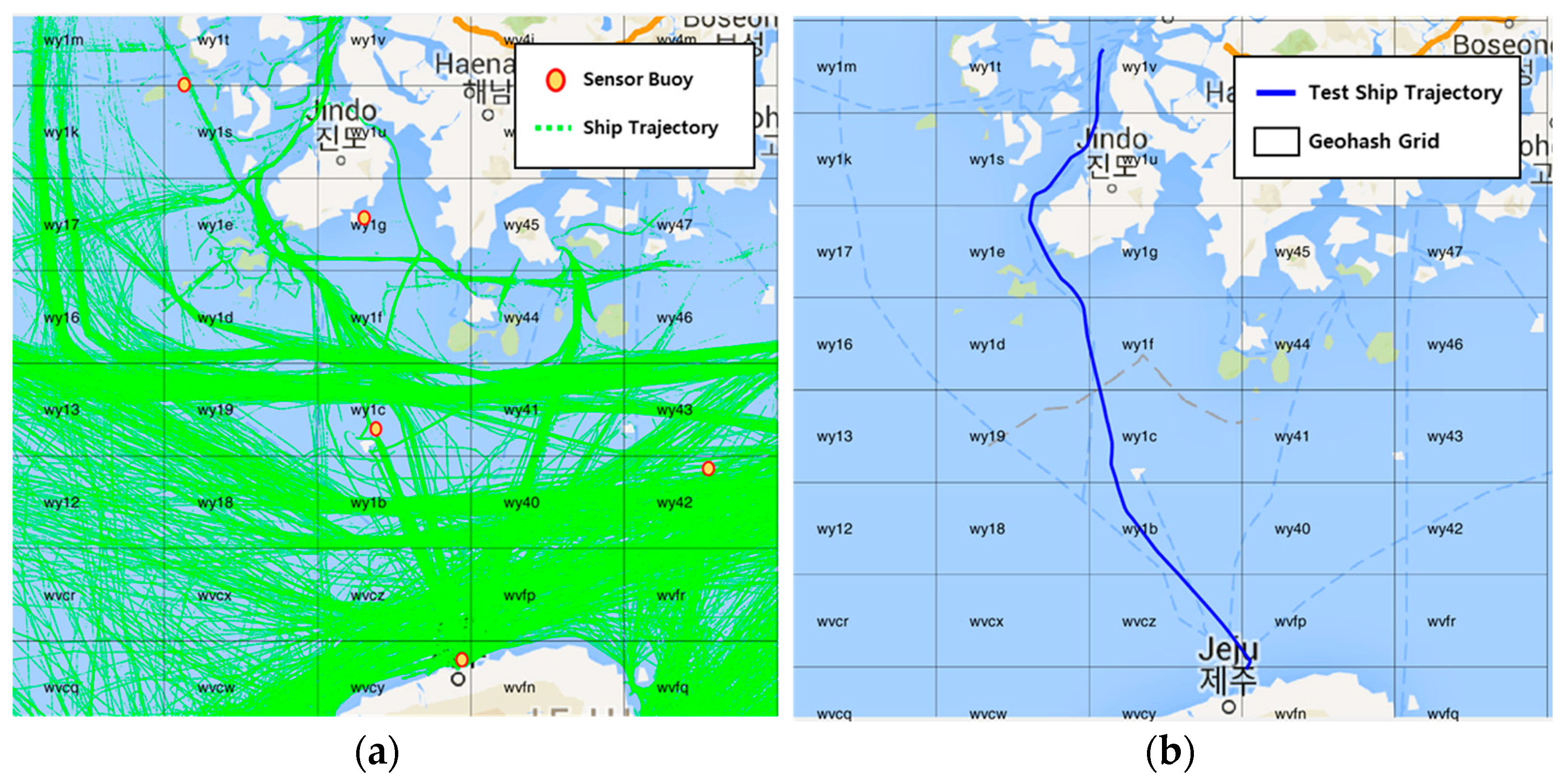
To evaluate the applicability of the proposed DP-based optimal speed adjustment method, we applied it to a real dataset. For the experiments, we collected the vessel traffic data and marine environmental data for the southwestern sea of the Korean Peninsula in 2016 (Figure 5). Figure 5a shows the trajectories from the vessel traffic data and the locations of sensor buoys that collect tidal current, wave, and wind data. Figure 5b shows a liner route of 82 nautical miles between Jeju and Mokpo, which are the ports in the region; the proposed DP-based optimal speed adjustment method was applied to this route. In the figures, the grids correspond to Geohash level 4 grids.

In the study area, the number of sensor buoys is limited, and available sensor values were interpolated to provide environmental data for grids with no sensor buoys (Figure 5a). For each traffic data point to travel a route, the environmental data were acquired or interpolated from the marine environmental database, and their corresponding key-value pairs and speed changes were stored into the externally forced speed-change database. When searching for an optimal speed adjustment plan, the externally forced speed-change information was retrieved by referring to the reference ship, the environmental situation, and the vessel position.

The first experiment was conducted for a towing vessel that travels at a speed of 8 kt and for a general cargo ship that travels at 11 kt on the route shown in Figure 5b. The towing vessel travels the route while pushing a barge carrying large volumes of sand. A SOW of 8 kt is slow for oceangoing voyages, and the effective speed, that is, SOG, is strongly affected by external forces. A SOW of 11 kt is normal for a general cargo ship to navigate in the ocean. We considered these two cases to understand how the efficiency of the proposed DP-based method changes with navigation speed.

Figure 6 shows the experimental results in terms of the SOW, externally forced speed changes experimented by the vessel, and SOG. In Figure 6, “base” indicates fixed-speed navigation and “DP” indicates the navigation for which the speed was adjusted according to the plan, that is, the DP-based method recommended. For the first voyage of 8 kt SOW, the DP-based method changed the vessel speed from 6.5 to 9 kt, while the base method fixed the speed to 8 kt. Figure 7 shows the energy consumption and the average of the externally forced speeds for the fixed-speed navigation and the speed adjustment navigation in the two vessels. The DP-based method found an optimal speed adjustment plan that saved energy. Energy savings came from the effective use of externally forced speeds. The DP-based method recommended a plan that suggested large externally forced speed changes in the positive direction that helped the vessel move quickly rather than with fixed-speed navigation (Figure 7).

To evaluate the emission reductions associated with the DP-based speed adjustment method, we conducted experiments in navigation environments with low, medium, and high external forces at six different baseline speeds from 6 to 13 kt.

Table 6. Energy saving and emission reductions.

Case	Reference Speed	Reference Speed Energy	DP Speed Energy	Energy Savings (KWh)	Shipping Emission Savings (g)
					PM	$\mathbf{N}{\mathbf{O}}_{\mathbf{x}}$	$\mathbf{S}{\mathbf{O}}_{\mathbf{x}}$	CO	HC	$\mathbf{C}{\mathbf{O}}_2$	$\mathbf{C}{\mathbf{H}}_4$	${\mathbf{N}}_2\mathbf{O}$
Marine environment case 1 (low external forces)	8	3025.8	2702.1	323.8 (10.7%)	319	4209	2085	356	162	221,126	3.2	10.0
	9	3015.7	2681.1	334.5 (11.1%)	329	4349	2154	368	167	228,492	3.3	10.4
	10	2985.3	2697.0	288.3 (9.5%)	284	3747	1856	317	144	196,882	2.9	8.9
	11	3003.3	2845.0	158.3 (5.2%)	156	2058	1019	174	79	108,110	1.6	4.9
	12	3025.8	2986.5	39.3 (1.3%)	39	511	253	43	20	26,870	0.4	1.2
	13	3029.2	3006.5	22.7 (0.8%)	22	296	146	25	11	15,530	0.2	0.7
Marine environment case 2 (medium external forces)	8	3025.8	2922.7	103.1 (3.4%)	101	1341	664	113	52	70,447	1.0	3.2
	9	3015.7	2936.1	79.6 (2.6%)	78	1035	513	88	40	54,360	0.8	2.5
	10	2985.3	2834.9	150.4 (5.0%)	148	1955	969	165	75	102,737	1.5	4.7
	11	3003.3	2902.0	101.3 (3.3%)	100	1317	652	111	51	69,177	1.0	3.1
	12	3025.8	2979.8	46.0 (1.5%)	45	598	296	51	23	31,418	0.5	1.4
	13	3029.2	2991.2	38.0 (1.3%)	37	494	245	42	19	25,954	0.4	1.2
Marine environment case 3 (high external forces)	8	3025.8	2270.0	755.8 (25.0%)	744	9826	4868	831	378	516,234	7.6	23.4
	9	3015.7	2381.7	634.0 (21.0%)	624	8242	4083	697	317	433,000	6.3	19.7
	10	2985.3	2400.7	584.6 (19.3%)	575	7600	3765	643	292	399,297	5.8	18.1
	11	3003.3	2386.7	616.6 (20.4%)	607	8016	3971	678	308	421,167	6.2	19.1
	12	3025.8	2605.5	420.3 (13.9%)	414	5465	2707	462	210	287,097	4.2	13.0
	13	3029.2	2765.6	263.6 (8.7%)	259	3427	1698	290	132	180,033	2.6	8.2

shows the energy consumption and emission savings. The DP-based method identified the better-performing plans more so in the high-external-force environment than in the low-external-force environment. In addition, the DP-based method identified an efficient speed adjustment plan at low navigation speeds rather than at high navigation speeds. This means that the DP-based method finds the most efficient plans if the arrival time is not strict.

7. Conclusions

Saving energy and reducing emissions are paramount concerns in transportation and environmental preservation. We propose a DP-based method that recommends optimal speed adjustment plans for navigation routes in response to external forces, unlike the conventional navigation systems. To estimate the externally forced speed changes according to the ship’s condition and position, the proposed method extracts the mapping information from the combined configuration of the ship’s status, marine environmental conditions, and speed changes by analyzing large volumes of AIS and marine environmental data using MapReduce-based operations. The simulation experiments showed that the DP-based method developed speed adjustment plans that produced up to about 20% energy savings under high-external-force conditions. The pollutant emissions were proportional to the energy consumption; thus, the speed adjustment plans determined by the proposed DP-based method also reduced pollutant emissions. The experimental results revealed the emission reductions achieved by the recommended speed adjustment plans. Ships consume large amounts fossil fuel and pose great a threat to the environment. Optimal speed adjustment against external forces can reduce fuel consumption and help to protect the environment.

The proposed DP-based method does not take into account the energy loss caused by speed changes from the following observations. First, the conventional fixed-speed navigation method changes the revolutions per minute (RPM) of the engine because of changing external resistance, which also incurs energy loss at RPM changes. Second, there are some compensation effects for speed acceleration and slowdown: The energy consumption increases at speed acceleration while the inertia of motion helps to save energy consumption at speed slowdown. Third, we have yet no energy consumption model in hand that considers the energy loss due to speed change. Once we have such an energy consumption model, a new DP-based method can be easily developed in a similar way to the proposed DP-based method.

References

- Kattner, L.; Mathieu-Üffing, B.; Burrows, J.P.; Richter, A.; Schmolke, S.; Seyler, A.; Wittrock, F. Monitoring Compliance with Sulfur Content Regulations of Shipping Fuel by in Situ Measurements of Ship Emissions. Atmos. Chem. Phys. 2015, 15, 10087–10092. [Google Scholar] [CrossRef]
- Lam, J.S.L.; Lai, K.H. Developing Environmental Sustainability by ANP-QFD approach: The case of Shipping Operations. J. Clean. Prod. 2015, 105, 275–284. [Google Scholar] [CrossRef]
- Kim, J.S.; Jeong, J.S. Extraction of Reference Seaway through Machine Learning of Ship Navigational Data and Trajectory. Int. J. Fuzzy Log. Intell. Syst. 2017, 17, 82–90. [Google Scholar] [CrossRef]
- Bhardwaj, S.; Ozcelebi, T.; Lukkien, J.J.; Lee, K.M. Semantic Interoperability Architecture for Smart Spaces. Int. J. Fuzzy Log. Intell. Syst. 2018, 1, 50–57. [Google Scholar] [CrossRef]
- Kim, K.I.; Lee, K.M. Ship Encounter Risk Evaluation for Coastal Areas with Holistic Maritime Traffic Data Analysis. Adv. Sci. Lett. 2017, 23, 9565–9569. [Google Scholar] [CrossRef]
- Hanssen, G.L.; James, R.W. Optimum ship routing. J. Navig. 1960, 13, 253–272. [Google Scholar] [CrossRef]
- Hagiwara, H. Weather Routing of Sail Assisted Motor Vessels. Ph.D. Thesis, Technical University of Delft, Delft, The Netherlands, 1989. [Google Scholar]
- Jeong, J.S.; Rhyu, K.S. A study on the Optimal Navigation Route Decision using A* algorithm. J. Korean Inst. Off. Autom. 1999, 4, 38–46. [Google Scholar]
- Zhang, J.; Huang, L. Optimal Ship Weather Routing Using Isochrone Method on the Basis of Weather Changes. In Proceedings of the International Conference on Transportation Engineering, Chengdu, China, 22–24 July 2007; Volume 1, pp. 2650–2655. [Google Scholar]
- Choi, K.S.; Park, M.K.; Lee, J.H.; Park, G.I. A study on the Optimum Navigation Route Safety Assessment System using Real Time Weather Forecasting. J. Korean Soc. Mar. Environ. Saf. 2007, 13, 133–140. [Google Scholar]
- Wang, K.; Yan, X.; Yuan, Y.; Li, F. Real-time optimization of ship energy efficiency based on the prediction technology of working condition. Transp. Res. Part D Transp. Environ. 2016, 46, 81–93. [Google Scholar] [CrossRef]
- Du, Y.; Chen, Q.; Lam, J.S.L.; Xu, Y.; Cao, J.X. Modeling the impacts of tides and the virtual arrival policy in berth allocation. Transp. Sci. 2015, 49, 939–956. [Google Scholar] [CrossRef]
- Oil Companies International Marine Forum (OCIMF). Virtual Arrival: Optimizing Voyage Management and Reducing Vessel Emissions—An Emissions Management Framework; Oil Companies International Marine Forum (OCIMF): London, UK, 2010. [Google Scholar]
- Dulebenets, M.A.; Moses, R.; Ozguven, E.E.; Vanli, A. Minimizing Carbon Dioxide Emissions Due to Container Handling at Marine Container Terminals via Hybrid Evolutionary Algorithms. IEEE Access 2017, 5, 8131–8147. [Google Scholar] [CrossRef]
- Browning, L.; Bailey, K. Current Methodologies and Best Practices for Preparing Port Emission. In Proceedings of the 15th International Emission Inventory Conference, New Orleans, LA, USA, 15–18 May 2006. [Google Scholar]
- Yin, Y.; Lam, J.S.L.; Tran, N.K. Review of Emission Accounting Models in the Maritime Industry. In Proceedings of the 40th IAEE International Conference Meeting the Energy Demands of Emerging Economies, Singapore, 18–21 June 2017; International Association for Energy Economics: Cleveland, OH, USA, 2017. [Google Scholar]
- Huang, L.; Bae, Y.C. Periodic Doubling and Chaotic Attractor in the Love Model with a Fourier Series Function as External Force. Int. J. Fuzzy Log. Intell. Syst. 2017, 17, 17–25. [Google Scholar] [CrossRef]
- Brian, G.; Gareth, W.; Duncan, R.J.S.; David, M.I.; Vengatesan, V. Characterization of Tidal Flows at the European Marine Energy Centre in the Absence of Ocean Waves. Energies 2018, 11, 176. [Google Scholar]
- Eva, S.; Rafael, M.; José, A.S. Cost Assessment Methodology and Economic Viability of Tidal Energy Projects. Energies 2017, 10, 1806. [Google Scholar]
- Kim, K.I.; Lee, K.M. Context-Aware Information Provisioning for Vessel Traffic Service Using Rule-Based and Deep Learning Techniques. Int. J. Fuzzy Log. Intell. Syst. 2018, 18, 13–19. [Google Scholar] [CrossRef]
- Shvachko, K.; Kuang, H.; Radia, S.; Chansler, R. The Hadoop Distributed File System. In Mass Storage Systems and Technologies (MSST). In Proceedings of the 2010 IEEE 26th symposium on IEEE 2010, Incline Village, NV, USA, 3–7 May 2010; Volume 1, pp. 1–10. [Google Scholar]
- International Maritime Organization (IMO). Guidelines for the Onboard Operational Use of Shipborne Automatic Identification Systems (AIS); Res A.917; International Maritime Organization (IMO): London, UK, 2002. [Google Scholar]
- Fox, A.; Eichelberger, C.; Hughes, J.; Lyon, S. Spatio-temporal indexing in non-relational distributed databases. In Proceedings of the 2013 IEEE International Conference on Big Data, Silicon Valley, CA, USA, 6–9 October 2013; Volume 1, pp. 291–299. [Google Scholar]
- Dean, J.; Ghemawat, S. MapReduce: Simplified data processing on large clusters. Commun. ACM 2008, 51, 107–113. [Google Scholar] [CrossRef]
- Korean Register. Available online: http://www.krs.co.kr/kor/ship_as_address/regist_search.aspx?s_code=0505010000 (accessed on 16 April 2018).
- Korean Port Management Information System. Available online: https://new.portmis.go.kr/portmis (accessed on 16 April 2018).
- Zhou, J.; Zhou, S.; Zhu, Y. Characterization of Particle and Gaseous Emissions from Marine Diesel Engines with Different Fuels and Impact of After-Treatment Technology. Energies 2017, 10, 1110. [Google Scholar]
- Han, J.; Charpentier, J.F.; Tang, T. An Energy Management System of a Fuel Cell/Battery Hybrid Boat. Energies 2014, 7, 2799–2820. [Google Scholar] [CrossRef] [Green Version]
- Cormen, T.H. Introduction to Algorithms, 3rd ed.; The MIT Press: Cambridge, MA, USA, 2009; pp. 359–413. [Google Scholar]
- Cho, Y.G.; Lee, H.J. A Position and Velocity Estimation Using Multifarious and Multiple Sensor Fusion. Int. J. Fuzzy Log. Intell. Syst. 2017, 17, 121–128. [Google Scholar] [CrossRef]
Figure 1.
Process of extracting externally forced speed changes from ship data and marine environmental sensor data using MapReduce operations.
Figure 2.
MapReduce operations for extracting externally forced speed changes.
Figure 3.
Information sources and emission quantity estimation.
Figure 4.
Relationship between the accumulated energy consumption and energy consumption by traveling to adjacent points.
Figure 5.
The southwestern sea of the Korean Peninsula for which the experimental data was collected. (a) Ship trajectories of traffic data and the location of sensor buoys used to collect the marine environmental data; (b) a liner route for optimal speed adjustments.
Figure 6.
Speeds over water (SOWs), externally forced speed changes, and speed over ground (SOG) for fixed-speed navigation and dynamic programming (DP)-based speed adjustment navigation. (a) A towing vessel of 8 kt SOW; (b) a cargo vessel of 11 kt SOW.
Figure 7.
The energy consumption and the average of externally forced speeds for the fixed-speed navigation and the dynamic programming (DP)-based speed adjustment navigation. (a) A towing vessel of 8 kt speed over water (SOW); (b) a cargo vessel of 11 kt SOW.