A Fault Isolation Method via Classification and Regression Tree-Based Variable Ranking for Drum-Type Steam Boiler in Thermal Power Plant

Abstract

Accurate detection and isolation of possible faults are indispensable for operating complex industrial processes more safely, effectively, and economically. In this paper, we propose a fault isolation method for steam boilers in thermal power plants via classification and regression tree (CART)-based variable ranking. In the proposed method, binary classification trees are constructed by applying the CART algorithm to a training dataset which is composed of normal and faulty samples for classifier learning then, to perform faulty variable isolation, variable importance values for each input variable are extracted from the constructed trees. The importance values for non-faulty variables are not influenced by faulty variables, because the values are extracted from the trees with decision boundaries only in the original input space; the proposed method does not suffer from smearing effect. Furthermore, the proposed method, based on the nonparametric CART classifier, can be applicable to nonlinear processes. To confirm the effectiveness, the proposed and comparison methods are applied to two benchmark problems and 250 MW drum-type steam boiler. Experimental results show that the proposed method isolates faulty variables more clearly without the smearing effect than the comparison methods.

1. Introduction

Modern industrial processes (e.g., power plants, and chemical and manufacturing processes) are becoming larger and more complex owing to efforts to fulfill safety and environmental regulations, to save costs, and to maximize profits. Therefore, process monitoring for accurate and timely detection and isolation of potential faults is more important than ever before. Faults are defined as abnormal events that occur during process operations. In thermal power plants (TPPs), main generating units (e.g., steam boilers and turbines) operate under very high pressure and temperature; if possible faults of the main units are not detected and isolated precisely, they may result in system failures, and eventually may cause significant losses of life and property. Properly designed monitoring systems can ensure safe, effective, and economical operations of target processes.

Statistical process monitoring techniques fall into two categories: model-based and data-based methods. In the model-based methods, process monitoring is carried out by rigorous mathematical models derived from prior physical and/or chemical knowledge (e.g., mass or energy balances) governing target processes; the monitoring performance may be degraded when the derived models are inaccurate. If target processes are heavily complex and large-scale, the derivation of the models is difficult, or may be impossible; even when possible, it is costly and takes much time. Despite their development efforts (e.g., mathematical derivations and proofs), they may be limited by boundary conditions for specific system behaviors or only applicable for particular system setups [1]. In the data-driven techniques, monitoring models are developed based on historical operation data. Recent advances in communications and measurement technologies facilitate the installation of huge numbers of sensors in target processes; various key variables related to process monitoring and control are measured by the installed sensors. Distributed control systems and/or supervisory control and data acquisition systems built into modern industrial processes enable efficient management and storage of the massive amounts of operational data. Without mathematical models based on the first-principles, the data-driven methods are capable of extracting useful health information from abundant operation data; they are receiving a great deal of attention from academia and industries.

Process monitoring is carried out via the following four steps [2]: fault detection, fault isolation, fault diagnosis, and process recovery. Fault detection determines whether possible faults have occurred; early detection helps operators and maintenance personnel take corrective actions to prevent developing abnormal events from leading to serious process upsets. Fault isolation (also called fault identification) locates faulty variables closely related to detected faults; the isolation results assist field experts in diagnosing the faults precisely, i.e., it helps the system operators to determine which parts should be repaired or replaced [3]. Fault diagnosis investigates the root causes and/or sources of occurring faults. Process recovery corresponds to the last step in finishing the process monitoring loop; in this step, the effects of abnormal events are removed and target processes get back to normal operating conditions.

So far, multivariate statistical techniques and machine learning have been widely used for fault detection and diagnosis of power plant equipment, such as principal component analysis (PCA) [4,5,6,7], independent component analysis (ICA) [8,9], auto-associative kernel regression (AAKR) [10,11], artificial neural networks [12,13], fuzzy models [14,15], support vector machine [15,16], neuro-fuzzy networks [17], and group method of data handling [18]. PCA and ICA can handle multivariate process data effectively via dimensionality reduction. AAKR is a nonparametric multivariate technique to obtain predicted vectors for new query vectors by updating local models in real time; it can perform fault detection tasks without any assumptions for target data properties (e.g., linear or nonlinear). In the case of machine learning techniques for black box modeling, considering nonlinearities of target processes, fault detection and diagnosis can be carried out without the need of physical or chemical knowledge. Although these methods can detect potential faults successfully, they may have several difficulties in isolating and diagnosing the faults.

As explained above, after the fault detection tasks, fault isolation and diagnosis should be conducted to pinpoint the root causes of occurring faults. If there exist abundant historical faulty samples whose class labels are associated with all possible fault categories, multi-class classifiers [19,20,21,22] can be explicitly constructed. The designed classifiers assign the most similar fault categories to query samples; faults are diagnosed without the fault isolation procedure. When designing such classifiers, one might face the following difficulties. First, in general, the number of available faulty samples is much fewer than that of normal samples. Actual industrial processes are carefully designed to prevent abnormal events; the processes are equipped with closed-loop controllers compensating for the effects of unpermitted changes and disturbances. In addition, to build multi-class classification models, preparing complete training dataset encompassing all types of faults is nearly impossible; if all possible faults occurred several times in the past and the corresponding fault dataset was stored in a database, or if there are useful simulators that can emulate target processes as perfectly as possible, collecting the complete dataset may be possible. Second, collected training dataset for classifier learning is usually class-imbalanced [23]; the number of faulty samples may vary from class to class considerably. Furthermore, high levels of expert experience and knowledge are required to assign proper class labels to historical faulty samples; these labeling procedures may also be time-consuming. Lastly, classifiers based only on historical fault data do not function adequately when new types of faults develop.

When the faulty data samples encompassing all possible fault types are not enough, after isolating faulty variables based on detection indices from fault detection models, the isolation results can be used for fault diagnosis. In the fault detection models, normal samples are only needed for training, and whether target processes fall outside normal operating regions is decided in real time; if detection indices for query samples deviate from predefined threshold values, fault occurrence is declared, and alarm signals are generated. After faults are detected, fault isolation should be performed to determine which variables are responsible for the detected faults. Contribution plots [24,25] are the most popular method for fault isolation; it is assumed that the contribution values of faulty variables to detection indices are higher than those of non-faulty ones. In this method, monitored variables are identified as faulty variables if their contribution values violate the confidence limits. Although the contribution analysis can identify faulty variables quickly and easily without a historical fault dataset and prior information on possible fault types, it has several limitations, as follows: first, the threshold values derived only from normal data may be unsuitable for isolating faulty variables, because contribution values of each variable within in-control regions may follow different distributions from those outside the regions. Second, it is well-known that isolation results from contribution plots confuse process operators and engineers due to the smearing effect [26,27,28]; smearing is a phenomenon that contribution values of non-faulty variables are enlarged by faulty variables. When complicated faults, rather than simple faults, have happened, fault isolation with contribution analysis may lead to an ambiguous diagnosis.

In this paper, we propose a fault isolation method via classification and regression tree (CART)-based variable ranking for a drum-type steam boiler in TPP; it is assumed that some proper fault detection algorithms were already designed, and after possible faults are detected by the algorithms, the proposed fault isolation method is triggered. CART algorithm [29] with a divide-and-conquer mechanism, splits the entire input space repeatedly and builds binary trees. CART has been successfully applied to various fields [30,31,32,33] for which data mining techniques are necessary, since it can tackle multivariate data efficiently, and the constructed trees are transparent. In the proposed method, after designing classification trees by applying CART algorithm to training dataset composed of normal and faulty samples, variable ranking is performed by extracting importance values of each input variable from the trees. In the training dataset, Normal and Abnormal class labels are assigned to the normal and faulty samples, respectively; the faulty samples are relevant to the regions where the detection indices are larger than or equal to threshold values. In this paper, as will be explained in Section 3, we propose two approaches (see Figure 1) for fault isolation; the goal of the first approach is to locate faulty variables in entire fault regions, and the second approach (with time window sliding) aims to monitor how occurring faults propagate and evolve.

The proposed method, based on the nonparametric CART algorithm, can be applicable to fault isolation of nonlinear processes; the method can locate faulty variables even when normal and faulty samples cannot be linearly separated from each other. Above all, the proposed isolation method does not suffer from the smearing effect, since it is based on CART algorithm defining decision boundaries only in the original input space. To verify the performance, the proposed method and comparison methods are applied to two benchmark problems and a 250 MW drum-type steam boiler. Experimental results show that the proposed method can effectively identify faulty variables without suffering from fault smearing, and can properly tackle nonlinearities of target processes.

The remainder of this paper is organized as follows: Section 2 explains CART-based tree growing, pruning, and variable ranking. Section 3 describes the proposed isolation method via the variable ranking. Section 4 presents the experimental results and discussion, and finally, we give our conclusions in Section 5.

2. Classification and Regression Tree

The CART algorithm [29] builds binary decision trees by recursively dividing a given training dataset into several subsets; the entire input space is partitioned into mutually exclusive rectangular regions. In the constructed trees, nodes without any child nodes are named terminal nodes (i.e., external or leaf nodes); they form a partition of all the training samples. The remaining nodes except for the terminal nodes are called internal nodes, which have only two child nodes; especially, the nodes located at the top of the trees are defined as root nodes. In classification trees, out of several class labels, only one label is assigned to each terminal node.

The advantages of CART algorithm can be summarized as follows [29,34]: first, without any prior domain knowledge, classifiers can be constructed only from input-output training dataset; multivariate data collected from complex target systems can be efficiently handled by its divide-and-conquer approach. Second, one does not need to be concerned about target data properties in advance (e.g., linear or nonlinear) because of its nonparametric nature. Third, the algorithm is robust against statistical outliers and mislabeled training samples. Lastly, final tree structures and if-then rules taken from the trees explicitly describe predictive principles of target problems; one can clearly understand how the classification procedures are conducted by the trees. The following CART-based tree growing, pruning, and variable ranking steps explained in Section 2.1, Section 2.2 and Section 2.3 are based on [29].

2.1. Tree Growing

In the CART algorithm, splitting a note t into two child nodes, t_L and t_R, is achieved by selecting an optimum binary split point that makes the child nodes purer than the parent node; here, the subscripts L and R denote Left and Right, respectively. There are several criteria (i.e., impurity function i(t)), such as Gini diversity index, cross entropy, and twoing rule, used for impurity measures; in [29], it was reported that the properties of constructed trees do not depend highly on the types of criteria. In this study, to measure node impurities, we use Gini diversity index defined as:

$$i(t)={\displaystyle \sum _{l\ne k}p(l|t)p(k|t)}={\left({\displaystyle {\sum }_{l}p(l|t)}\right)}^2-{\displaystyle {\sum }_l{p}^2(l|t)}=1-{\displaystyle {\sum }_l{p}^2(l|t)}, l, k=1, \dots , C,$$

(1)

where C is the number of assignable class labels, and p(l|t) is the ratio of samples with lth class label among all samples at node t, i.e., ${\mathsf{\Sigma }}_{l=1}^{C}p(l|t)=1$. In two-class problems (i.e., C = 2), Equation (1) can be rewritten as i(t) = 2p(1|t)p(2|t). In (1), the cost, c(k|l), k ≠ l, of misclassifying a sample with lth label into kth label is set to 1; the cost may vary from label to label. Gini diversity index with c(k|l) ≠ 1, k ≠ l, is calculated as:

$$i(t)={\displaystyle \sum _{l,k}c(k|l)p(k|t)p(l|t)},$$

(2)

where c(k|l) = 0 for k = l. In two-class problems, Equation (2) can be written as i(t) = (c(2|1) + c(1|2))p(1|t)p(2|t).

Let s denote a candidate split point dividing a node t into t_L and t_R, and let p_L and p_R be the ratios of training samples entering t_L and t_R, respectively, by the split point among all samples at node t. The candidate split points of jth continuous input variable x_j are obtained from averaging all possible adjacent pairs of training samples with respect to x_j. The goodness of split point s at node t, Δi(s, t), is defined as a decrease in impurity:

$$\Delta i(s,t)=i(t)-p_{L}i(t_L)-p_{R}i(t_R).$$

(3)

Let S be a set that consists of all possible candidate split points for all input variables. The best split point s^* that gives the largest decrease in impurity is obtained by:

$$s^{\ast }=\underset{s\in S}{\arg \max }\Delta i(s,t).$$

(4)

For example, when the split point s^* divides a node t into t_L and t_R on the j^*th input variable $x_{j^{\ast }}$, training samples belonging to t_L and t_R are satisfied with the conditions $x_{j^{\ast }}<s^{\ast }$ and $x_{j^{\ast }}\ge s^{\ast }$, respectively.

By the above principles, root node t₁ is split into descendant nodes t₂ and t₃, and then, partitioning is continuously applied at each node separately. If $\Delta i(s^{\ast },t)$ is smaller than a predefined value, then node splitting is stopped and the node t is regarded as a terminal node; the class label of the terminal node can be determined by plurality rule [29].

2.2. Tree Pruning

In tree growing, it may be unhelpful for the performance of final trees to consider complicated rules for stopping node division. Instead of stopping node splits when reaching a tree with right-sized terminal nodes, after continuing the splits until the number of training samples at each terminal node is very small (i.e., constructing a very large tree with many terminal nodes), it is much better to decide the final tree structure through selective upward pruning. A decreasing sequence of subtrees can be obtained by applying sequential tree pruning to the large tree in the direction of the root node; the tree with the minimum misclassification rate can be finally selected from the subtrees. In this paper, after obtaining the sequence of subtrees through minimal cost-complexity pruning, the final trees with optimal number of terminal nodes are selected using cross-validation. This recursive pruning process is computationally efficient; this process requires only a small fraction of the total tree construction time [29].

2.3. Variable Ranking Based on Surrogate Splits

Assume that node t is divided into t_L and t_R by best split point s^* on best split variable $x_{j^{\ast }}$. Surrogate splits are defined as split points that behave most similarly to s^* on the remaining input variables, except for $x_{j^{\ast }}$. Suppose that node t can also be partitioned into ${t^{\prime }}_L$ and ${t^{\prime }}_R$ by candidate splits s_j on input variables x_j, j $\in$ {1, …, m}\j^*. Let N_LL(t) and N_RR(t) be the number of training samples going to the left and right nodes by both s^* and s_j, respectively; N_LL(t) and N_RR(t) are the number of samples that meet the conditions $x_{j^{\ast }}$ < s^* and x_j < s_j, and the conditions $x_{j^{\ast }}$ ≥ s^* and x_j ≥ s_j, respectively. The probability that s_j correctly predicts the action of s^* is defined as:

$$p(s_j,s^{\ast })=\frac{N_{LL}(t)+N_{RR}(t)}{N(t)},$$

(5)

where N(t) is the number of training samples belonging to node t. If the probability values are larger, s_j closely mimics s^*; if s^* sends a sample to t_L, then the likelihood of s_j sending the sample to ${t^{\prime }}_L$ is high. The best surrogate split ${\tilde{s}}_j$ on x_j can be obtained through:

$${\tilde{s}}_j=\underset{s_j}{\arg \max }p(s_j,s^{\ast }).$$

(6)

If there are no split points on some input variables in final trees, we may think that these variables are useless for classification; however, this is a misinterpretation of the final trees when the effects of the variables are masked by other variables. In other words, although node splits on some variables do not appear in the final trees, the importance of those variables may be high; this may be the evidence of the masking. For example, for convenience of explanation, let us assume that two input variables x₁ and x₂ have greater effects on classification than other variables; here, the effects of x₁ and x₂ are similar but the effect of x₁ is a little larger than that of x₂. In this case, node splits may be performed only on the masking variable x₁ (i.e., x₂ may be masked by x₁); if x₁ is removed, x₂ may be prominently used as split variable. In summary, under the above situations, instead of determining variable importance only by examining split variables in final tree structures, we should decide variable importance through the variable ranking based on the surrogate splits [29]. The masking may occur when input variables are highly correlated to each other. For CART users, it is essential to confirm which variables are the most significant for classification and to rank variables according to their importance. Based on the surrogate splits explained above, one can calculate the importance values of each input variable. After calculating the goodness of split Δi(s, t) for best split s^* and surrogate splits ${\tilde{s}}_j$ relevant to all input variables at all internal nodes, the importance of the jth variable can be measured by:

$$M(x_j)={\displaystyle \sum _{t\in T^{\prime }}\Delta i(s,t)p(t)},$$

(7)

where T′ is a set composed of all internal nodes in the final trees, and p(t) is the ratio of samples at node t to entire training samples. If x_j corresponds to the best split variable at node t, then the best split s^* is substituted into Equation (7) (i.e., in Equation (7), Δi(s, t) ≡ Δi(s^*, t)); otherwise, the value of s takes surrogate splits ${\tilde{s}}_j$ of x_j instead of s^* (i.e., in Equation (7), Δi(s, t) ≡ $\Delta i({\tilde{s}}_j,t)$). Since we are usually interested in the relative importance of input variables, variable ranking is performed through the normalized importance values as follows:

$$\overline{M}(x_j)=100M(x_j)/\underset{j}{\max }M(x_j).$$

(8)

After extracting variable importance values via Equation (8) from constructed trees, faulty variables can be isolated by comparing these values. In the fault region, faulty variables have great explanatory powers to discriminate normal and faulty samples; their importance values are nearly 100 (i.e., $\overline{M}(x_j)\approx 100$). On the other hand, the values of non-faulty variables are much smaller than those of faulty. In this paper, we decide monitoring variables whose importance values are larger than 80 (i.e., $\overline{M}(x_j)\ge 80$) as faulty variables. After sorting monitoring variables according to their importance values, we can also confirm the priority of variables responsible for occurring faults.

3. CART-Based Fault Isolation

This section provides the proposed fault isolation method via CART-based variable ranking as explained in Section 2.3. The purpose of fault isolation is to identify which monitored variables are closely related to occurring faults, and then to support process operators and engineers in deciding on correct fault types. In this paper, two kinds of approaches are employed for fault isolation. In the first approach, we check how much each variable contributes to the occurring faults in the entire fault region. In the second approach, time window sliding is used to track how the faults evolve and propagate over time. The first approach is suited to offline analysis of process anomalies; the second approach aids in understanding fault evolution and propagation mechanisms online. Figure 1a,b describe the proposed first and second fault isolation approaches, respectively.

From now on, let us take a close look at the first approach (see Figure 1a). In Step 1, we prepare normal data matrix X^normal composed of normal samples $x(t_{\mathrm{start}}^{\mathrm{normal}})$, …, $x(t_{\mathrm{end}}^{\mathrm{normal}})$, and fault data matrix X^fault composed of fault samples $x(t_{\mathrm{start}}^{\mathrm{fault}})$,…, $x(t_{\mathrm{end}}^{\mathrm{fault}})$. The normal samples may correspond to training samples used to build fault detection models such as PCA and ICA; the fault samples are brought from a fault region where alarm signals are consistently generated. And then, training matrix X for tree construction is organized by augmenting X^normal and X^fault; class labels (Normal or Abnormal) are assigned to the last column in X, based on whether input vectors are normal or faulty. Finally, after building a classification tree based on X, the importance values of each variable are calculated, as explained in Section 2.3. In Step 3, after constructing a large tree with many terminal nodes, a sequence of subtrees is obtained through the minimal cost-complexity pruning; then, the optimal tree is selected by cross-validation, and the importance values are computed by Equation (8). The input variables with high importance values are dominant to separate normal and faulty samples in the original input space; they have great explanatory powers when classifying normal and faulty samples. The importance values of non-faulty variables are small, because their behaviors are similar in both normal and fault regions. On the other hand, faulty variables have high importance values, since their patterns are significantly different in the two regions. In summary, the first approach identifies the input variables with high importance values as faulty variables in the entire fault region. This approach cannot confirm how faults evolve and propagate from start time $t_{\mathrm{start}}^{\mathrm{fault}}$ to end time $t_{\mathrm{end}}^{\mathrm{fault}}$.

In the second approach in Figure 1b, calculations of the importance values are repeated by sliding time window with size w along the time axis, i.e., from $t_{\mathrm{start}}^{\mathrm{fault}}$ to $t_{\mathrm{end}}^{\mathrm{fault}}$. The matrix X^fault, composed of w fault samples, changes every moment; except for this, the remaining procedures are same as those of the first approach. For example, at time t = $t_{\mathrm{start}}^{\mathrm{fault}}$ + w − 1, X^fault consists of faulty samples $x(t_{\mathrm{start}}^{\mathrm{fault}})$, …, $x(t_{\mathrm{end}}^{\mathrm{fault}}+w-1)$, and at time t = $t_{\mathrm{start}}^{\mathrm{fault}}$ + w, X^fault consists of faulty samples $x(t_{\mathrm{start}}^{\mathrm{fault}}+1)$, …, $x(t_{\mathrm{end}}^{\mathrm{fault}}+w)$, and so on. Whenever X^fault changes, a new tree should be constructed and variable importance values are extracted from the newly constructed tree; computation time in this approach is longer than the first approach because many final trees are constructed. In this case, to save time, the pruning process may be skipped; the importance values before and after the process may not be considerably different. The importance values obtained through the window sliding from time t = $t_{\mathrm{start}}^{\mathrm{fault}}$+ w − 1 to t = $t_{\mathrm{end}}^{\mathrm{fault}}$ enable proper monitoring of fault evolution and propagation effects. From now on, for convenience of explanation, the two approaches presented in Figure 1a,b are referred to as Method 1 and Method 2, respectively.

4. Experimental Results and Discussion

In this section, to verify the performance, the proposed method (i.e., Method 1 and Method 2) is applied to two benchmark problems (i.e., a simple linear process and a three variable nonlinear process), and 250 MW drum-type steam boiler. In the first and third problems, contribution plots based on PCA and AAKR are employed as comparison methods; in the nonlinear process, since PCA cannot detect bias and drift faults accurately, it is excluded. Before applying fault detection and isolation methods, each monitored variable is normalized to zero mean and unit variance. In PCA, to reduce dimensions in principal component (PC) subspace, PCs capturing more than 85 percent of variations are only retained; contribution analysis for detection indices (i.e., T² and Q statistics) is performed for fault isolation; kernel density estimation (KDE) [35] is employed to define threshold values for fault detection and contribution analysis. In the case of AAKR [11], squared prediction error (SPE) is used as a detection index, and contribution values of monitored variables for SPE are also calculated; in common with PCA, thresholds for fault detection and contribution analysis are determined by KDE. In both PCA and AAKR, level of significance α is set to 0.01. To construct CART classifiers and to extract variable importance values from the classifiers, we employee the ‘fitctree’ and ‘predictorImportance’ MATLAB functions built into the Statistics and Machine Learning Toolbox; the ‘ksdensity’ function in the same toolbox is used to estimate cumulative distribution functions of detection indices and contribution values via KDE.

Method 1 uses the impurity function in Equation (1) to measure node impurities. To take into account imbalance between normal and abnormal classes, Method 2 employs Equation (2) instead of Equation (1). In the case of Method 2, there are much more samples with Normal class labels than those with Abnormal in the training matrix X (see Figure 1) for CART classifiers. In Equation (2), c(1|2) and c(2|1) denote misclassification costs associated with classifying an abnormal sample into a normal sample and vice versa; for example, c(1|2) and c(2|1) can be set to 10 and 1, respectively. In Method 2, the size of time window w is set to 10.

4.1. Simple Linear Process

First, let us describe the results of applying the proposed and comparison methods to the simple linear process, also used in [28]. Simulation data is obtained from the following multivariate linear system:

$$\left[\begin{array}{c}{x}_1\\ x_2\\ x_3\\ x_4\\ x_5\\ x_6\end{array}\right]=\left[\begin{array}{ccc}-0.1681& 0.2870& -0.2835\\ 0.4354& 0.3812& 0.1455\\ 0.0247& -0.0235& 0.4096\\ -0.1173& -0.1763& 0.4382\\ 0.0825& 0.1398& 0.3204\\ -0.3825& 0.1250& 0.4836\end{array}\right]\left[\begin{array}{c}{s}_1\\ s_2\\ s_3\end{array}\right]+e$$

(9)

where x₁, …, x₆ are directly measurable variables, s₁, …, s₃ are source variables that follow normal distributions with mean of 0 and variances of 1, 0.8, and 0.6, respectively, and e is white noise with mean of 0 and variance of 0.04. From Equation (9), the six monitored variables are calculated through the linear combination of three source variables. To train PCA and AAKR, 3000 samples are generated; these samples are also used to form the normal data matrix X^normal in Figure 1. Faulty samples are obtained through the addition of the term ξf(t), reflecting the effects of anomalies, into normal samples x^*(t) as follows:

$$x(t)=x^{\ast }(t)+\mathsf{\xi }f(t),$$

(10)

where the normal sample x^*(t) at time t is corrupted by ξf(t), and ξ and f(t) denote the fault direction vector and fault magnitude, respectively. In this paper, in common with [28], we consider two types of fault (i.e., simple and multiple faults) to verify the fault isolation performance. In the simple fault, the fault direction vector and its magnitude are set to ξ = [0 0 0 1 0 0]^T and f(t) = 10⁻⁵t², respectively, and 1000 faulty samples are generated. The multiple fault is represented with ξ = [1 0 1 0 0 0]^T and f(t) = 6 × 10⁻⁶t², and the corresponding 1200 faulty samples are also generated.

Figure 2 shows the fault isolation results of the comparison methods and Method 2 (see Figure 1b) for the simple and multiple faults. In the figures related to the comparison methods, if variable contribution values at a certain time are larger than or equal to thresholds, the relevant entries display as black; otherwise, the entries are marked with white. In the figures associated with Method 2, variable importance values at a certain time are indicated through different colors; as the values are close to 100 (or 0), the colors for relevant entries are close to black (or white). The simple and multiple faults start to be detected by PCA and AAKR at about time t = 300; the monitoring charts of PCA and AAKR for fault detection are omitted due to space constraints. As presented in Figure 2, PCA-based contribution plots suffer terribly from smearing effect. In the simple fault, in addition to faulty variable x₄, contribution values of normal variables x₁, x₂, x₃, and x₅ deviate from confidence limits. In the multiple fault, we can confirm severe smearing over non-faulty variables x₂, x₅, and x₆. In AAKR-based contribution analysis, smearing over normal variables appears consistently, although its severity is less than PCA. In the case of Method 2, importance values of non-faulty variables are not equal to zero only in the early stages of the faults. However, faulty variables of the simple and multiple faults are clearly identified after approximately time t = 370. Contrary to comparison methods, as the magnitude of the faults becomes larger over time, importance values of normal variables obtained by Method 2 become closer to zero.

Figure 3 shows variable importance values related to the simple and multiple faults, which are calculated by Method 1 (see Figure 1a). For the simple fault, faulty samples from time t = 301 to t = 1000 constitute the fault data matrix X^fault; for the multiple fault, the matrix X^fault consists of faulty samples from time t = 301 to t = 1200. As shown in the figure, variable importance values of faulty variables are much larger than those of normal (i.e., close to 100); the values of non-faulty variables are close to zero. In other words, in this benchmark problem, Method 1 can locate faulty variables accurately in the entire fault regions.

4.2. Three Variable Nonlinear Process

Second, let us look at the results of fault isolation for the nonlinear process (also used in [36,37]) with three monitored variables and one latent variable described as follows:

$$\begin{array}{l}{x}_1=s+e_1\\ x_2=s^2-3s+e_2\\ x_3=-s^3+3s^2+e_3\end{array}$$

(11)

where x₁, …, x₃ are the monitored variables, s $\in$ [0.01, 2] is the source variable, and e₁, …, e₃ follow independent Gaussian distributions with mean and variance of 0 and 0.01, respectively. We obtain 100 normal samples from Equation (11), used to build fault detection models and to form the normal data matrix X^normal. To validate the performance of fault isolation, two fault cases, where each case is composed of 300 test samples, are generated as follows:

• Case 1: A step change of x₂ by −0.4 was introduced starting from sample 101.
• Case 2: x₁ was linearly increased from sample 101 to 270 by adding 0.01(t − 100) to the x₁ value of each sample in this range, where t is the sample number.

Figure 4 shows the fault isolation results of applying AAKR-based contribution analysis and Method 2 to the two fault cases.

AAKR-based contribution analysis starts to identify the faulty variable x₂ in Case 1 at time t = 101, but its contribution values fluctuate constantly, and alarms are repeatedly generated and halted over time; contribution values of x₂ do not steadily deviate from thresholds but depart from and return to normal regions again and again. Also, smearing over normal variable x₃ is frequently observed. These phenomena may cause confusions to root cause analysis for uncovering the fundamental causes and/or sources of occurring faults. In Case 2, contribution values of faulty variable x₁ consistently violate thresholds from about time t = 160 to 270, but smearing over non-faulty variables x₂ and x₃ becomes larger as the magnitude of the fault increases. With Method 2, the importance values of faulty variables in Cases 1 and 2 are very close to 100 in the fault regions. In Case 1, importance values of non-faulty variables x₁ and x₃ fluctuate widely over time; this is not due to smearing effect but is due to the fact that the fault magnitude is not very large. Although the fault occurred only in faulty variables, to determine decision boundaries for dividing normal and faulty samples in the original input space, non-faulty variables as well as faulty variables are needed when the fault magnitude is small. If the magnitude is large enough, it is possible to establish the boundaries using only faulty variables. In Case 2, the importance values of normal variables are slightly large when the fault magnitude is not large enough; as the magnitude becomes larger, the importance values of non-faulty variables decrease gradually.

Now, let us look more carefully into fault isolation results using Method 1. Figure 5 depicts the results of applying Method 1 into Cases 1 and 2. In Case 1, to construct CART classifiers, faulty samples from time t = 201 to 300 constitute the fault data matrix X^fault in Figure 1a; in Case 2, X^fault is composed of faulty samples from time t = 171 to 270. As can be seen from Figure 5, the importance values of faulty variables are nearly 100; the values of non-faulty variables are relatively smaller than those of faulty. Examining the results for Methods 1 and 2 synthetically may greatly help field experts diagnose developing faults in target processes.

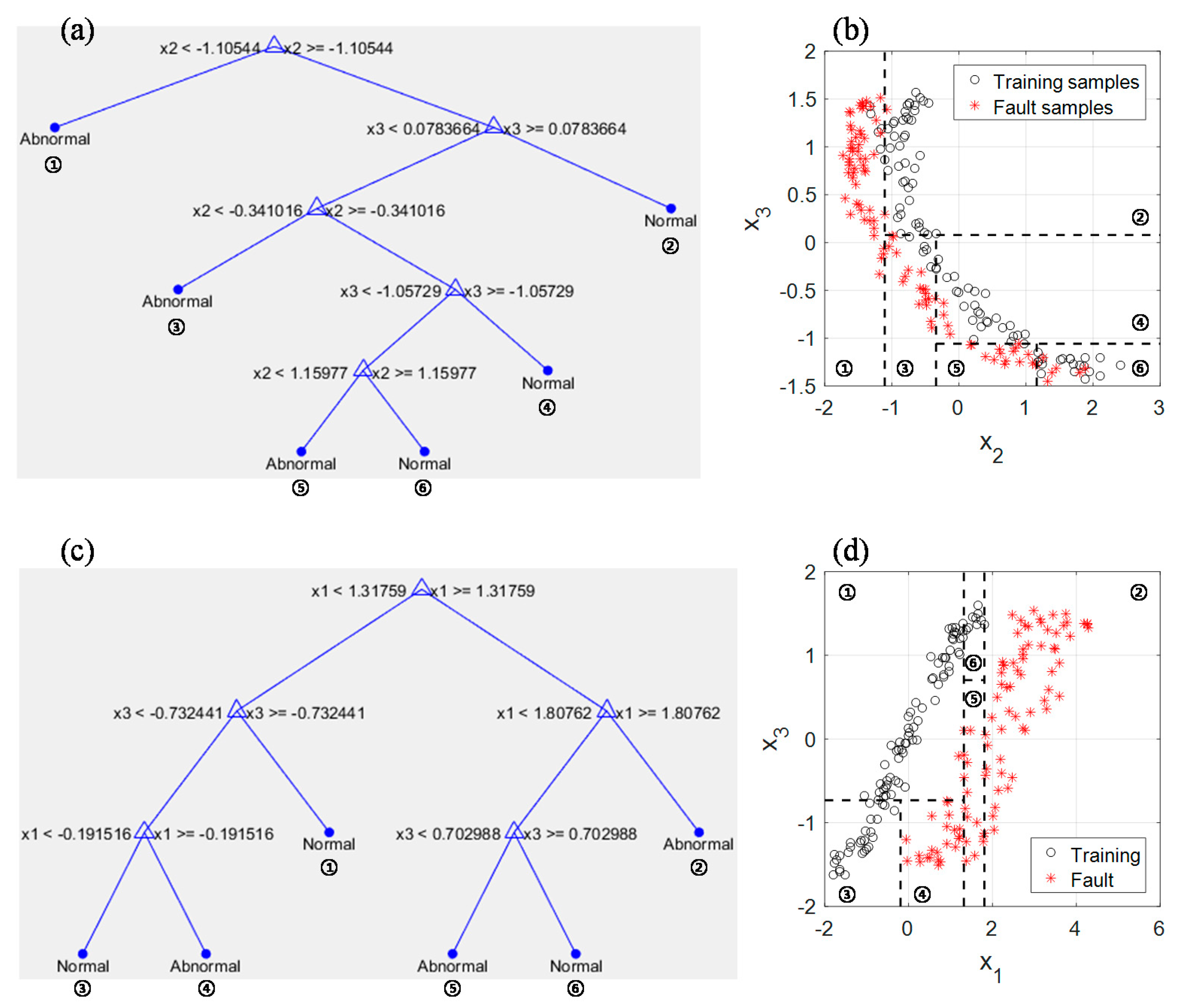
Figure 6 shows the constructed trees from which the importance values in Figure 5 are extracted and the scatter plots for normal and faulty samples used to build the trees.

In Figure 6b,d, normal and faulty samples are denoted by black circles and red asterisks, respectively; faulty samples in Figure 6b,d correspond to samples at time t = 201 to 300 and t = 171 to 270 in Cases 1 and 2, respectively. Index numbers are marked at the bottom of each terminal node in Figure 6a,c, and the corresponding rectangle regions in Figure 6b,d are also indexed by the numbers. In the constructed trees, not only faulty variables but also non-faulty variables have been partitioned; it is important to note that identifying faulty variables via variable importance values in (8) is more reasonable than doing this only through checking split variables in the final trees. In Figure 6b,d, it is obvious that non-faulty variables as well as faulty variables are required to define the decision boundaries for classifying normal and faulty samples. In other words, if the magnitude of mean shifts is small, both faulty and non-faulty variables are needed to derive the boundaries. As the magnitude of the bias and drift faults becomes larger, the need for non-faulty variables shrinks.

4.3. Drum-Type Steam Boiler in Thermal Power Plant

In this subsection, we present the results of applying the proposed fault isolation method to a 250 MW drum-type steam boiler. Figure 7 [11] describes the simplified schematic diagram of the target drum-type boiler.

The boiler raises steam by boiling feedwater using thermal energy converted from fossil fuel. After being preheated by extraction steam from the turbines at feedwater heaters, the feedwater is supplied to the economizer. The feedwater, heated again by flue gas at the economizer, flows into the drum. The feedwater and saturated water in the drum are fed into the evaporator through a downcomer. The evaporator raises saturated steam by absorbing radiant heat of the furnace. The saturated water and steam are separated at the drum. The superheater converts the main steam from the drum into high-purity superheated steam supplied to the high pressure turbine. Working in the high-pressure turbine, the main steam is reheated by reheater and provided to the intermediate pressure turbine. The main steam that exits from the low-pressure turbine is condensed into condensate water. After being boosted by pumps and preheated by feedwater heaters, the water is fed into the boiler again. For more details regarding TPPs, refer to the books of Sarkar [38], Basu and Debnath [39], Kitto and Stultz [40], and Singer [41].

In the target boiler, key process variables such as main steam temperature, furnace pressure, drum water level and condenser make-up flow need to be closely monitored to check whether they deviate from specified limits. For example, main steam temperature may show abnormal variations due to the following several factors: malfunction of attemperators, excess air ratio, fouling formed on outer surfaces of superheater, and slag attached to outer surfaces of waterwall. To avoid the failures due to extremely high metal temperature, it is indispensable to control the steam temperature precisely [6]. When the steam temperature is lower than its rated value, moisture content in the main steam may increase; this may cause erosion of steam turbines. Also, if there are some problems with feedwater supply, drum water level may increase or decrease. The unusual rises of drum level may result in carryover of water into superheaters or steam turbines. On the other hand, if the level is too low, the amount of feedwater supplied into waterwall tubes declines. In this case, the tubes cannot readily absorb radiation energy generated in the furnace; this may reduce the life expectancy of the tubes due to overheating, and may lead to catastrophic disasters.

Table 1. Summary of monitored variables for target drum-type steam boiler.

Variable	Description	Unit
x1	Generator output	MW
x2	Steam flow	t/h
x3	Main steam pressure	kg/cm2
x4	Main steam temperature	°C
x5	Reheater pressure	kg/cm2
x6	Furnace pressure	kg/cm2
x7	Drum level	m
x8	Condenser make-up flow	t/h
x9	Feedwater flow	t/h

lists process variables for condition monitoring of the target boiler in Figure 7.

4.3.1. Artificial Fault Cases

From now on, we describe the results for fault isolation of artificially generated two fault cases in the target boiler. For the simulation study, 2500 historical normal samples from the target system are prepared; each sample is recoded in 5-min intervals. Among the normal samples, 2000 samples are used to train fault detection models (i.e., PCA and AAKR) and to form the normal data matrix X^normal in Figure 1a; the remaining 500 samples are considered as test dataset. In the test dataset, we generate artificial drift and bias faults, respectively, starting at 201th samples as follows:

• Case 1: x₄ was linearly increased from t = 201 to the end by adding 0.1(t − 200) to the x₄ value of each sample in this range, where t is the sample number.
• Case 2: Step changes of x₆ and x₇ by 10 were introduced starting from t = 201 to the end.

Figure 8 shows the trajectories of faulty variables relevant with the Cases 1 and 2; blue and red solid lines describe normal and abnormal behaviors of the faulty variables without and with the artificial fault effects, respectively.

As shown in Figure 8a, if the drift fault has occurred, main steam temperature (x₄) starts to gradually increase from 201th sample by 0.1 °C. In Figure 8b,c, furnace pressure and drum level have risen steeply at time t = 201, respectively.

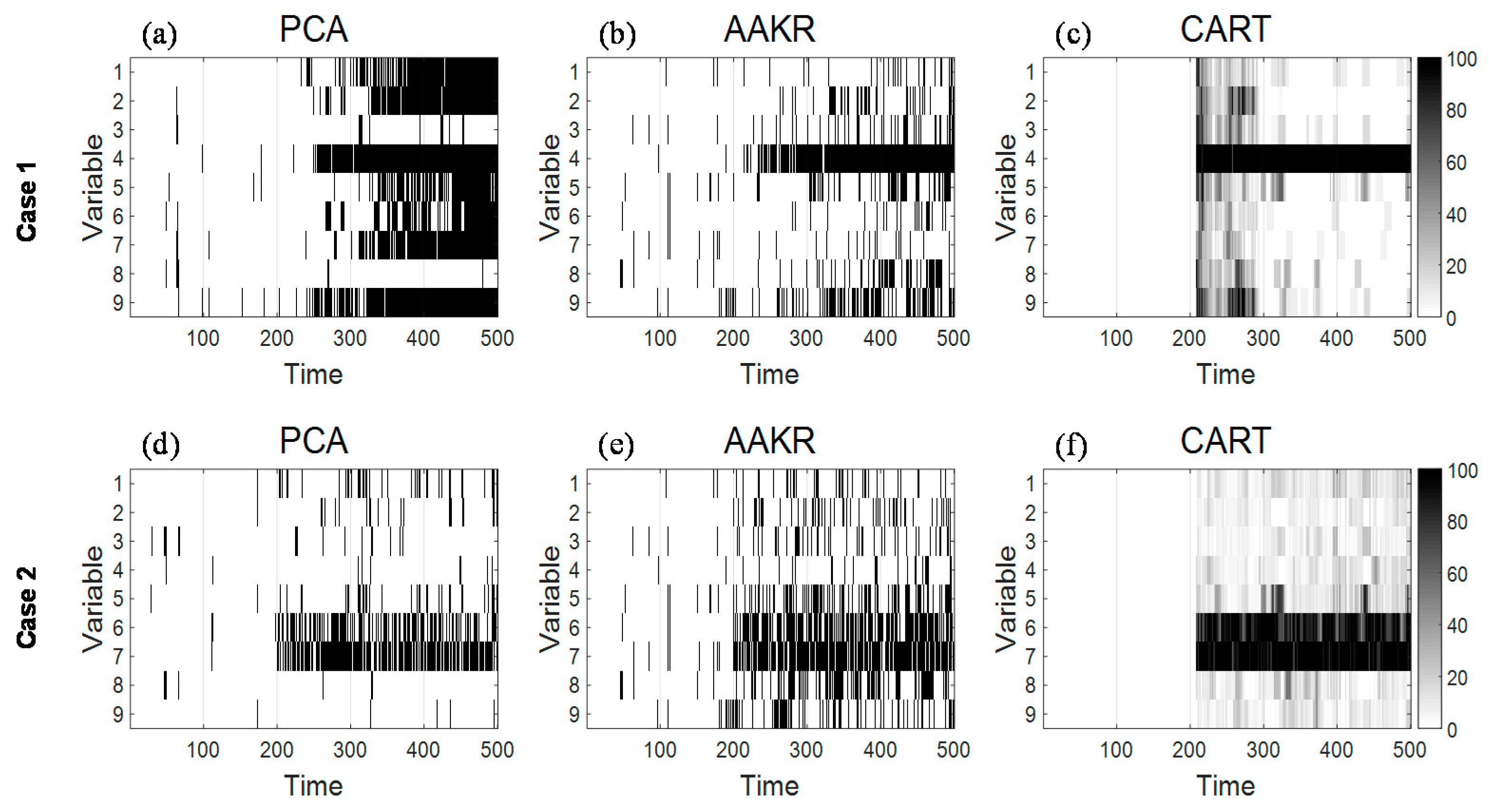
Figure 9 summarizes the fault isolation results obtained by applying comparison methods (PCA- and AAKR-based contribution plots) and Method 2 into Cases 1 and 2. In Figure 9a,d, Q and T² statistics-based contribution plots are used for fault isolation, respectively. First, let us look into the isolation results related with Case 1. As can be seen from Figure 9a, contribution plot for Q statistic suffers from smearing effect; it is observed that severe smearing arises at non-faulty variables x₁, x₂, x₅, x₆, x₇, and x₉. In Figure 9b, contribution values of x₄ start to consistently depart from in-control region at about time t = 230; although the magnitude of the drift fault becomes larger, minor fault smearing in some normal variables (i.e., x₂, x₅, x₈, x₉) is observed in Figure 9b. In the case of Method 2, normal variables as well as faulty variable x₄ have relatively high importance values in the early stage of the drift fault (from about time t = 210 to 290); in the time period from t = 300 to the end, we can confirm that Method 2 can isolate faulty variable x₄ more precisely than comparison methods.

In Case 2, contribution plot for T² statistic of PCA isolates faulty variables x₆ and x₇ more clearly than that of AAKR; but contribution values for x₆ deviate from threshold values insignificantly. In Figure 9e, it is observed that fault smearing in normal variables x₅, x₈, and x₉ has happened. It is apparent from Figure 9d,e,f that Method 2 achieves clearer isolation results than comparison methods.

Next, let us take a look at the isolation results based on Method 1, which are presented in Figure 10. In Cases 1 and 2, the values of $t_{\mathrm{end}}^{\mathrm{fault}}$ are set as 500 and 400, respectively, and the value of $t_{\mathrm{start}}^{\mathrm{fault}}$ is set as 301 in both cases; here, 2000 normal samples (also used to train PCA and AAKR) constitute the normal data matrix X^normal. As presented in Figure 10a, importance value of main steam temperature (x₄) is nearly 100, and the values of the others are less than 30; as a result, we can decide x₄ as major variable for discriminating normal and faulty samples of Case 1 in the original input space. In Figure 10b, it can be observed that the variable importance values of furnace pressure (x₆) and drum level (x₇) are extremely higher than those of others.

Figure 11 shows the constructed tree from which the importance values in Figure 10b are extracted and the corresponding scatter plot of normal and faulty samples (from $t_{\mathrm{start}}^{\mathrm{fault}}$ = 301 to $t_{\mathrm{end}}^{\mathrm{fault}}$ = 400). Only faulty variables x₆ and x₇ are used as split variables in Figure 11a; the other variables do not appear in the final tree. As shown in Figure 11b, the classification tree based on nonparametric CART algorithm can successfully define decision boundaries for separating normal and faulty samples.

4.3.2. Failure Data Due to Waterwall Tube Leakage

In this subsection, we provide the results of applying Methods 1 and 2 to failure data (also investigated in [5,11]) due to waterwall tube leakage, which is gathered from the target boiler in Figure 7. Failure from one or more tubes in the boiler can be detected by sound and either by an increase in the make-up water requirement (indicating a failure of the water-carrying tubes) or by an increased draft in the superheater or reheater areas (due to failure of the superheater or reheater tubes) [38]. The boiler tubes can be influenced by several damage processes such as inside scaling, waterside corrosion and cracking, fireside corrosion and/or erosion, stress rupture due to overheat and creep, vibration-induced and thermal fatigue cracking, and defective welds [42]. Tube leakage from a pin-hole might be tolerated because of an adequate margin of feedwater and the leakage can be corrected after suitable scheduled maintenance [43]. However, if the boiler is continuously operated with the leakage, much of the pressurized fluid will eventually leak and cause severe damage to neighboring tubes. Tube leakage of boiler, superheater and reheater could result in a serious efficiency decline.

Target failure dataset consists of 4273 training and 1054 test samples, respectively; sampling interval is equal to 5 min, and monitored variables are same as those listed in Table 1. The matrix X^training is composed of the training samples and they should be collected from the target boiler under normal operating conditions. The tube leakage occurred at 911th test sample, and after about 12 hours, unplanned shutdown procedures were initiated. 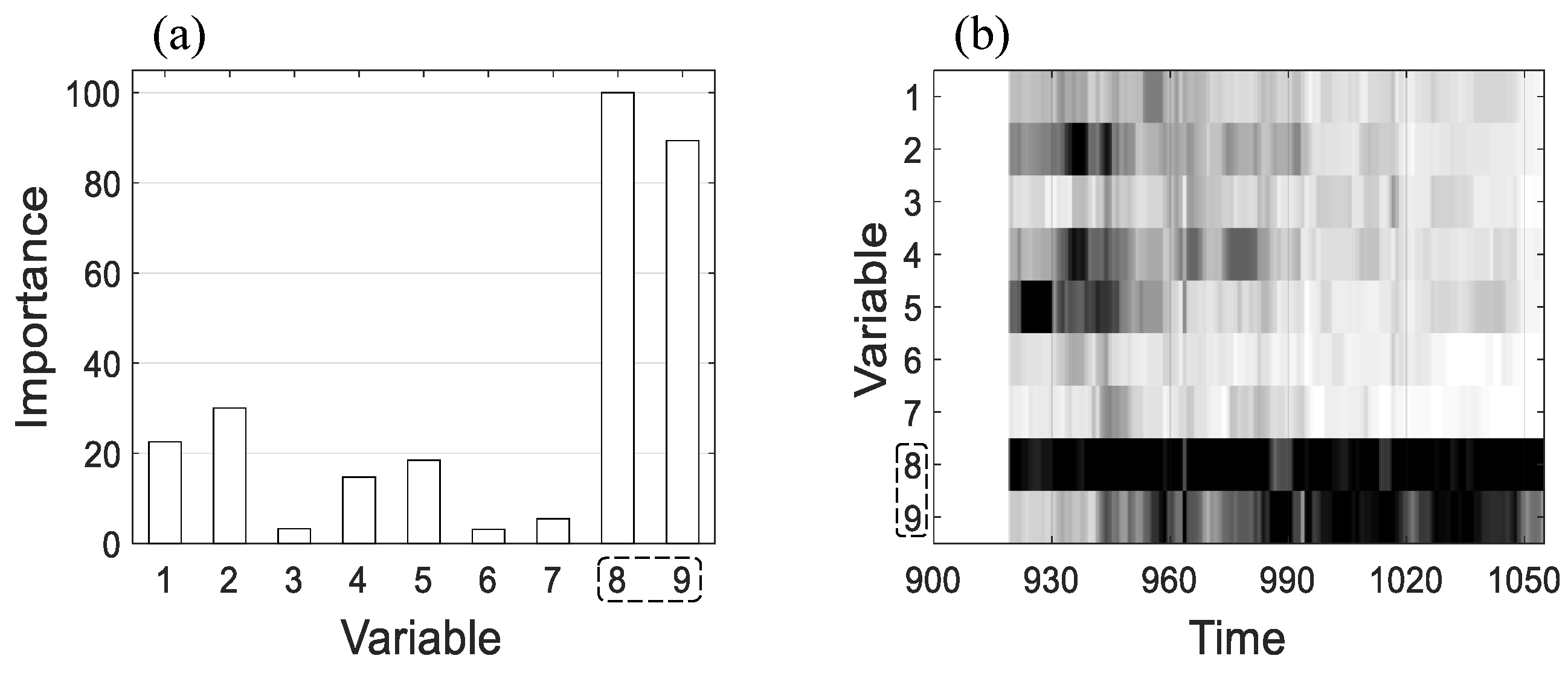Figure 12 shows the fault isolation results for the failure dataset based on Methods 1 and 2; here, $t_{\mathrm{start}}^{\mathrm{fault}}$ and $t_{\mathrm{end}}^{\mathrm{fault}}$ are set as 951 and 1050, respectively. As can be seen from Figure 12a, importance values of condenser make-up flow (x₈) and feedwater flow (x₉) are larger than 80 in the time interval (from t = 951 to t = 1050); those of others in the interval are smaller than 40. In Figure 12b, normal variables such as x₂, x₄, and x₅ exhibit high importance values temporarily at the beginning of the leakage; as the strength of leakage becomes larger, faulty variables x₈ and x₉ are precisely isolated. 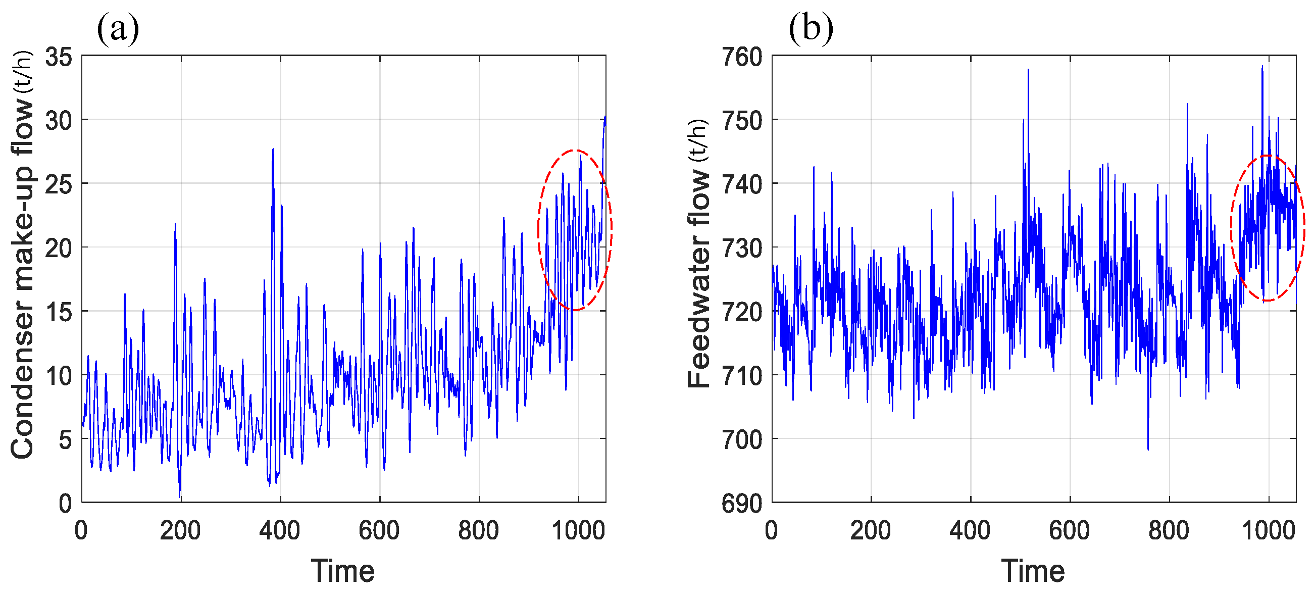Figure 13 describes the trajectories of the faulty variables (x₈ and x₉) in the test period; it can be observed that condenser make-up flow and feedwater flow start to rise sharply at the time t = 911.

4.4. Discussion

In this subsection, we summarize the strengths of the proposed fault isolation method, which are confirmed from the experimental results in Section 4.1, Section 4.2 and Section 4.3. The main strength of the proposed method is that it does not suffer from smearing effect. As shown in Figure 2, Figure 4, and Figure 9, PCA- and AAKR-based contribution plots are troubled with smearing effect; in contrast, the proposed isolation method (i.e., Method 2) can clearly locate faults without the smearing as the fault magnitude becomes larger. In PCA, the contribution values are obtained through projecting query samples in the original space onto a reduced latent space; latent variables are linear combinations of all original variables. Therefore, contribution values of non-faulty variables are also influenced by faulty variables. In AAKR, each component of predicted vectors is a function of both non-faulty and faulty variables; contribution analysis based on the predicted vectors also suffers from fault smearing. The proposed method locates faults by selecting original input variables with higher explanatory powers to discriminate normal and faulty samples. In other words, the proposed method does not suffer from smearing effect because it is based on CART classifiers with decision boundaries only in the original input space. The second strength is that, as described in Figure 4 and Figure 5, the proposed method can properly identify faulty variables of nonlinear process. PCA with the assumption of process linearity is unsuitable for fault detection and isolation of nonlinear processes. As shown in Figure 4, although fault isolation with nonparametric AAKR is troubled with fault smearing, the proposed method can accurately identify faulty variables of the nonlinear process. Except for the strengths mentioned above, the proposed method does not require historical faulty dataset and any prior knowledge and experience.

5. Conclusions

In complex and nonlinear industrial processes, data-driven fault detection and isolation for process monitoring has become more important than ever before; compared with fault detection, fault isolation methods have not been studied very much. In this paper, we proposed a fault isolation method for a drum-type steam boiler via CART-based variable ranking. Method 1 is intended to identify faulty variables in entire fault regions, and it is proper for post analysis of occurring faults offline. In Method 2, fault isolation is carried out through time window sliding; Method 2 is suitable for monitoring fault evolution and propagation. To validate the fault isolation performance, the proposed method and comparison methods were applied to two benchmark problems and 250 MW drum-type steam boiler. The experimental results showed that the proposed method can locate faults more clearly than comparison methods without being affected by smearing effect. The proposed method, based on nonparametric CART, can properly deal with nonlinear processes, and can correctly identify faulty variables, even when normal and faulty samples are linearly inseparable from each other.

In future research, we will consider the following three topics. The first topic is to verify the performance of proposed method for time-varying processes. For example, since the process equipment is gradually degraded over time, it usually shows time-varying behaviors. If components of the matrix X^normal (see Figure 1) are updated with the latest normal samples at every moment, the proposed method may take the time-varying characteristics of target systems into consideration for fault isolation. Second, we will also perform comparative studies between the proposed method and recently developed methods in [27,28,44,45]; this will further ensure the validity of the proposed method. Lastly, to improve the isolation performance, we will develop variable ranking methods with consideration for structural properties (described in [46]) of binary decision trees.