Article

Reliability Assessment of Power Systems with Photovoltaic Power Stations Based on Intelligent State Space Reduction and Pseudo-Sequential Monte Carlo Simulation

School of Electrical and Electronic Engineering, North China Electric Power University, Beijing 102206, China
*
Author to whom correspondence should be addressed.
Energies 2018, 11(6), 1431; https://doi.org/10.3390/en11061431
Submission received: 8 April 2018 / Revised: 9 May 2018 / Accepted: 22 May 2018 / Published: 3 June 2018
(This article belongs to the Special Issue Distribution Power Systems and Power Quality)

Abstract

:
As the number and capacity of photovoltaic (PV) power stations increase, it is of great significance to evaluate the PV-connected power systems in an effective, reasonable, and quick way. In order to overcome the challenge of PV’s time-sequential characteristic and improve upon the computational efficiency, this paper presents a new methodology to evaluate the reliability of the power system with photovoltaic power stations, which combines intelligent state space reduction and a pseudo-sequential Monte Carlo simulation (PMCS). First, a non-aggregate Markov model of photovoltaic output is established, which effectively retains some time-sequential representation of the PV output. Then, the differential evolution algorithm (DE) is introduced into the sampling stage of PMCS to carry out an intelligent state space reduction (ISSR). By using the DE algorithm, success states are searched out and removed, thus the state space is reduced and formed with a high density of loss-of-load. Hence, unnecessary samplings are avoided, which optimizes the PMCS sampling mechanism and improves the computational efficiency. Finally, the proposed method is tested in the modified IEEE RTS-79 system. The results indicate that this new method has a better computational efficiency than the time-sequential Monte Carlo simulation method (TMCS) and pure PMCS. In addition, the effectiveness and feasibility of this method are also verified.

1. Introduction

As photovoltaic (PV) power generation is one of the most important renewable energies, grid-connected photovoltaic power stations have aroused attention around the world and have been developed and utilized rapidly. With the increasing penetration of PV in power systems, the power system faces the impact of random fluctuations of PV output. Therefore, it is necessary to make accurate assessments of the reliability of PV-connected power systems. The reliability indices are of great significance for the power system to plan its expansion, arrange power generation, and energy trading [1,2,3]. However, the time-sequential characteristics and fluctuations of PV output will increase the computational amount in any reliability assessment. Therefore, it is particularly important to evaluate the reliability of PV-connected power systems in an effective, reasonable, and quick way.
At present, the reliability assessment methods for power systems are generally divided into the analytical method and the Monte Carlo simulation (MCS) method. MCS can get rid of the constraints of the system scale and is particularly suitable for large-scale composite power systems [4,5]. In addition, MCS includes two types: time-sequential MCS and non-sequential MCS. However, the characteristics of PV makes the reliability assessment work face greater challenges. On one hand, considering the model of a PV power plant in a simulation method, the computational amount will become extremely complicated when a PV has a large number of states. On the other hand, due to the continuous development of modern power systems and the increasing improved reliability level of the system as well as its components, the computational efficiency of MCS is gradually reduced.
In order to obtain reliability indices with high efficiency, a lot of research has been conducted at home and abroad. Common methods include the stratified uniform sampling method, the importance sampling method, and state space reduction. In the stratified sampling method [6,7], the sampled space is divided into several sub-spaces, sampled separately, and then the indices of these sub-spaces are integrated. Thus, the variance is reduced by reasonably allocating the proportion of the sampling results in each sub-space. In [8], an important sampling method based on the optimal multiplier is proposed, and the optimal multiplier is continuously reconstructed by the component state each time the system failure occurs. At last, the construction of the importance distribution function is completed. In [9], the cross entropy algorithm is used in importance sampling, and the optimal probability model of system components is established, based on the cross entropy algorithm, to reduce the variance coefficient of the sample space. It is worth mentioning that state space reduction is an effective methodology by which most of the success states can be reduced out from the original state space by a certain sampling mechanism. And the remaining state space with a higher density of loss-of-load states allows the MCS to obtain more loss-of-load states in sampling, which in turn, speed up the convergence of the variance coefficient. Based on state decoupling, Mitra and Singh et al. proposed a state space reduction method in 1996, which achieved the reduction of the state space [10,11,12]. In recent years, on this basis, scholars at home and abroad have fully exploited the fast and random search ability of this intelligent algorithm. Therefore, the method of the Intelligent State Space Reduction (ISSR) is formed systematically. In [13,14,15], the genetic algorithm and the binary particle swarm both are used in state space reduction to speed up the convergence of MCS. In [15], the performance comparison of the intelligent state space reduction is carried out under different heuristic algorithms. In the comparison, not only are the proposed genetic algorithm and binary particle swarm algorithm considered, but the mutex binary particle swarm and binary particle swarm optimization are also involved.
However, the methods mentioned above are all applied to the framework of the non-sequential Monte Carlo method. Taking into account that a large scale of renewable energies and other components connect to the grid, the non-sequential Monte Carlo method is no longer applicable due to the time sequential properties of the components and correlation with the adjacent system states cannot be depicted. Therefore, the improved sequential Monte Carlo method will have a wider application prospect. As has been confirmed, the parallel computation technique and pseudo-sequential Monte Carlo simulation can effectively improve the computational efficiency of TMCS [16]. The parallel computation technique is the parallel computation and information interaction between multiple computers, analyzing and calculating the power flow for the system states at each time section. By using this technique, the computational time is reduced and in the meantime it depends on the computer hardware equipment. The pseudo-sequential Monte Carlo simulation (PMCS) [17] is the combination of the sequential and non-sequential Monte Carlo method. To be specific, the loss-of-load states are sampled randomly by the non-sequential Monte Carlo method, followed by constructing the sub-sequences of the loss-of-load states via the time-sequential Monte Carlo method. Only partial states need to be analyzed for the time-sequential information, which improves the computational efficiency and is thus called a “pseudo-sequence”. Although the pseudo-sequential MCS can improve computational efficiency, it is still at a distinct disadvantage when compared with non-sequential MCS. In [18], the state transition technique is applied to the pseudo-sequential simulation and this technique is used to speed up the formation of the sub-sequence of the loss-of-load states. However, it is shown that the time-consumption of the pseudo-sequential simulations is mainly due to a large number of ineffective states (success state) that are sampled and evaluated in the non-sequential process [19]. The adoption of a more advanced state sampling mechanism will further improve the computational efficiency of PMCS.
In view of all the above considerations, this paper proposes a kind of PMCS method based on an ISSR. First, a non-aggregated Markov model of photovoltaic power generation is built to make it appropriate to the process of a pseudo-sequential simulation. Secondly, the differential evolution algorithm is introduced in the process of intelligent state space reduction, so the success states can be quickly sought and the set of success states can be established. By this way, the sampling mechanism is optimized by ISSR, which greatly increases the probability of sampling loss-of-load states and reduces the amount of work in the states’ evaluation. Therefore, the improvement of the existing PMCS is realized.

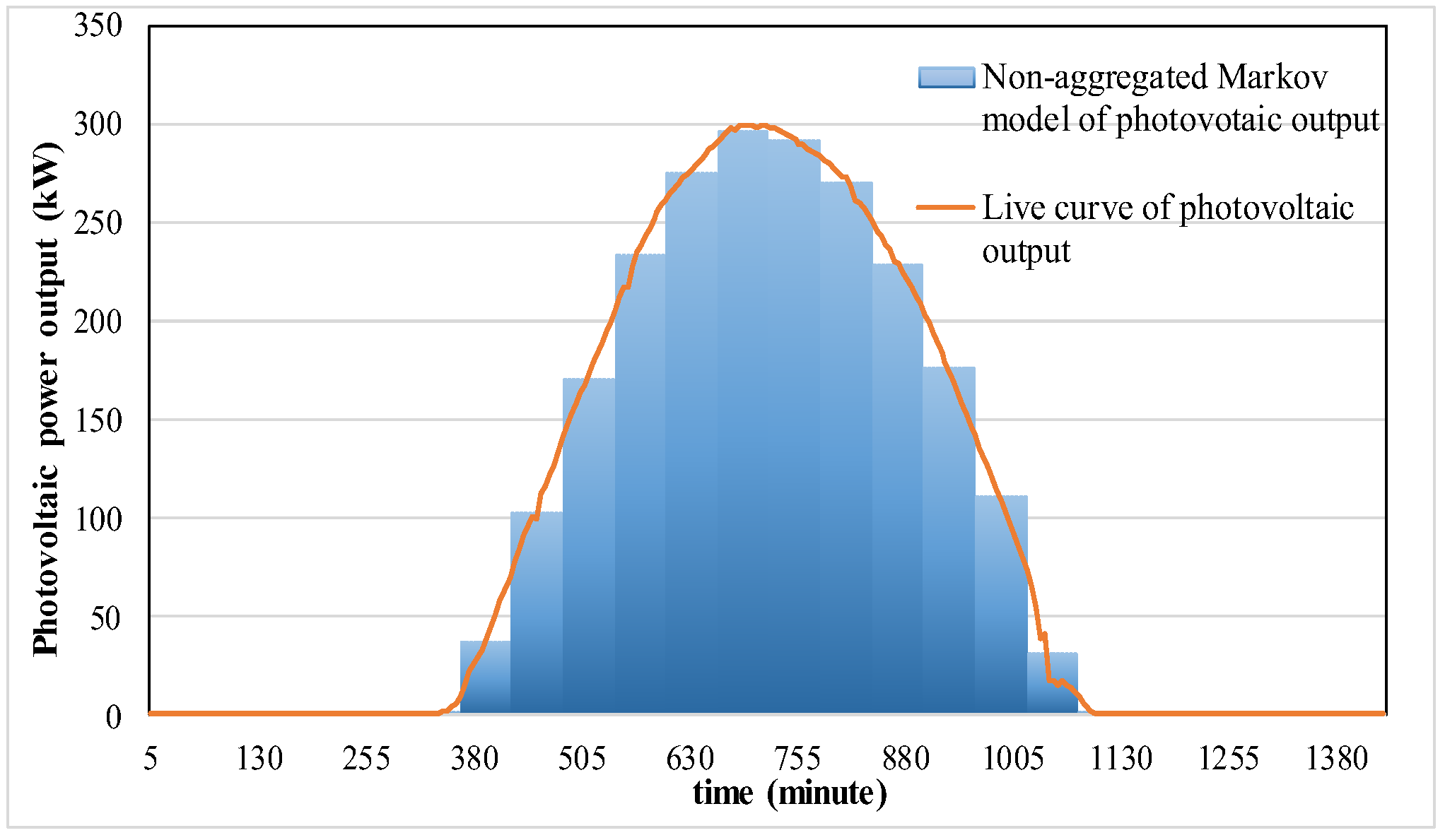
2. Non-Aggregate Markov Model of Photovoltaic Output

As a result of the photovoltaic power out being time varying, the best option to assess the reliability of a PV-connected power system is by using the time-sequential Monte Carlo simulation. However, a huge amount of CPU time is needed for such a detailed simulation, which can make the evaluation unfeasible for large and complex systems. Considering this difficulty, in order to retain the time-sequential characteristics of PV output as much as possible, a non-aggregate Markov model of the photovoltaic power generation is proposed here, which can make it better applied to the evaluation method that is going to be proposed in the following sections.
As is shown in Figure 1, in the photovoltaic output model, the total hours of a year T is divided into Q intervals with the same length ∆T. For the interval i, the photovoltaic output Pi takes the mean value of statistical data during the interval i. Then, according to the time sequence of the PV output curve, all the PV output states are linked in chronological order. In this model, a constant transition rate of λ = 1 Δ T between two connected states is adopted. Thus, a non-aggregate Markov model of photovoltaic power generation is formed.

3. Power System Reliability Evaluation Based on Pseudo-Sequential Monte Carlo Simulation (PMCS)

3.1. Basic Theory of PMCS

PMCS is a combination of the sequential Monte Carlo simulation (TMCS) and the non-sequential Monte Carlo simulation, which also maintains the flexibility and accuracy of TMCS while speeding up the system reliability evaluation. Compared with the TMCS, PMCS only takes into account the sequential information of the sub-sequences of the loss-of-load states, which contributes to the reliability indices in the simulation process. In PMCS, the system states are randomly sampled based on non-sequential MCS. If the sampled state is in the loss-of-load state section, then mark this section as the starting point. Based on the state transition equation of the loss-of-load states set, the time duration is respectively extended backward and forward from the starting point until to a certain success system state is achieved, thus forming the subsequence of the loss-of-load state.
The subsequences of the loss-of-load states are formed via forward and backward simulation, which is shown in Figure 2, and the procedures are as follows:
(1)
Forward time-sequential simulation: starting from the selected loss-of-load state Xs, the state transition process continuously goes on until it reaches a success state. The probability for the state transition from Xs to Xt is expressed as:
P s t = f s t f s o u t = [ P ( X s ) λ s t ] / [ P ( X s ) i = 1 M s λ s i ]
where fst is the frequency of system state Xs transferring to Xt; fsout is the frequency of departure from state Xs; P(Xs) is the occurrence probability of the state Xs, λst is the transition rate of the component whose state changes during the transferring process from Xs to Xt; Ms is the number of states which the system can turn into after leaving the state Xs.
(2)
The time-sequential backward simulation: starting from the selected loss-of-load state Xs, continue the state transition process of backwards until success state is found. The probability of the state transition from Xt to Xs is:
P r s = f r s f s i n = [ P ( X r ) λ r s ] / [ i = 1 M r P ( X i ) λ i s ]
where frs is the frequency that the system state Xr transferring to Xs; fsin is the frequency of arriving at state Xs; P(Xi)is the occurrence probability of the state Xr; λis is the transition rate of the state changing component whose state changes during the transferring process from Xi to Xs; Mr is the number of states that the system can arrive at the state Xs.
For the failure subsequence formed by the forward/backward simulation, the total time expectation of the failure duration can be expressed as:
E [ D s ] = i s E [ D i ] ,
where
E [ D i ] = 8760 / [ j λ j ]
where E[Di] is the time expectation of failure duration in the ith system state within the failure subsequence, and λj is the transition rate.

3.2. Computation of PMCS Reliability Indices

During the simulation process of PMCS, only the failure sequences are taken into account. Therefore, in order to decrease the error deviation, it is necessary to force the reliability indices to map back to the original state space. The basic principle of computing the PMCS reliability indices is to convert the reliability indices based on the failure subsequence into those based on the common sampled states. In the PMCS, the expected values of LOLP (Loss of Load Probability) and EENS (Expected energy not supplied) can be expressed as [19]:
E [ H L O L P ] = 1 N i = 1 N H L O L P ( X i ) ,
E [ H E E N S ] = 1 N i = 1 N H E E N S ( X i )
where N is the overall times of non-sequential sampling. HLOLP(Xi) and HEENS(Xi) are the test results of sampled state Xi corresponding to the reliability indices, which are given as follows:
H L O L P ( X i ) = { 1 X i X f 0 X i X f ,
H E E N S ( X i ) = { S j M i P S ( S j ) D ( S j ) S j M i D ( S j ) X i X f 0 X i X f ,
where Mi is the sub-sequence generated from loss-of-load states; PS(·) is the load curtailment of a certain state; D(·) is the duration of a certain state Sj; Xf is the set of loss-of-load states.

4. Pseudo-Sequential Monte Carlo Simulation Based on Intelligent State Space Reduction

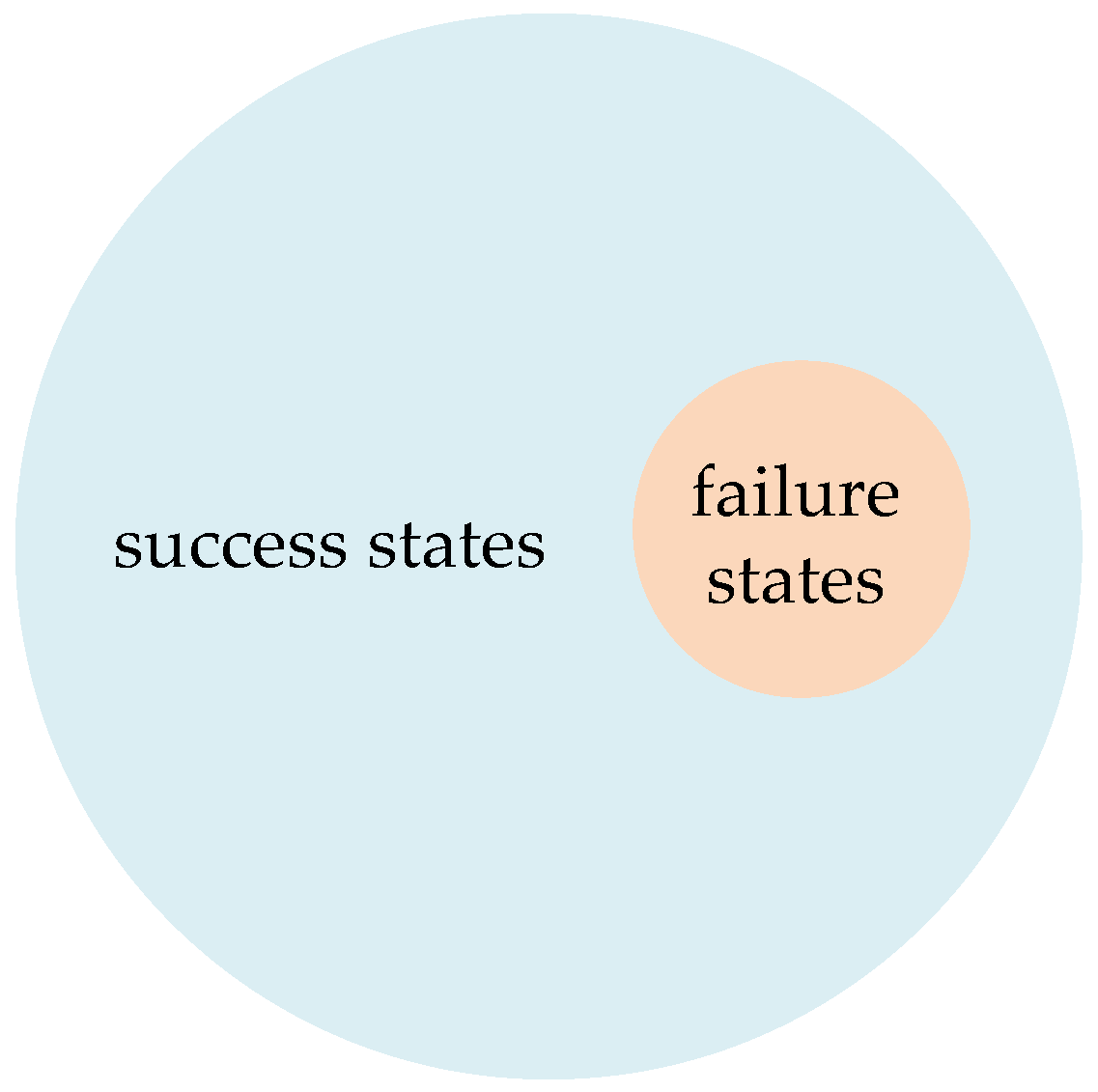
4.1. The Concept of Intelligent State Space Reduction

For the power system, the vast majority of system states are success states, while the loss-of-load states just account for a small proportion (The distribution of the power state space is shown in Figure 3). However, the success states contribute less to the reliability indices calculation, resulting in a large number of invalid samples during the sampling process.
The ISSR is an effective method to facilitate the sampling of loss-of-load states. The first step is to guide the generation evolution via the intelligent algorithm, and in the process of population generation, the success states are quickly searched and stored in the set of success states. Then the set of success states is moved out of the original overall state space, and as a result of which, due to the remaining state space having a higher density of loss-of-load states, the probability of loss-of-load states to be sampled is greatly increased. With the same convergence accuracy, compared with traditional Monte Carlo sampling, this approach features fewer samples needed and less time-consumption. The sketch of the ISSR is shown in Figure 4.

4.2. The Intelligent State Space Reduction Based on Differential Evolution Algorithm

The differential evolution algorithm is a heuristic random search algorithm based on population differences, attracting much more attention because of its simple principle, less control parameters, and strong robustness. The operation flow of DE is similar to that of other evolution algorithms, including mutation, crossover, and selection. A differential strategy is used for DE’s mutation operation, that is, by using the differential vectors between individuals within a generation to interrupt the individuals, the mutation of individuals can be achieved. DE’s mutation operation effectively utilizes the population distribution to improve the search ability, and in this way, the deficiency of mutation in the Genetic Algorithm is overcome. Therefore, this paper adopts DE to guide the generation evolution, thus completing the rapid search for success states. Let Xi,t denote the individual i (i.e., the system state) in generation t, which is expressed as follows:
X i , t = ( x i , t 1 , x i , t 2 , , x i , t n ) ,   i = 1 , 2 , , M ,
x i , t j = { 0 , s u c c e s s   s t a t e 1 , f a i l u r e   s t a t e j = 1 , 2 , , n ,
where xji,t indicates the state of component j in the ith individual, tth generation. 0 represents success state, 1 represents failure state, n is the number of system components, and M indicates the size of the generation population.
For all individuals in the generation population, it is important to set the appropriate fitness function. In this paper, referring to previous work, the fitness function Fit(k) is defined as follows [13]:
F i t ( k ) = C o p y k × P k × E k ,
where Copyk represents the number of all possible permutations of the system state k, the generator set can be divided into m groups according to its rated capacity, Gj represents the total number of generators in the jth group, and Oj is the total number of normal working generators in the jth group, which can be represented by:
C o p y k = [ G 1 O 1 ] ... [ G j O j ] ... [ G m O m ] ,
where Pk represents the probability that the system state k occurs, which can be represented by:
P k = i = 1 n p i ,
p i = { 1 F O R i , N o r m a l   w o r k i n g   c o m p o n e n t   i F O R i , F a i l e d   c o m p o n e n t   i ,
where: FORi represents the unavailability of component i; Ck represents the total power generation capacity in state k generators set, and Uk represents the actual power generation capacity in state k generators set after the optimal power flow (OPF); Ek is the surplus power supply in state k, which is expressed as:
E k = { C k U k , s u c c e s s   s t a t e s   U k C k , f a i l u r e   s t a t e s   ,
The fitness function will guide the system to increase the total power generation capacity and circuit capacity, which can further facilitate the intelligent search for the success states. The intelligent algorithm aims to search out more success states in a short period of time rather than to solve an optimization problem. Therefore, the stopping criterion of ISSR is supposed to be the number of generations.
The steps for the state space reduction based on DE are as follows:
Step 1: Generate the first generation of population according to the unavailability of individual components, and the fixed size of population is M.
Step 2: Identify each individual in the population and judge whether it is a success state; if so, store the individual in the set of success states.
Step 3: Individual evaluation. The fitness function values for each individual Xi,t are calculated by Equation (11).
Step 4: Mutation operation. For each individual Xi,t in the population, the three mutually different integers r1, r2, r3 ∈ {1, 2, …, M} are randomly generated, and the four numbers r1, r2, r3, and i are required to be different from each other. Since each individual is represented by a binary bit string, the logical operation is adopted instead of the arithmetic operation to ensure that each individual bit string in the evolution generations can only be 0 or 1. As “ ” is used to indicate “exclusive OR” operation, “ ” indicates “and”, and “+” indicates “or”, finally the mutation individual Vi,t is produced according to the Equation (16):
V i , t = X r 1 , t + F ( X r 2 , t X r 3 , t ) ,
where the mutation factor F is a randomly-generated binary bit string.
Step 5: Cross operation. For the mutation individual Vi,t and the target Xi,t in the population, based on Equation (17), the test individual is Ui,t = (u1i,t, u2i,t, …, uni,t). In order to ensure the evolution of the individuals, first of all, make sure that at least one in the Ui,t is attributed by Vi,t and the others are attributed either by the Vi,t or by the Xi,t, which is determined by the crossover probability CR.
u i , t j = { v i , t j , i f   r a n d j C R o r j = j r a n d x i , t j , o t h e r w i s e ,
where randj is an evenly distributed real number randomly chosen between [0,1], and jrand is a random integer of [1, 2, ..., n].
Step 6: Selection operation. The “greedy selection” strategy is adopted in this operation. The test individual Ui,t and the target individual Xi,t are made to compete with each other, and the one with better fitness value is selected as the individual of the generation t + 1.
X i , t + 1 = { U i , t   F i t ( U i , t ) < F i t ( X i , t ) X i , t   F i t ( U i , t ) F i t ( X i , t ) i = 1 , 2 , , M ,
Step 7: Determine if the convergence criteria are met, that is, whether the fixed generations have been reached or not. If not, return to step 2; otherwise, stop the process of intelligent state space reduction.

4.3. The Evaluation Process of the PMCS Based on the Intelligent State Space Reduction

In view of the rare occurrence of loss-of-load events in the power system, it always takes much time to sample and evaluate the loss-of-load states in the non-sequential process of the PMCS. Therefore, in this part, a PMCS method based on ISSR is introduced to improve the probability of sampling the loss-of-load states and accelerate the computational speed. The simulation process can be divided into two parts. The first part is the process of intelligent state space reduction, which establishes the set of success states via ISSR. And the second part comes to the computational process of reliability indices via PMCS. In the computational process, firstly, the system states are randomly sampled by the non-sequential Monte Carlo simulation to search for the loss-of-load states in the reduced state space. For a sampled loss-of-load state, on the one hand, the loss-of-load state subsequence is determined by the forward/backward simulation until arriving at a success state. On the other hand, the point-in-time needs to be randomly sampled, at which point the loss-of-load event occurs. Once it is determined, in the duration of the loss-of-load state subsequence, the power generation of renewable energy can be obtained according to its time-sequential power curve. The flow chart of this algorithm is shown in Figure 5.

5. Case Study

In this paper, the methodology was implemented in a MATLAB platform and all computations were performed on a 64-bit Windows 7 system with an Intel i7-2600 CPU (4 cores at 3.4 GHz), 4 GB RAM. A modified IEEE RTS-79 is taken as the test system, which has a total installed capacity of 3405 MW and a total peak load value of 2850 MW, consisting of 24 nodes, 38 lines, 32 generators, and a compensator. It is assumed that the size M of each generation population is 300, the crossover probability CR is 0.5, and the variation factor F is a randomly generated binary string (the probability for each bit to generate 0 or 1 is equal). At node 16, a PV power station is added, which has a total installed capacity of 150 MW, including 500 PV units with a capacity of 300 kW each. Figure 6 shows the real-time power curve and a non-aggregated Markov model for an individual PV unit in a typical day as well as in a certain region of northwest China. The real-time power curve is obtained from an individual photovoltaic unit in a PV power station, which is located at 34°16′ N, 108°54′ E. The angle of inclination of the photovoltaic modules is 19° southeast and the angle of orientation is 26°. The PV output value used in this paper is taken from the actual output data of the PV rooftop power station on 1 February 2018, and the acquisition step length is 5 min. For the non-aggregated Markov model of PV output, T is 24 h, ∆T is 1h. It can be seen from Figure 6, the non-aggregated Markov model simplifies the live power curve, and meanwhile, it retains some time-sequential characteristic of PV output.

5.1. The Effects of DE on Generation Superiority

The purpose of the ISSR is to search for more success system states, so this paper regards the number of the success states in each generation as the reference criterion to measure the excellence of the population. In the process of reduction, the number of the success states in each generation changes along with the generation, which is as the curve shows below.
Figure 7 indicates that the number of success system states presents an upward trend along with the generations, which proves that the DE has successfully optimized the generations and achieved the generation evolution.

5.2. The Effects of Generations on Computational Efficiency

The pseudo-sequential Monte Carlo simulation based on the ISSR can be generally divided into the process of ISSR and the reliability indices computation. The number of the generations, on the one hand, influences the scale of the individual states to be assessed in the process of ISSR. On the other hand, the density of the loss-of-load states in the reduced state space is also changed, which influences the computational efficiency of the reliability indices. The EENS variance coefficient of 5% is taken as the convergence index, and the computational time is compared and analyzed when the set number of generations is 50, 60, 70, and 80. The computational time change alongside the generations is shown in Table 1.
As it is shown in Table 1, the ISSR time increases linearly along with the increase of generations, while the computational time for the reliability indices decreases. This is because in the process of ISSR it is necessary to evaluate all individual states in the generations by calling OPF. Because the evaluation time spent on each individual is of little difference, as a whole, the spending time shows a linear increase. The more the generations, the larger the scale of the success states set will be, and the higher the density of the loss-of-load states in the reduced state space will be. Therefore, the variance convergence becomes faster with more generations, thus shortening the computational time of the reliability indices. When a generation increases from 60 to 70, the computational time of the reliability indices decreases the most. However, from 70 to 80, the decrease becomes the smallest. This is mainly because during the multiplying process from 60 to 70 generations, some success states newly emerge with larger probability. In this case, the set of success states includes the vast majority of the success states. Thus, the density of the loss-of-load states in the reduced state space increases greatly and the computational time decreases dramatically. However, during the multiplying process from 70 to 80, the generations have almost completely evolved. The diversity of generations and the scale of the success states have not improved so greatly. Therefore, compared with 70 generations, the decrease of the computational time is not obvious. When it is 70 generations, the total time is 3142.54 s, which is the optimum process of state space reduction and computation of the reliability indices.

5.3. Algorithm Comparison

In this section, the EENS variance coefficient of 5% is taken as the convergence index, and the proposed method is compared with traditional PMCS and TMCS. In the proposed method, with 70 chosen as the number of generations, the process of state space reduction as well as the computation of reliability indices is in the optimum. The results of the computation are shown in Table 2. According to (5) and (6), for PMCS and the new algorithm, reliability indices should be updated once after each time of the non-sequential sampling process. With LOLP and EENS obtained via TMCS made as the benchmark, the convergence processes of LOLP and EENS, as well as their variance change curves, are shown in Figure 8 and Figure 9.
Figure 8 and Figure 9 indicate that the LOLP and EENS indices calculated by the PMCS and the new algorithm are almost equal to that calculated by the TMCS, which verifies the effective feasibility of PMCS and the new algorithm proposed in this paper. Table 2 shows that, the total computational time of the new algorithm is 3142.54 s, including the time of 2038.17 s spent for the computation of reliability indices and the time of 1104.37 s spent for the ISSR (see Table 1). When compared with the TMCS and PMCS, the computational efficiency of the new algorithm increases by 13.08 times and 1.74 times respectively. The PMCS only considers the time-sequential information of the loss-of-load subsequence, so its computational efficiency is higher than that of TMCS. As for the new algorithm, the state space with a high density of loss-of-load is established by ISSR, which greatly reduces the computational time of reliability indices and the total computation efficiency has been improved.
The subsequent work further verifies the improvement of ISSR to PMCS in the new algorithm. In the following analysis, T indicates the total number of non-sequential random samplings in PMCS, and D indicates the number of samplings in which the sampled states belong to the set of success states. For the remaining T-D samplings, the density of loss-of-load states is much higher via ISSR, that is, the majority of the states are loss-of-load states. By contrast, the traditional PMCS tends to a much lower density of loss-of-load states, that is, most of them are the success states. Here the number of non-sequential samplings of loss-of-load states is represented by S, and so the density of the loss-of-load states is represented as S/(T-D). The comparing results are shown in Table 3.
As can be seen from Table 3, in the random sampling process via traditional PMCS, D equals 0. This is so because the set of success states is not established, and thus it is necessary to evaluate all the sampled states. In this case, its density of the loss-of-load states is 4.04%. But in the new algorithm, there is no need to evaluate the states in the set of success states by calling OPF. The results of LOLP and EENS both are 0, the total number of times for the non-sequential sampling is 30,964, and 28,134 of them are for the success states. Therefore in the new algorithm, only 2830 samplings are used for the state evaluation, hence the computational time for evaluating success states is greatly shortened. In the new algorithm, the density of loss-of-load events in the reduced state space is up to 43.22%, which is more than ten times that of using a traditional PMCS. On the basis of PMCS, the introduction of ISSR effectively optimizes the sampling mechanism of non-sequential simulation, further improving the efficiency of sampling the loss-of-load states and accelerating the computation speed.
In the above study, the modified IEEE RTS-79 system is a calculation example mainly used to verify the computational efficiency of this algorithm. In practice, this study has been supported by the practical project and is successfully applied to the electric power system of Zhejiang province in China. According to the original data provided by Zhejiang Electric Power Company, Zhejiang’s 500 kV and main 220 kV grids have a total installed capacity of 190,684 MW and a total peak load value of 24,732 MW, consisting of 126 nodes, 85 load points, 197 lines, and 84 generators. And the system spare capacity is 1852 MW. This paper uses the algorithm to evaluate and analyze the reliability of the actual system. Table 4 shows the reliability indices obtained as well as the computation time via the different algorithms.
From Table 4, it can be seen that the new proposed algorithm has significant advantages in the reliability evaluation of practical complex systems and its computational efficiency is much higher than the TMCS and PMCS. Therefore, the proposed method has achieved important application value.

6. Conclusions

This paper proposes a fast reliability evaluation method based on the pseudo-sequential Monte Carlo simulation and intelligent state space reduction, and this proposal is tested in the modified IEEE RTS-79 system. The following conclusions are obtained: (1) Compared with the TMCS and traditional PMCS in reliability indices calculation, the proposed algorithm is performed with higher precision and computational efficiency; (2) The ISSR technique optimizes the traditional PMCS sampling mechanism to a large extent, reducing the times of invalid states sampling. But in the state evaluation process, OPF is still adopted for computation. If the state space can be directly divided by artificial intelligence technology, such as in support vector machines or neural networks, the speed of the reliability evaluation will be further accelerated; (3) The computational time decreases with the increase of the number of normal states reduced, while the computational time for state reduction increases. Thus, as for the use of ISSR, future research will focus on how to reasonably choose the optimal level of state space reduction and harmonize the contradiction between the pruning time and simulation time.

Author Contributions

Conceptualization, D.G. and Y.X.; Methodology, R.C.; Software, Z.W.; Validation, D.G., Y.X. and R.C.; Formal Analysis, D.G.; Investigation, Y.X.; Resources, Y.L.; Data Curation, Y.X.; Writing-Review & Editing, Y.X.; Funding Acquisition, W.L.

Acknowledgments

This work has received funding from the National Key R&D Program of China (2017YFB0903100). The National Key R&D Program of China covered the cost to publish in open access.

Conflicts of Interest

The authors declare no conflict of interest.

References

  1. Mosadeghy, M.; Yan, R.; Saha, T.K. Impact of PV penetration level on the capacity value of South Australian wind farms. Renew. Energy 2016, 85, 1135–1142. [Google Scholar] [CrossRef]
  2. Zhang, P.; Wang, Y.; Xiao, W.; Li, W. Reliability Evaluation of Grid-Connected Photovoltaic Power Systems. IEEE Trans. Sustain. Energy 2012, 3, 379–389. [Google Scholar] [CrossRef]
  3. Zhou, P.; Jin, R.Y.; Fan, L.W. Reliability and economic evaluation of power system with renewables: A review. Renew. Sustain. Energy Rev. 2016, 58, 537–547. [Google Scholar] [CrossRef]
  4. Da Silva, A.M.L.; de Resende, L.C.; da Fonseca Manso, L.A.; Miranda, V. Composite Reliability Assessment Based on Monte Carlo Simulation and Artificial Neural Networks. IEEE Trans. Power Syst. 2007, 22, 1202–1209. [Google Scholar] [CrossRef]
  5. Bakkiyaraj, R.A.; Kumarappan, N. Optimal reliability planning for a composite electric power system based on Monte Carlo simulation using particle swarm optimization. Int. J. Electr. Power Energy Syst. 2013, 47, 109–116. [Google Scholar] [CrossRef]
  6. Alban, A.; Darji, H.A.; Imamura, A.; Nakayama, M.K. Efficient Monte Carlo Methods for Estimating Failure Probabilities. Reliab. Eng. Syst. Saf. 2017, 165, 376–394. [Google Scholar] [CrossRef]
  7. Nanou, S.I.; Tzortzopoulos, O.D.; Papathanassiou, S.A. Evaluation of an enhanced power dispatch control scheme for multi-terminal HVDC grids using Monte-Carlo simulation. Electr. Power Syst. Res. 2016, 140, 925–932. [Google Scholar] [CrossRef]
  8. Gubbala, N.; Singh, C. Models and considerations for parallel implementation of Monte Carlo simulation methods for power system reliability evaluation. IEEE Trans. Power Syst. 1995, 10, 779–787. [Google Scholar] [CrossRef]
  9. Sadeghi, M.; Kalantar, M. Multi types DG expansion dynamic planning in distribution system under stochastic conditions using Covariance Matrix Adaptation Evolutionary Strategy and Monte-Carlo simulation. Energy Convers. Manag. 2014, 87, 455–471. [Google Scholar] [CrossRef]
  10. Mitra, J.; Singh, C. Incorporating the DC load flow model in the decomposition-simulation method of multi-area reliability evaluation. IEEE Trans. Power Syst. 1996, 11, 1245–1254. [Google Scholar] [CrossRef]
  11. Singh, C.; Mitra, J. Composite system reliability evaluation using state space pruning. IEEE Trans. Power Syst. 2002, 12, 471–479. [Google Scholar] [CrossRef]
  12. Mitra, J.; Singh, C. Pruning and simulation for determination of frequency and duration indices of composite power systems. IEEE Trans. Power Syst. 1999, 14, 899–905. [Google Scholar] [CrossRef]
  13. Green, R.C.; Wang, L.; Singh, C. State space pruning for power system reliability evaluation using genetic algorithms. In Proceedings of the 2010 IEEE Power and Energy Society General Meeting, Providence, RI, USA, 25–29 July 2010; pp. 1–6. [Google Scholar]
  14. Green, R.C.; Wang, L.; Alam, M.; Singh, C. State space pruning for reliability evaluation using binary particle swarm optimization. In Proceedings of the 2011 IEEE Power Systems Conference and Exposition, Phoenix, AZ, USA, 20–23 March 2011; pp. 1–7. [Google Scholar]
  15. Green, R.C.; Wang, L.; Wang, Z.; Alam, M.; Singh, C. Power system reliability assessment using intelligent state space pruning techniques: A comparative study. In Proceedings of the 2010 IEEE International Conference on Power System Technology, Hangzhou, China, 24–28 October 2010; pp. 1–8. [Google Scholar]
  16. Kadhem, A.A.; Wahab, N.I.A.; Aris, I.; Jasni, J.; Abdalla, A.N. Computational techniques for assessing the reliability and sustainability of electrical power systems: A review. Renew. Sustain. Energy Rev. 2017, 80, 1175–1186. [Google Scholar] [CrossRef]
  17. Jco, M.; Pereira, M.V.F.; Da Silva, A.L. Evaluation of reliability worth in composite systems based on pseudo-sequential Monte Carlo simulation. IEEE Trans. Power Syst. 1994, 9, 1318–1326. [Google Scholar]
  18. Mello, J.C.O.; Da Silva, A.L.; Pereira, M.V.F. Efficient loss-of-load cost evaluation by combined pseudo-sequential and state transition simulation. IET Proc. Gen. Trans. Distrib. 1997, 8, 147–154. [Google Scholar] [CrossRef]
  19. Zhang, P.; Li, W.; Li, S.; Wang, Y.; Xiao, W. Reliability assessment of photovoltaic power systems: Review of current status and future perspectives. Appl. Energy 2013, 104, 822–833. [Google Scholar] [CrossRef]
Figure 1. Non-aggregate Markov model of photovoltaic output.
Energies 11 01431 g001
Figure 2. The schematic diagram of forward and backward method used in pseudo-sequential Monte Carlo simulation (PMCS).
Energies 11 01431 g002
Figure 3. The constituents of the system state space.
Energies 11 01431 g003
Figure 4. The schematic diagram of Intelligent State Space Reduction (ISSR) algorithm.
Energies 11 01431 g004
Figure 5. The reliability evaluation process by using PMCS based on the ISSR.
Energies 11 01431 g005
Figure 6. The actual power curve and non-aggregate Markov model of photovoltaic power output.
Energies 11 01431 g006
Figure 7. The trend graph that the number of success states change along with the generation.
Energies 11 01431 g007
Figure 8. Convergence process of the Loss of Load Probability (LOLP) index in different algorithms.
Energies 11 01431 g008
Figure 9. Convergence process of the expected energy not supplied (EENS) index in different algorithms.
Energies 11 01431 g009
Table 1. The computational time under different generation numbers.
Generation Number50607080
ISSR time/s795.22952.531104.41259.2
computation time/s3760.33179.72038.21968.4
Total time/s4555.64132.23142.53227.6
Table 2. Comparison of indices with different algorithms.
AlgorithmLOLPEENS/MWhComputation Time/s
TMCS0.04005.550141,107
PMCS0.04055.52075481.0
New algorithm0.03955.59672038.2
Table 3. Comparison of sampling amounts with traditional PMCS and the ISSR-based PMCS.
ContentTSDT-DS/(T-D)
PMCS66,9132707066,9134.04%
New algorithm30,964122328,134283043.43%
Table 4. The reliability indices of practical system obtained via different algorithms.
AlgorithmLOLPEENS(MWh/Year)Computation Time/s
TMCS0.021320,9927 h 43 min
PMCS0.021821,1404 h 18 min
New algorithm0.021621,3852 h 24 min

