Computational Intelligence Techniques Applied to the Day Ahead PV Output Power Forecast: PHANN, SNO and Mixed


Dipartimento di Energia, Politecnico di Milano, Via Lambruschini 4, 20156 Milano, Italy
*
Authors to whom correspondence should be addressed.
Energies 2018, 11(6), 1487; https://doi.org/10.3390/en11061487
Submission received: 29 April 2018
/
Revised: 1 June 2018
/
Accepted: 4 June 2018
/
Published: 7 June 2018
(This article belongs to the Special Issue Solar and Wind Energy Forecasting)
Abstract
:An accurate forecast of the exploitable energy from Renewable Energy Sources is extremely important for the stability issues of the electric grid and the reliability of the bidding markets. This paper presents a comparison among different forecasting methods of the photovoltaic output power introducing a new method that mixes some peculiarities of the others: the Physical Hybrid Artificial Neural Network and the five parameters model estimated by the Social Network Optimization. In particular, the day-ahead forecasts evaluated against real data measured for two years in an existing photovoltaic plant located in Milan, Italy, are compared by means both new and the most common error indicators. Results reported in this work show the best forecasting capability of the new “mixed method” which scored the best forecast skill and Enveloped Mean Absolute Error on a yearly basis (47% and 24.67%, respectively).
1. Introduction
Among the Renewable Energy Sources (RES), photovoltaics (PV) has become more popular and iconic of the green energy in the last decades because, in many countries, governments have favored feed-in tariffs to address the problem of the greenhouse gas emissions [1] and it has been easy for private citizens to install their own PV plant at home.
In this context, many research topics arouse in literature. In [2], the problem of photovoltaic power forecast has been analyzed in the frame of smart-grid and microgrid operations with a small forecasting time horizon. In [3], the power forecasting has been applied to design some optimal strategies for the energy bidding market. In [4], the power forecasting is used to properly size and to define a proper management of storage systems that can be built with photovoltaic plants. For all these applications, the accuracy of the output power plants forecast has become extremely important [5].
As regards PV power forecasting, there are three main approaches: the first method set consists in using analytical equations to model the PV system and the relationships among several parameters determine the PV output power. These approaches are named as “physical”, “parametric” or “white box” methods.
On the contrary, the second option consists of forecasting the PV power output by adopting statistical and machine learning methods which often are referred to as “black box” methods. Finally, forecasts can also be made based on a mix of both methods, which is denoted as hybrid model or “grey box”. For example, Bacher et al. [6] described a two-stage method where first the clear sky model approach is used to normalize the solar power and then adaptive linear time series models are applied for prediction.
Computational Intelligence algorithms have recently spread more and more [7] as alternative approaches to conventional techniques in solving problems in real life such as modeling, identification, optimization, availability prediction, forecasting, sizing and control of stand-alone, grid-connected and hybrid photovoltaic systems [8,9,10]. In particular, as regards PV power forecast techniques, machine learning based methods such as Artificial Neural Networks (ANN) seem to be the more promising ones [5,8,11].
Instead, in the field of optimization tasks, Evolutionary Algorithms (EA) are powerful and flexible tools for engineering [12] to face problems that are often highly dimensional, multimodal or multi-objective and require a global optimization [13]. These methods are characterized by a population of candidate solutions that is evolved with specific rules to find an optimal solution. In many cases, the evolution rules are inspired by natural phenomena. For example, in Genetic Algorithms (GA), the idea of Darwinian natural selection and the basic ideas of genetic sciences are exploited [14], while Particle Swarm Optimization (PSO) [15] emulates the swarm behavior of animals.
Other EAs have been more recently introduced to improve the optimization capabilities in terms of robustness, convergence speed and accuracy. Some of them are Improved Teaching–Learning-Based Optimization [16], Biogeography Based Optimization [17], Social Network Optimization (SNO) [18].
In the field of photovoltaic, physical model data matching is a problem that can be managed with Evolutionary Optimization algorithms. There are many references in the literature among the objectives of the optimization process. In fact, it is possible to fit the electrical parameters of PV module to the measured output power in the testing conditions [19,20] or to fit the rated values of the PV modules [21,22].
The aim of this study, in line with previous works [23,24], is to improve the PV output power forecast performed 24 h in advance by means of:
- the deterministic five parameters PV model (with NOCT PV cells thermal model) estimated by SNO; and
- the Physical Hybrid Artificial Neural Network (PHANN) method.
The innovation of this work is to present a mixed forecasting method which is based on these two. It consists of adopting both PHANN method, which has been trained on the actual measurements to forecast the weather parameters 24 h in advance, and the five parameter model, which has been set by SNO. We will refer to this final model as the “mixed method”.
Usually, the weather forecasts accuracy strongly affects the PV forecasting methods. The novelty of this work is that the here considered methods are tested with the same measured data to evaluate their real accuracy under the hypothesis of the best possible weather forecasts.
Afterwards, the same forecasting methods are assessed with the same weather forecasts, that is under regular conditions.
It has to be underlined that fitting the aforementioned five parameters under peculiar testing conditions excludes the possible variations of the same parameters which possibly occurs when the weather conditions are far from the testing ones. For this reason, the comparison and subsequent critical analysis was led on experimental data yearly recorded from a PV module at SolarTechLab located in Milano [25], Italy [26], assessing the day-ahead forecast with the most common error definitions.
This paper is structured as follows: in Section 2, the methods employed in the day-ahead forecast are detailed; in Section 3, the most commonly used forecasting error formula are listed; in Section 4, the instrumental and experimental framework is given; and, finally, in Section 5, the obtained results of the presented work are commented.
2. Forecasting Methods
The forecasting models employed in this research are detailed in the following three subsections. In particular, the persistence method is here introduced because it is usually adopted as a benchmark for the others. As regards the assessment indicators, which have been listed in the next section, the “forecast skill” is calculated with reference to the persistence method.
In general, the comparison among these forecasting models retraces and is in line with a previous study [23].
2.1. Persistence
The first model implemented here is the so-called “smart persistence” method. Its accuracy is used as the reference point for the other forecasts. This model assumes that the same condition persists over the forecasting horizon which is, in our case, equal to 24 h. For the persistence model, in a given forecast horizon:
where is the power measured in the time sample t and is the power forecast in the sample time t within the time frame which is equal to 24 h. Therefore in the persistence forecast model the output power predicted is equal to the measures obtained one day in advance.
2.2. Physical Hybrid Artificial Neural Network
ANNs aim in reproducing the typical activities of the human brain, therefore their structure [27] imitates the biological neural networks which are peculiar of the nervous system. The basic unit of this network, the artificial neuron, usually has many input and only one output. The weighted sum of the neuron input called “a”,which means “activation level”, with n input channels (, , …, and ) characterized by a weight determines the neuron activation.
Consequently, if in the model there is also a threshold (marked with ), the input value to the activation function is reduced, affecting the unit output:
The activation function gives back the output of an artificial neuron on the basis of the activation level supplied in input (generically marked with f in Equation (2)). The activation function adopted in this work is the tan-sigmoid function and the training of the network has been done employing the Levenberg–Marquardt algorithm.
One of the most important steps in ANNs is the “learning phase”, which consists in the definition of a proper dataset for its training, called also training set. It is well known that the way in which the training is performed heavily affects the forecast performance of the adopted method [24,28]. Besides, since this is a strongly stochastic method, N differently trained networks are applied in parallel and the output of them is averaged in an “ensemble forecast”. In [29], it has been proven that the ensemble forecast obtains better results.
Therefore, both the network topology (number of neurons in the hidden layers) and the number of trial in the ensemble forecast have been obtained with a proper and accurate sensitivity analysis, as detailed in previous work [26]. In this work, a multilayer perceptron MLP with 12 neurons in the first hidden layer and 5 in the second one and 40 trials in the ensemble forecast are adopted.
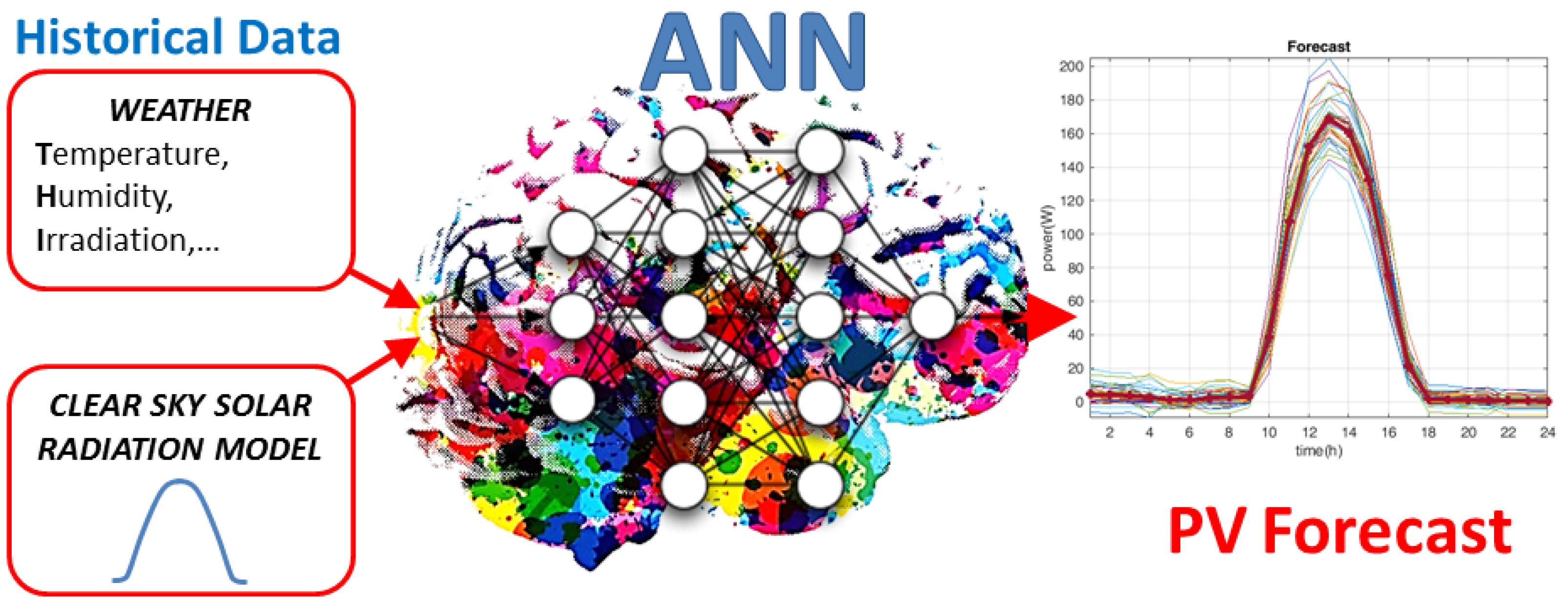
PHANN method, schematically represented in Figure 1, has been described in [30] and includes the physical Clear Sky Solar Radiation (CSRM) algorithm as an additional input with the previously mentioned ANN. This combination improves the forecasting of the PV output power generating a reliable hourly profile when the weather parameters, estimated 24 h in advance, are provided to a network trained with the historical data.
The capability of the nonlinear approximation of ANNs can easily result in bad generalization of trained ANN to new data, giving rise to chance effects. Since a network with a sufficient number of neurons in the hidden layer can exactly implement an arbitrary training set, it can learn both investigated dependencies and noise (worsening the predictive ability of the network). A probable description of overtraining is that the network learns the gross structure first and then the fine structure that is generated by noise [31].
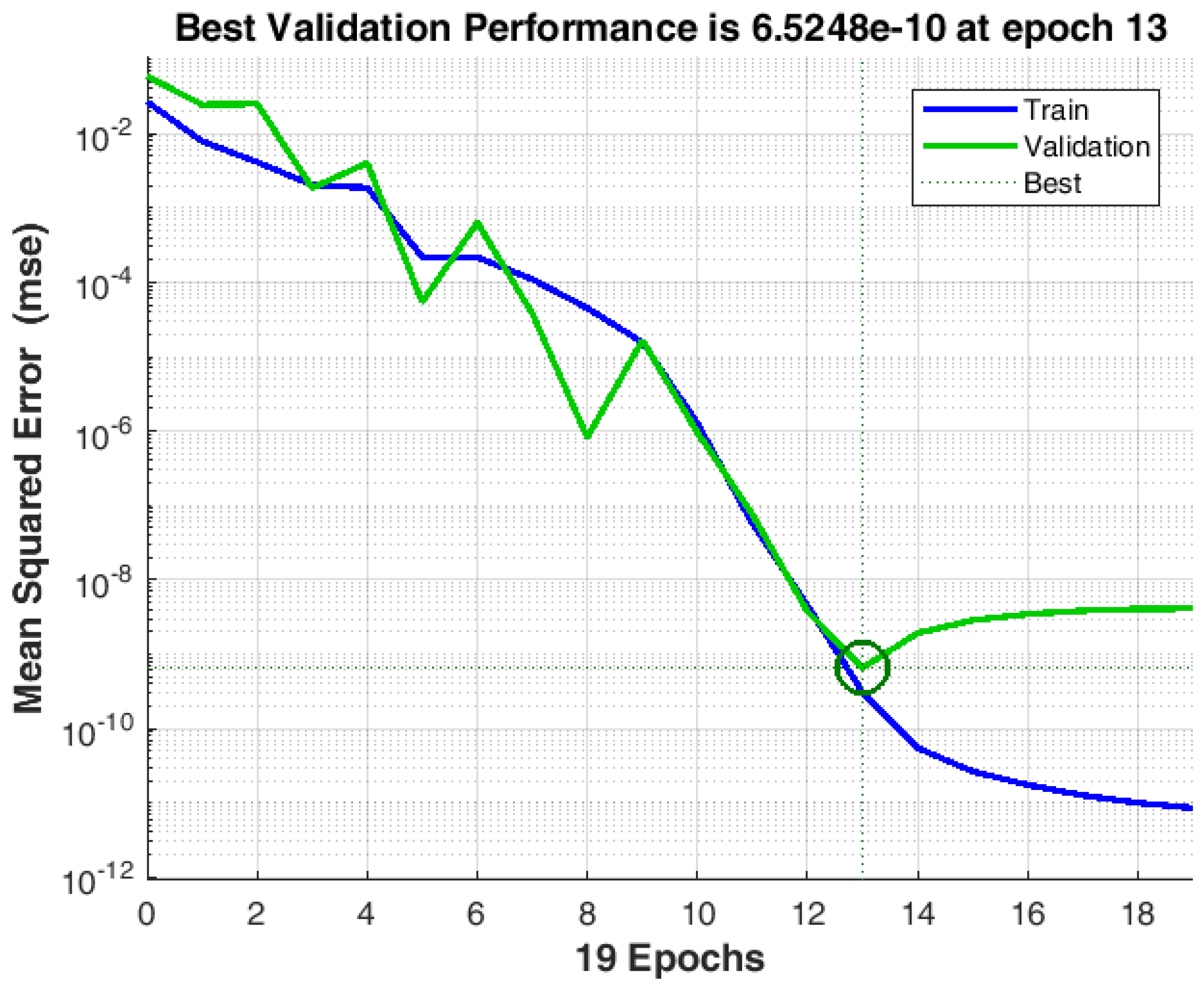
While the Mean Square Error (MSE) of a network for a learning set gradually decreases with time of training, predictive performance of the network has parabolic dependence, as it is shown in a generic example in Figure 2. It is optimal to stop net training before complete convergence has occurred (so called “early stopping”). A point when a network training should be stopped is determined by testing of the network on an additional test set (cross-validation method). In this work, by using the Neural Network ToolboxTM [32] in Matlab, which automatically includes these techniques, overfitting is avoided.
2.3. Physical Model Methodology
In this Section, the forecasting methodology based on the physical model estimated by means of Social Network Optimization (SNO) is described.
The physical model adopted is the five-parameter model and the parameters were estimated with SNO to fit a training set of data, in analogy with what was done with Neural Networks.
The procedure is summarized in Figure 3. SNO is an optimization algorithm that evolves a population of candidate solutions that represent the physical model parameters, according to some specific rules that takes their inspiration by Online Social Networks.
For each candidate solution, the weather forecasts contained in the training dataset are used to evaluate the power output by means of the physical model. This output is compared with the measured data contained in the same dataset, and with these data a cost value is returned to the algorithm.
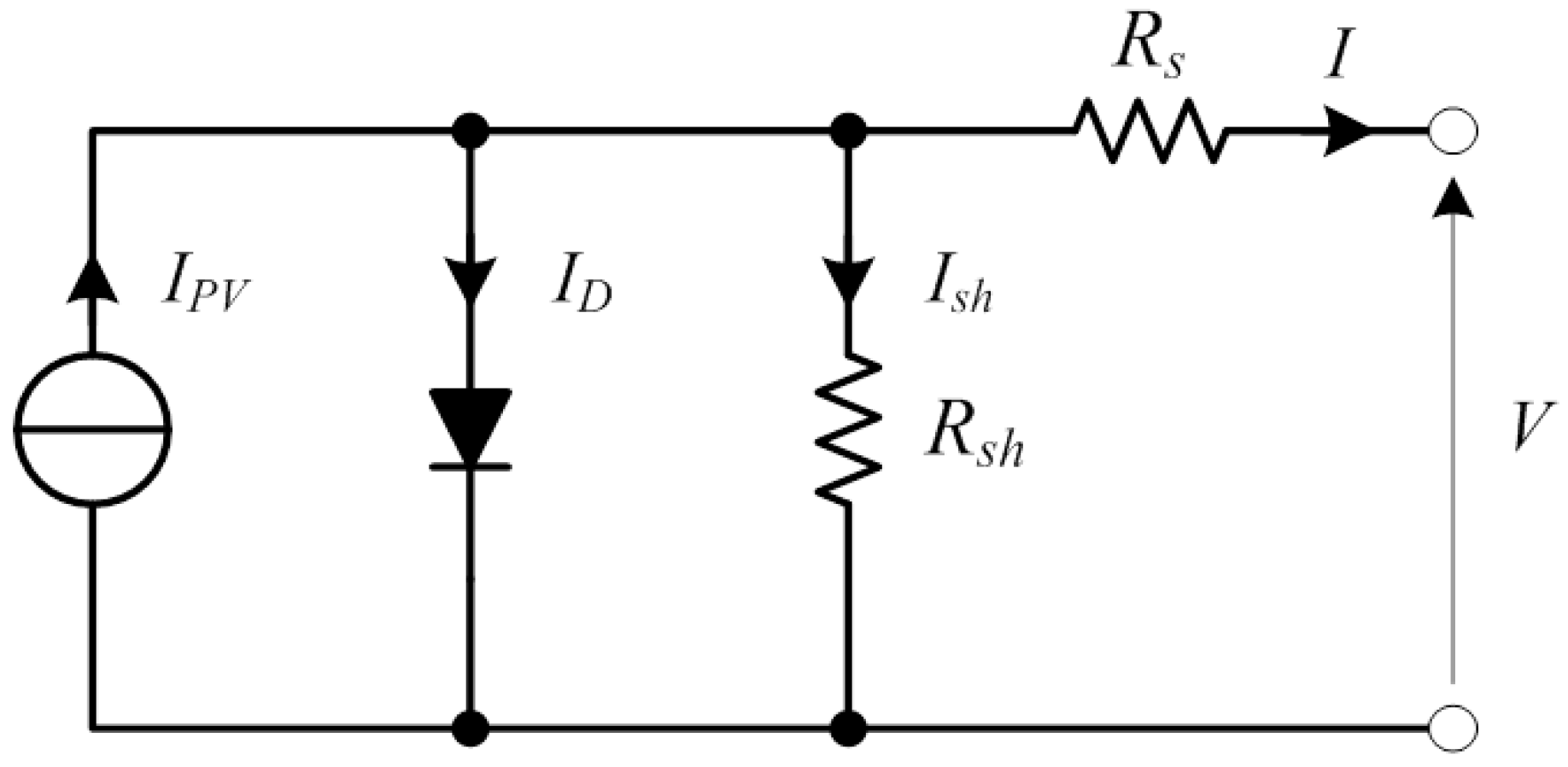
The physical model used is the five parameter model, which is able to obtain the I–V curve of a single cell from the irradiation and temperature data. It is possible to obtain the curve of the entire module combining the curves of each cell and bypass diode to comply with the series and parallel electrical connection constraints [21]. The equivalent circuit of this model is reported in Figure 4.
The five unknown parameters that characterize this model are the temperature voltage (), the leakage or reverse saturation current (), the diode quality factor (n), the series resistance () and the shunt resistance (). Referring to the equivalent electric circuit in Figure 4, the I–V curve of a PV cell can be expressed based on Kirchhoff’s current law, Ohm’s law and Shockley diode equation:
The light generated current, , as a function of irradiation, G, and cell temperature, , can be expressed as:
where the subscript ref stands for reference conditions and is the temperature coefficient for short-circuit current. In most cases, reference values are measured at standard test conditions (STC), that is with equal to 1000 W/m2 , cell temperature equal to 25 °C and Air Mass equal to 1.5. In this model, the variations of the five parameters with the cell temperature and the irradiation are neglected.
The adopted optimization algorithm is Social Network Optimization, a population-based evolutionary algorithm that takes its inspiration from the information sharing process of Online Social Networks [33]. The flow chart of SNO can be found in [34].
The population of SNO represents social network members, each one characterized by its status (i.e., the candidate solution of the problem), a personal character, a reputation (i.e., the cost associated to the candidate solution), and a personal interest that can drive the construction and the evolution of the relational network [35]. The individual’s character and interest are used as internal variables of the algorithm to evolve the population from one iteration to another.
The most important mechanisms taken from Online Social Networks are: the fact that the interaction is borrowed by the discernment capability of the social network itself and the natural division of people into groups. The discernment capability keeps track of the good solution found, and it aimd to find a good trade-off between the elitism and the possible stagnation produced when no new information is discovered. The interaction between people is the key aspect of the population evolution and it takes place in the groups. In each of them, all the individuals are influenced and they defined an ideal desired situation .
To get toward this desideratum, each individual changes his character and his situation according to the following equations:
where and are the actual and the future characters of the i-th individual, is the actual status of the i-th individual, and is his desideratum. and are two user-defined parameters.
The termination criterion adopted for SNO is the maximum number of cost function calls. This value is important because it is highly related with the computational time required. In this case, the early stopping for the validation criterion was not implemented because the reduced number of parameters and the high number of training samples guarantees avoiding overtraining.
2.4. Mixed Forecasting Method
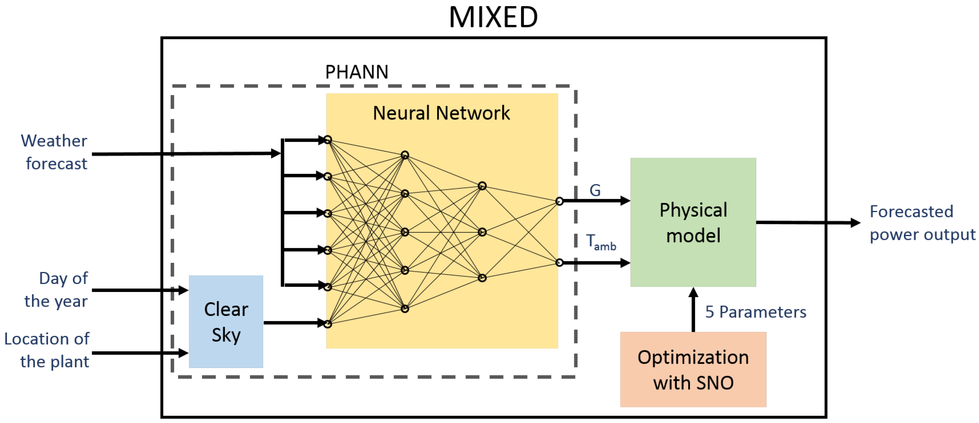
In this Section, the new proposed mixed forecasting method is described. In particular, this is a combination between PHANN and the five-parameter physical model trained by SNO.
This method has been implemented to improve the performance of the previous models. In fact, it is known that physical models are highly affected by the intrinsic inaccuracy of the weather forecasts which are, in this new method, enhanced by the learning capability of PHANN. Moreover, physical model receives only solar irradiation and ambient temperature in input while a larger amount of weather parameters are provided to PHANN.
These additional data can be used to improve the values of irradiation and temperature by means of a Neural Network. The proposed method is summarized in Figure 5. The model is composed as follows: the day of the year and the location of the power plant are provided as input of the clear sky. The output of it and the weather forecasts are given as input to an Neural Network that is trained to give as output weather conditions the closest to the measured ones. This part of the system is similar to PHANN. The improved weather forecast and the five parameter sestimated with SNO are given as input to the physical model that finally provides the forecasted power output.
3. Assessment Indicators
In this work, to perform the evaluation of the forecasting methods accuracy, some of the most common error indexes in the literature [36,37,38] have been applied.
The hourly error is defined as:
where is the mean actual power in the hour and is the prediction provided by one of the forecasting methods. Starting from this definition, other indexes have been introduced to have a more precise and reliable assessment of the methods:
- Normalized mean absolute error () is mean absolute error divided by the rated power of the PV module C expressed in watt:
- Envelope-weighted mean absolute error () [21] is defined as:
- Root mean square error () is used as the main error metric because it emphasizes the large errors:
- It can be also normalized when divided by the maximum output dc power measured in the whole period:
In all of these definitions, N is the number of hours in the evaluated period (i.e., 24 h in a daily error basis calculation).
These indexes are strongly correlated to each other [29] and a single index can be adopted in the analysis. This index can describe the global trend of the others (even if in a different scale). While estimating the five-parameter model with SNO, the choice of the error index can influence the quality of the results and that the definition is the most promising.
It is important to remember that forecast accuracies are not comparable site-by-site or hour-by-hour unless normalized by a benchmark. To face this problem, an additional metric has been introduced. This metric is the forecast skill and it is used to evaluate the improvement with respect to the baseline model (here the persistence model):
where is the for the forecasting model and for the persistence model.
4. Case Study
In this work, the models proposed have been compared using experimental data recorded at the laboratory SolarTechLab [25], Politecnico di Milano, the coordinates of which are latitude 45°30′10.588″ N and longitude 9°9′23.677″ E. The dc output power of a single PV module with the following characteristics was recorded:
- PV technology: Silicon mono crystalline
- Rated power: 285 Wp
- Azimuth: −6°30′ (assuming 0° as South direction and counting clockwise)
- Solar panel tilt angle: 30°
The PV module ratings are reported in Table 1. It is made of 60 cells connected in series and three bypass diodes, parallel connected to groups of 20 cells, dividing the PV module in three equal electrical sections.
The recording of the data lasted from 8 February to 14 December 2014, and from 4 January to 31 December 2017, but the employable data, without interruptions and discontinuities amount to 212 and 268 days, respectively. All the hourly recorded samples, including nights, are used as dataset for the comparison of the forecasting models.
The analyzed PV module is connected to the electric grid by means of a micro inverter, which guarantees the maximum power tracking variations of the production.
The employed weather forecasts are received from a weather service each day at 11:00 p.m. of the day before the forecasted one, hence 24 h ahead. The weather parameters provided and used to train the models, are: ambient temperature (, °C), Global Horizontal Solar radiation (GHI, W/m2), normal solar radiation on PV cell (G, W/m2), wind speed (m/s), wind direction (°), pressure (hPa), precipitation (mm), cloud cover (%) and cloud type (low/medium/high).
To train the PHANN method, the local time (hh:mm) of the day and the CSRM CSRM (W/m2) are also required. As regards the SNO based physical model, only the G solar irradiation and the ambient temperature are used for the forecasting.
5. Results and Discussion
In this Section, the results of the application of the proposed forecasting methods are provided. Several cases were analyzed in the present work. Their main characteristics are summarized in the Table 2.
For Cases (A) and (B), the historical data of the weather forecasts provided by a meteorological service were employed. In Case (C), to calculate the real methods accuracy, the forecasts were performed once by using actual measurements of the weather parameters and once using the weather forecasts.
5.1. Case (A)—Training Curves
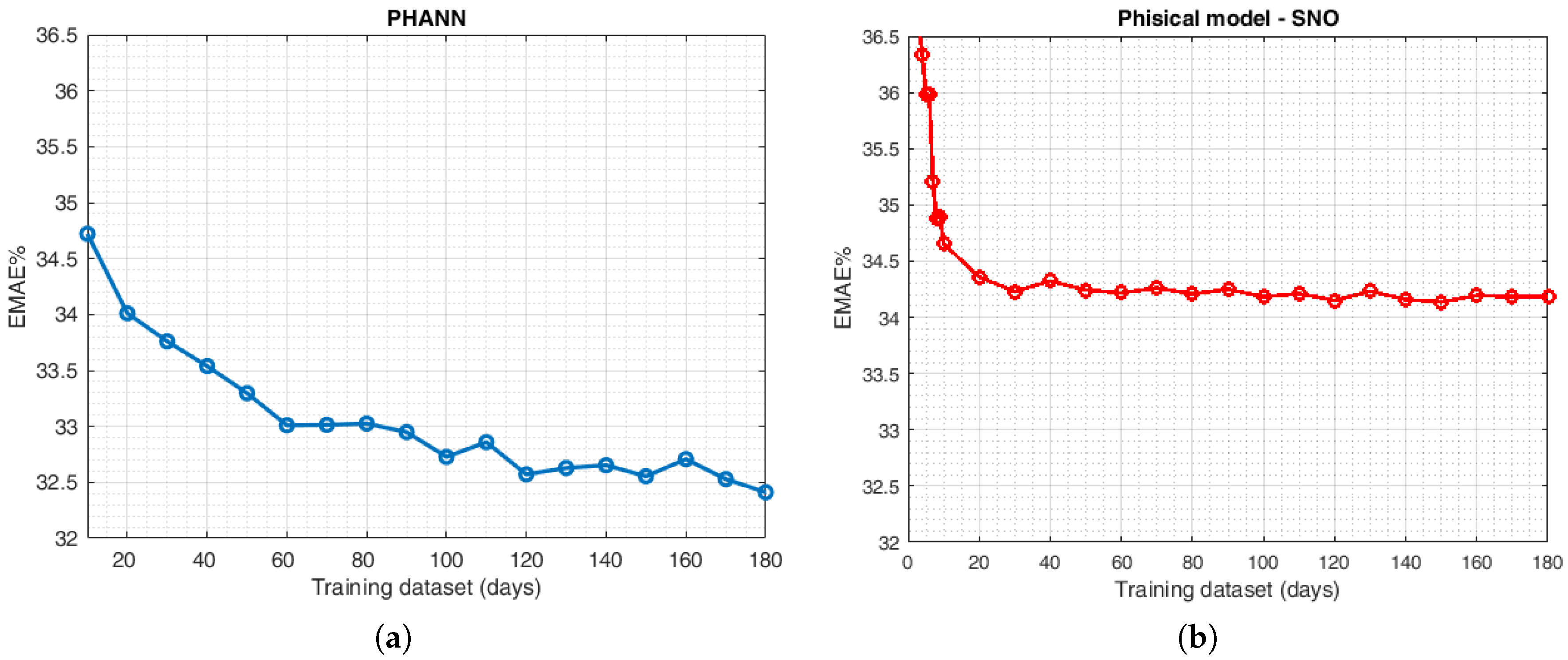
In this subsection, the training dataset size has been iteratively modified to identify the optimal amount of days that should be used for training the PHANN model and the SNO-based model.
The results are shown in Figure 6. Concerning PHANN method (Figure 6a), the increasing step size in the training is constant and equal to 10 days. As regards SNO (Figure 6b), the increasing steps were not kept constant. In fact, with few days available in the training, the variation in the error magnitude (EMAE%) is considerably high, therefore the curve is denser and the increasing step has been set to one day. For this reason, after 20 days in the training dataset, the increasing step is equal to 10 days.
For both models, for each dataset size, the training days were picked randomly, while the testing phase was conducted on all available days. The error value reported in Figure 6 is the average of the testing errors of 40 independent trials.
It is evident that the yearly EMAE% value is lower with PHANN than SNO (32.4% vs. 34.2%), however the results are comparable even if the shapes are different: PHANN training curve is asymptotically decreasing until it reaches the minimum with 180 days, and SNO reaches a constant value for more than 30 days, as reported in Table 3. From these data, it is possible to see that, even if the physical model is less accurate than PHANN, it can be adopted with less input, and consequently can be used when a large dataset is not available.
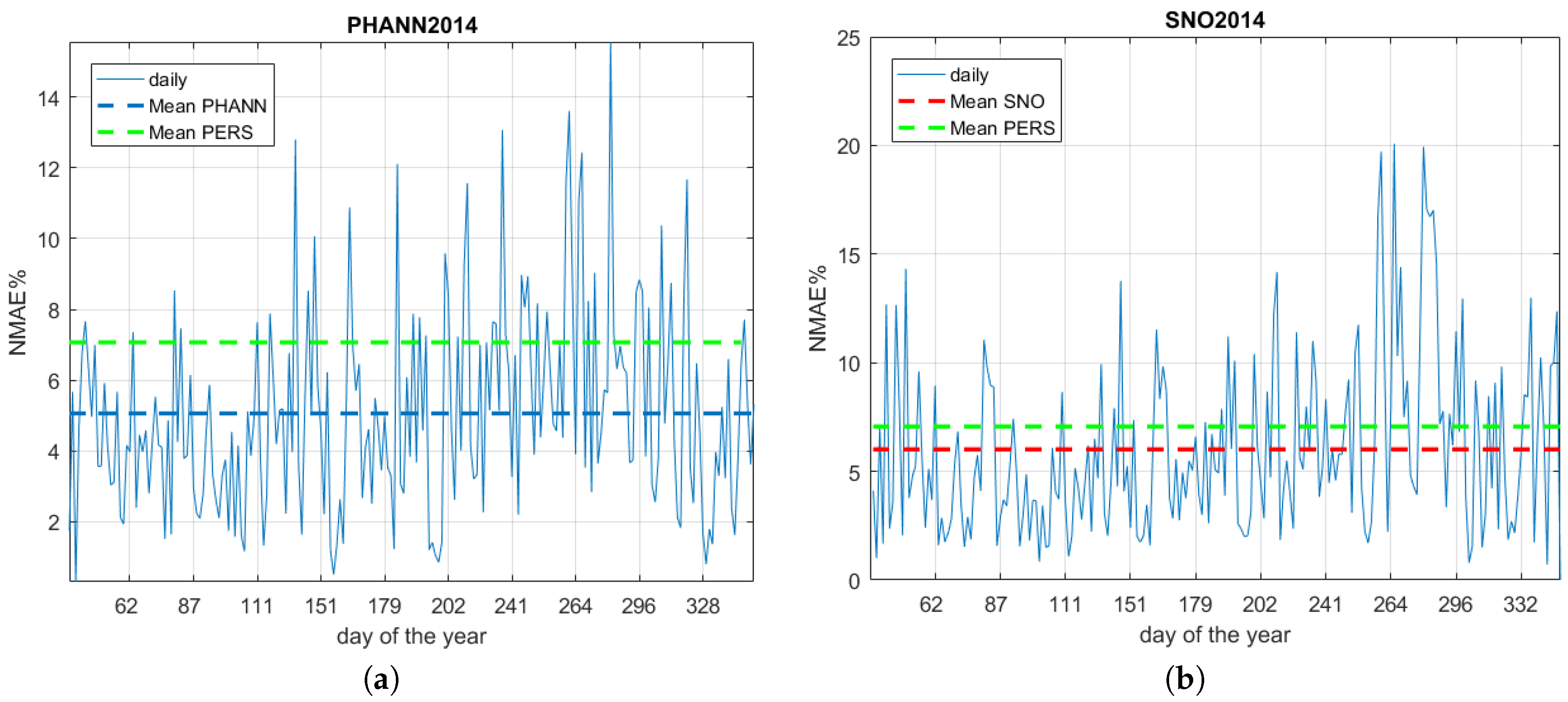
5.2. Case (B)—Daily Errors 2014
In this subsection, the daily results for 2014 are shown. The historical weather forecasts, delivered 24 h in advance, have been employed for this analysis. This is a peculiar aspect which should be considered when evaluating a forecasting method; in fact, the method accuracy is strongly affected by the weather forecasts inaccuracy.
This is important when considering the forecasting method; in fact, it is well-known that “white box” methods, i.e., physical models, are more influenced by the weather data inaccuracies that are used. On the contrary, “black-box” based methods suffer less, as they are capable of learning peculiar trends and intrinsic inaccuracies on the parameters that are employed for the training.
The results for 2014 of the daily errors are shown in Figure 7a for PHANN and Figure 7b for SNO, with the mean yearly values reported with dashed lines. The Persistence model scored a yearly NMAE% equal to 7.06%, which is higher than the other considered methods: 5.05% for PHANN and 6.01% for SNO based model. The same trends are found in all error indicators.
In Figure 7, it is possible to see that both PHANN and SNO perform better than the persistence model and that PHANN is the best. Analyzing the daily error curves, it is possible to see that both models have a peak of the error in the second half of the year. This trend is more evident for PHANN, while the error in SNO-based model is concentrated in few days.
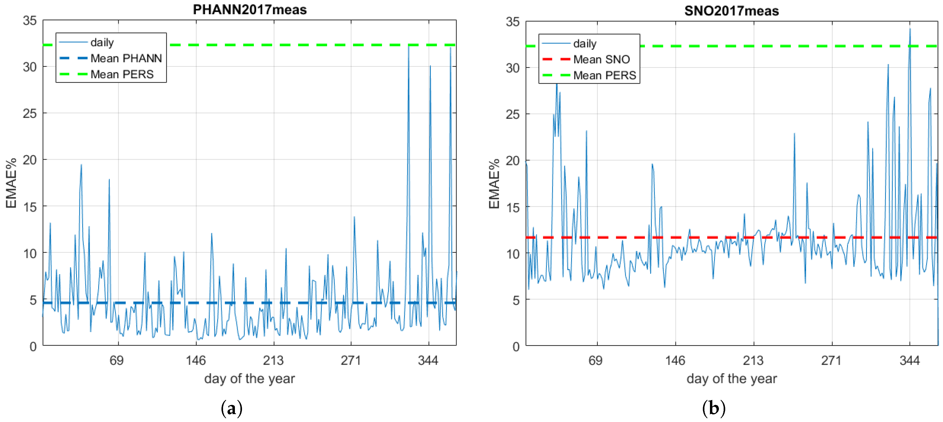
5.3. Case (C)—Daily Errors 2017
This analysis aimed at testing the real forecasting methods accuracies; therefore, weather measurements were employed in the training. After this preliminary assessment, both methods were also evaluated in regular forecasting conditions, i.e., with weather forecasts delivered 24 h in advance.
The results of the first assessment are shown in Figure 8a for PHANN and Figure 8b for SNO based model. The EMAE% yearly mean values are depicted with dashed lines in blue and red, respectively, while the persistence is in green. It is evident that both analyzed models perform better than persistence (32.3%), however SNO based model is less accurate (11.6%) than PHANN (4.6%).
The second analysis led to adopting the weather forecasts in the training and the results are shown in Figure 9. As already shown with 2014 data, PHANN is still better if compared to both SNO based model and persistence.
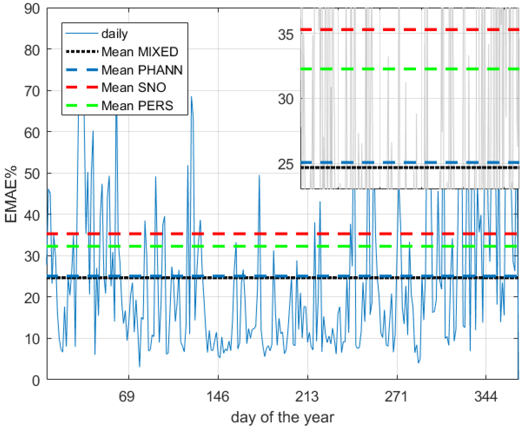
Comparing the worsening of the performance from the measured weather data to the forecasted ones, it is possible to see that the physical model is most affected. To improve the results, the mixed model has been introduced. As explained before, this model combines the weather forecast parameters (G, T) obtained by a PHANN with the five-parameter model estimated by SNO.
The results of this model are summarized in Figure 10, where the daily errors (EMAE%) of the mixed method are shown and the mean EMAE% calculated over the whole 2017 for all methods analyzed are depicted. In particular, the subplot in the upper right corner of Figure 10 shows that the mixed method outperforms all the others (EMAE% equal to 24.67). All the error indicators are reported in Table 4.
More in detail, the forecast skill of all methods are listed in Table 4. It can be seen that the mixed forecasting method here presented scored the highest forecasting skill, equal to 47%, with PHANN second (37%), followed by SNO (5%).
From these data, it is possible to notice that the mixed method behaves generally better than the others. In the following, some peculiar days are analyzed.
5.4. Focus on Peculiar Days
The results above refer to an entire year of analysis. Here, the attention is focused on some peculiar days to better understand the behavior of the three forecasting methods.
The analyzed days have been chosen to have different typologies of days. With reference to the weather conditions, three behaviors have been extracted: a cloudy day, a sunny day and a day with great variations in the weather conditions. With reference to the performance of the proposed mixed method, the best case and the worst case are shown. In particular, both the best and the worst cases are sunny days, so they are representative both of the performance and of the weather forecast.
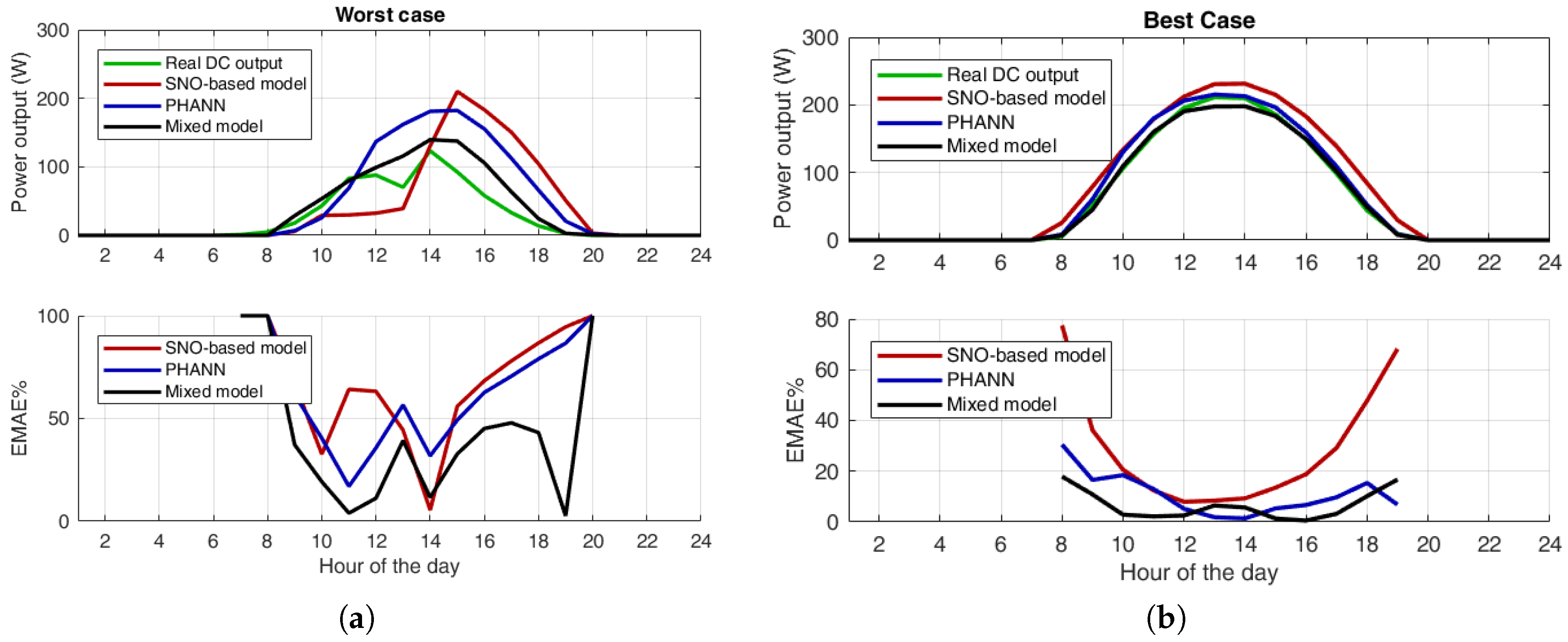
The best and the worst days in terms of the performances of the mixed model are shown in Figure 11. Analyzing these results, it is possible to see that, in both cases, the mixed model is the best performing, even if Figure 11a shows the day in which the average EMAE of the mixed model is the worst one. Analyzing the specific behviour, it is possible to see that the SNO-based model is able to estimate the sudden variation of the DC power output, but it is not able to correctly evaluate the amount of this variation; on the other hand, the PHANN model is completely missing the variation. The mixed model has a behavior that is in between and, thus, can reproduce better the real trend.
Analyzing the best day in terms of performance, shown in Figure 11b, it is possible to see that all three models are very accurate, but the mixed model is able to drastically reduce the EMAE% at the beginning and at the end of the day.
It is important to consider two points about the error trend. Firstly, the error index adopted is the EMAE, which is defined only when the forecasted power or the measured one is non-zero. This means that the curves are not defined during the night, when both the powers are null. Secondly, at the beginning and at the end of the day, EMAE reaches 100% because either the forecast or the measure equals zero in that hour.
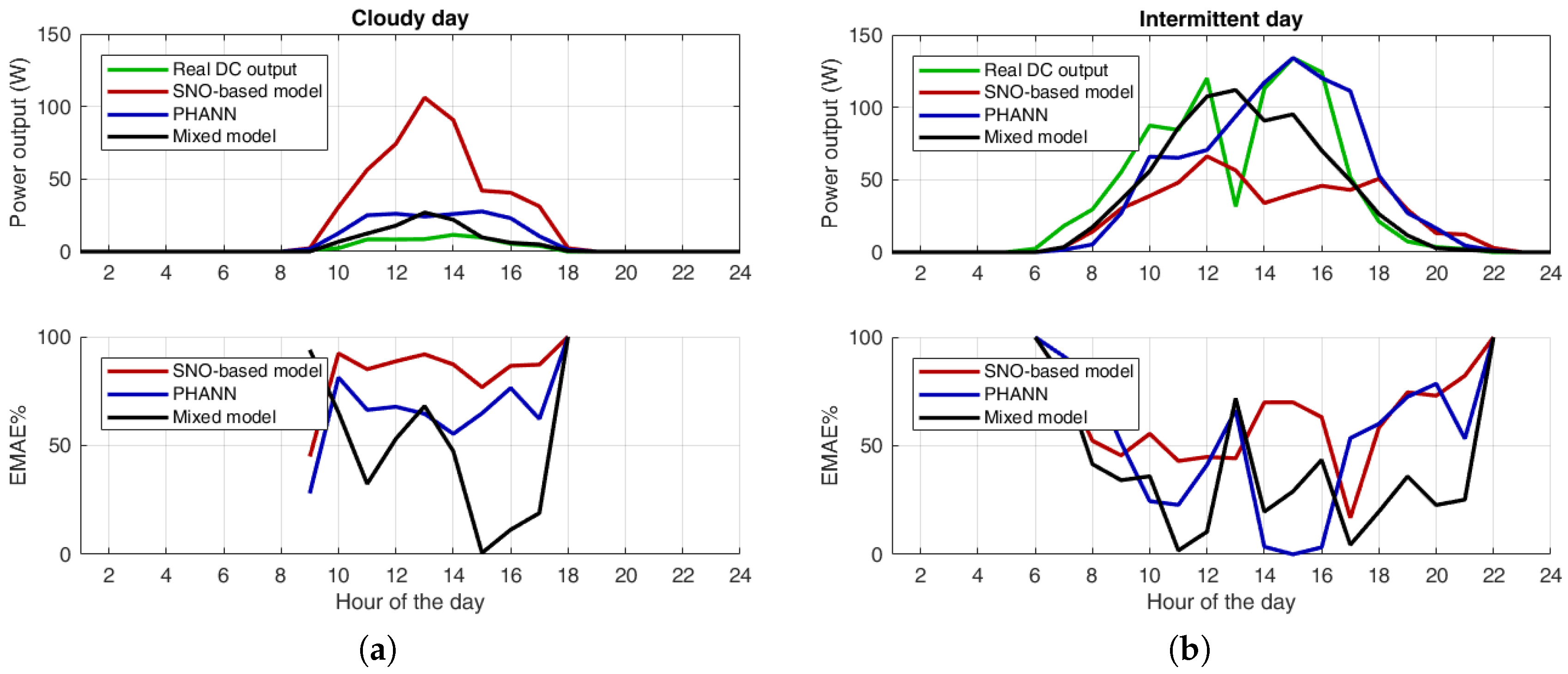
The behavior of the power output for a cloudy day and a variable day are shown in Figure 12. Analyzing Figure 12a, it is possible to see that the SNO-based model is absolutely not able to forecast the behavior of the power output. The PHANN method and the mixed one are equivalent in the central hours of the day, but the mixed is much more precise in the middle morning and in the middle afternoon. The intermittent day shown in Figure 12b shows that none of the models are able to follow the valley at 1:00 p.m. This problem is due to the unpredictable nature of that event that has not been identified by the forecasting system.
6. Conclusions
In this paper, a new method for the day-ahead PV output power forecast has been presented. This “mixed method” includes the main features of two other methods: a hybrid physical-stochastic model based on Artificial Neural Network (PHANN), and a physical model where the parameters have been estimated with Social Network Optimization (SNO). The aim of this “mixed method” is to improve the weather forecasts with PHANN and to optimize the five-parameter model with SNO.
The persistence method was adopted as a benchmark and the results of all the considered methods were compared baed on the experimental data from a real PV module. In this analysis, both the weather measurements and forecasts were employed.
Firstly, historical data belonging to 2014 were employed for a deep analysis of the different algorithms, both in terms of training curves, as a function of the number of days in the dataset, and in terms of daily errors. From the error curves of the increasing training set size, it is shown that, even if PHANN generally performs better than the other methods, SNO requires a smaller training set to reach its optimal performance. As regards the forecasting errors, it is shown that the persistence forecast is less accurate than the others while PHANN shows the best results, in both the yearly errors and the daily errors.
In addition, PHANN and SNO-based methods were separately compared by excluding possible inaccuracies of the weather forecasts which can strongly affect one of the methods. In this analysis, actual weather measurements were employed as input for the forecasting model. In this analysis, PHANN generally performed better than the other methods.
Instead, the third analysis aimed at comparing the forecasting methods under regular operating conditions. Here, the hybrid model PHANN shows its ability to outperform the physical model in different testing conditions on different years. In this assessment, the errors of SNO based model is comparable with persistence (slightly better in 2014, while worse in 2017).
The final mixed forecasting model, tested with the weather forecast of 2017, shows the best performance, especially in terms of forecasting skills. This is a promising method because it enhanced the PHANN forecasting capability combining it with the performing optimization characteristics of SNO.
Further activities for improving this work are related with the collection of data in other sites with different weather conditions. This activity is aimed to better assess the forecasting capabilities of the proposed method.
Author Contributions
In this research activity, all of the authors were involved in the data analysis and preprocessing phase, the simulation, the results analysis and discussion, and the manuscript preparation. Conceptualization, E.O. and A.N.; Methodology, E.O. and A.N.; Validation, S.L., and R.E.Z; Formal Analysis, S.L.; Investigation, R.E.Z.; Data Curation, E.O.; Writing—Original Draft Preparation, A.N.; Writing—Review & Editing, E.O. and A.N.; Supervision, R.E.Z.; Project Administration, S.L.
Conflicts of Interest
The authors declare no conflict of interest.
References
- Price, L.; Michaelis, L.; Worrell, E.; Khrushch, M. Sectoral trends and driving forces of global energy use and greenhouse gas emissions. Mitig. Adapt. Strategies Glob. Chang. 1998, 3, 263–319. [Google Scholar] [CrossRef]
- Wan, C.; Zhao, J.; Song, Y.; Xu, Z.; Lin, J.; Hu, Z. Photovoltaic and solar power forecasting for smart gridenergy management. CSEE J. Power Energy Syst. 2015, 1, 38–46. [Google Scholar] [CrossRef]
- Ferruzzi, G.; Cervone, G.; Delle Monache, L.; Graditi, G.; Jacobone, F. Optimal bidding in a Day-Ahead energymarket for Micro Grid under uncertainty in renewable energy production. Energy 2016, 106, 194–202. [Google Scholar] [CrossRef]
- Hanna, R.; Kleissl, J.; Nottrott, A.; Ferry, M. Energy dispatch schedule optimization for demand charge reduction using a photovoltaic-battery storage system with solar forecasting. Sol. Energy 2014, 103, 269–287. [Google Scholar] [CrossRef]
- Yang, D.; Kleissl, J.; Gueymard, C.A.; Pedro, H.T.; Coimbra, C.F. History and trends in solar irradiance and PV power forecasting: A preliminary assessment and review using text mining. Sol. Energy 2018. [Google Scholar] [CrossRef]
- Bacher, P.; Madsen, H.; Nielsen, H.A. Online short-term solar power forecasting. Sol. Energy 2009, 83, 1772–1783. [Google Scholar] [CrossRef] [Green Version]
- Voyant, C.; Notton, G.; Kalogirou, S.; Nivet, M.L.; Paoli, C.; Motte, F.; Fouilloy, A. Machine learning methods for solar radiation forecasting: A review. Renew. Energy 2017, 105, 569–582. [Google Scholar] [CrossRef]
- Antonanzas, J.; Osorio, N.; Escobar, R.; Urraca, R.; Martinez-de Pison, F.; Antonanzas-Torres, F. Review of photovoltaic power forecasting. Sol. Energy 2016, 136, 78–111. [Google Scholar] [CrossRef]
- Raza, M.Q.; Nadarajah, M.; Ekanayake, C. On recent advances in PV output power forecast. Sol. Energy 2016, 136, 125–144. [Google Scholar] [CrossRef]
- Inman, R.H.; Pedro, H.T.; Coimbra, C.F. Solar forecasting methods for renewable energy integration. Prog. Energy Combust. Sci. 2013, 39, 535–576. [Google Scholar] [CrossRef]
- Graditi, G.; Ferlito, S.; Adinolfi, G. Comparison of Photovoltaic plant power production predictionmethods using a large measured dataset. Renew. Energy 2016, 90, 513–519. [Google Scholar] [CrossRef]
- Simon, D. Evolutionary Optimization Algorithms; John Wiley & Sons: Hoboken, NJ, USA, 2013. [Google Scholar]
- Cao, L.; Xu, L.; Goodman, E.D. A guiding evolutionary algorithm with greedy strategy for global optimization problems. Comput. Intell. Neurosci. 2016, 2016. [Google Scholar] [CrossRef] [PubMed]
- Davis, L. Handbook of Genetic Algorithms; Van Nostrand Reinhold: New York, NY, USA, 1991. [Google Scholar]
- Kennedy, J. Particle swarm optimization. In Encyclopedia of Machine Learning; Springer Science & Business Media: Berlin, Germany, 2011; pp. 760–766. [Google Scholar]
- Zou, F.; Chen, D.; Wang, J. An improved teaching-learning-based optimization with the social character of PSO for global optimization. Comput. Intell. Neurosci. 2016, 2016, 18. [Google Scholar] [CrossRef] [PubMed]
- Simon, D. Biogeography-based optimization. IEEE Trans. Evol. Comput. 2008, 12, 702–713. [Google Scholar] [CrossRef]
- Albi, R.; Grimaccia, F.; Mussetta, M.; Niccolai, A.; Zich, R. A new algorithm for antenna optimization in aerospace applications: The sounding rocket test case. In Proceedings of the 2013 International Conference on Electromagnetics in Advanced Applications (ICEAA), Torino, Italy, 9–13 September 2013; pp. 1537–1540. [Google Scholar]
- Oliva, D.; Cuevas, E.; Pajares, G. Parameter identification of solar cells using artificial bee colony optimization. Energy 2014, 72, 93–102. [Google Scholar] [CrossRef]
- Askarzadeh, A.; Rezazadeh, A. Artificial bee swarm optimization algorithm for parameters identification of solar cell models. Appl. Energy 2013, 102, 943–949. [Google Scholar] [CrossRef]
- Siddiqui, M.; Abido, M. Parameter estimation for five-and seven-parameter photovoltaic electrical models using evolutionary algorithms. Appl. Soft Comput. 2013, 13, 4608–4621. [Google Scholar] [CrossRef]
- Soon, J.J.; Low, K.S. Photovoltaic model identification using particle swarm optimization with inverse barrier constraint. IEEE Trans. Power Electron. 2012, 27, 3975–3983. [Google Scholar] [CrossRef]
- Ogliari, E.; Dolara, A.; Manzolini, G.; Leva, S. Physical and hybrid methods comparison for the day ahead PV output power forecast. Renew. Energy 2017, 113, 11–21. [Google Scholar] [CrossRef] [Green Version]
- Dolara, A.; Grimaccia, F.; Leva, S.; Mussetta, M.; Ogliari, E. Comparison of Training Approaches for Photovoltaic Forecasts by Means of Machine Learning. Appl. Sci. 2018, 8, 228. [Google Scholar] [CrossRef]
- SolarTech Lab. Politecnico di Milano, Milano, Italy, 2013. Available online: http://www.energia.polimi.it/en/energy-department/laboratories/research/solar-tech/ (accessed on 4 June 2018).
- Grimaccia, F.; Leva, S.; Mussetta, M.; Ogliari, E. ANN sizing procedure for the day-ahead output power forecast of a PV plant. Appl. Sci. 2017, 7, 622. [Google Scholar] [CrossRef]
- Krose, B.; van der Smagt, P. Back-propagation. In An introduction to Neural Networks, 8th ed.; University of Amsterdam: Amsterdam, The Netherlands, 1996; pp. 35–36. [Google Scholar]
- Ferlito, S.; Adinolfi, G.; Graditi, G. Comparative analysis of data-driven methods online and offline trained to the forecasting of grid-connected photovoltaic plant production. Appl. Energy 2017, 205, 116–129. [Google Scholar] [CrossRef]
- Gandelli, A.; Grimaccia, F.; Leva, S.; Mussetta, M.; Ogliari, E. Hybrid model analysis and validation for PV energy production forecasting. In Proceedings of the 2014 International Joint Conference on Neural Networks (IJCNN), Beijing, China, 6–11 July 2014; pp. 1957–1962. [Google Scholar]
- Dolara, A.; Grimaccia, F.; Leva, S.; Mussetta, M.; Ogliari, E. A physical hybrid artificial neural network for short term forecasting of PV plant power output. Energies 2015, 8, 1138–1153. [Google Scholar] [CrossRef] [Green Version]
- Tetko, I.V.; Livingstone, D.J.; Luik, A.I. Neural network studies. 1. Comparison of overfitting and overtraining. J. Chem. Inf. Comput. Sci. 1995, 35, 826–833. [Google Scholar] [CrossRef]
- Beale, M.H.; Hagan, M.T.; Demuth, H.B. Neural Network ToolboxTM User’s Guide; The Mathworks Inc.: Natick, MA, USA, 1992. [Google Scholar]
- Niccolai, A.; Grimaccia, F.; Mussetta, M.; Pirinoli, P.; Bui, V.H.; Zich, R.E. Social network optimization for microwave circuits design. Prog. Electromagn. Res. 2015, 58, 51–60. [Google Scholar] [CrossRef]
- Grimaccia, F.; Gruosso, G.; Mussetta, M.; Niccolai, A.; Zich, R.E. Design of tubular permanent magnet generators for vehicle energy harvesting by means of social network optimization. IEEE Trans. Ind. Electron. 2018, 65, 1884–1892. [Google Scholar] [CrossRef]
- Ruello, M.; Niccolai, A.; Grimaccia, F.; Mussetta, M.; Zich, R.E. Black-hole PSO and SNO for electromagnetic optimization. In Proceedings of the 2014 IEEE Congress on Evolutionary Computation (CEC), Beijing, China, 6–11 July 2014; pp. 1912–1916. [Google Scholar]
- Monteiro, C.; Fernandez-Jimenez, L.A.; Ramirez-Rosado, I.J.; Muñoz-Jimenez, A.; Lara-Santillan, P.M. Short-term forecasting models for photovoltaic plants: Analytical versus soft-computing techniques. Math. Probl. Eng. 2013, 2013. [Google Scholar] [CrossRef]
- Ulbricht, R.; Fischer, U.; Lehner, W.; Donker, H. First steps towards a systematical optimized strategy for solar energy supply forecasting. In Proceedings of the 2013 ECML/PKDD International Workshop on Data Analytics for Renewable Energy Integration (DARE), Prague, Czech Republic, 23–27 September 2013; pp. 14–25. [Google Scholar]
- Kleissl, J. Solar Energy Forecasting and Resource Assessment; Academic Press: Cambridge, MA, USA, 2013. [Google Scholar]
Figure 1.
PHANN basic scheme.

Figure 2.
Best PHANN performance avoiding overfitting.

Figure 3.
Diagram of the optimization process: interaction between the optimizer and the physical model.
Figure 3.
Diagram of the optimization process: interaction between the optimizer and the physical model.

Figure 4.
Diagram of the simulated off grid PV system.

Figure 5.
Block diagram of the mixed model.

Figure 6.
Training curves for 2014: (a) PHANN; and (b) physical model (SNO).

Figure 7.
Daily NMAE% for 2014: (a) PHANN; and (b) SNO based model.

Figure 8.
Daily EMAE% for 2017 using measured weather data: (a) PHANN; and (b) SNO based model.

Figure 9.
Daily EMAE% for 2017 using weather forecasts: (a) PHANN; and (b) SNO based model.

Figure 10.
Daily EMAE% for 2017 for the mixed method and mean values of all forecasting methods.

Figure 11.
Comparison between the SNO-based model, the PHANN and the mixed model on the best and the worst days in terms of power output and % error trend: (a) Worst performance day; and (b) Best performance day.
Figure 11.
Comparison between the SNO-based model, the PHANN and the mixed model on the best and the worst days in terms of power output and % error trend: (a) Worst performance day; and (b) Best performance day.

Figure 12.
Comparison between the SNO-based model, the PHANN and the mixed model on a cloudy day and on an intermittent day in terms of power output and % error trend: (a) cloudy day; and (b) intermittent day.
Figure 12.
Comparison between the SNO-based model, the PHANN and the mixed model on a cloudy day and on an intermittent day in terms of power output and % error trend: (a) cloudy day; and (b) intermittent day.


Table 1.
PV module electrical data.
| Electrcal Data | STC 1 | NOCT 2 | |
|---|---|---|---|
| Rated Power | (W) | 285 | 208 |
| Rated Voltage | (V) | 31.3 | 28.4 |
| Rated Current | (A) | 9.10 | 7.33 |
| Open-Circuit Voltage | (V) | 39.2 | 36.1 |
| Short-Circuit Current | (A) | 9.73 | 7.87 |
1 Electrical values measured under Standard Test Conditions: 1000 W/m2, cell temperature 25 °C, AM 1.5; 2 Electrical values measured under Nominal Operating Conditions of cells: 800 W/m2, ambient temperature 20 °C, AM 1.5, wind speed 1 m/s, NOCT: 48 °C (nominal operating cell temperature).
Table 2.
Summary of the test cases.
| Analysis | Year | Methods | Weather Data | |
|---|---|---|---|---|
| (A) | Training curves | 2014 | SNO, PHANN | Forecasts |
| (B) | Daily Errors | 2014 | SNO, PHANN | Forecasts |
| (C) | Daily Errors | 2017 | SNO, PHANN, Mixed | Measurements, Forecasts |
Table 3.
Results of Case (A).
| Min EMAE % | Corresponding Days of Training | Independent Trials | |
|---|---|---|---|
| PHANN | 32.4 | 180 | 40 |
| SNO | 34.4 | >20 | 40 |
Table 4.
Results of case C.
| NMAE % | nRMSE % | EMAE % | s % | |
|---|---|---|---|---|
| PERS | 5.63 | 34.38 | 32.59 | 0 |
| PHANN | 3.79 | 21.52 | 25.07 | 37 |
| SNO | 6.94 | 32.78 | 35.33 | 5 |
| MIXED | 4.48 | 18.16 | 24.67 | 47 |
© 2018 by the authors. Licensee MDPI, Basel, Switzerland. This article is an open access article distributed under the terms and conditions of the Creative Commons Attribution (CC BY) license (http://creativecommons.org/licenses/by/4.0/).
Share and Cite
MDPI and ACS Style
Ogliari, E.; Niccolai, A.; Leva, S.; Zich, R.E. Computational Intelligence Techniques Applied to the Day Ahead PV Output Power Forecast: PHANN, SNO and Mixed. Energies 2018, 11, 1487. https://doi.org/10.3390/en11061487
AMA Style
Ogliari E, Niccolai A, Leva S, Zich RE. Computational Intelligence Techniques Applied to the Day Ahead PV Output Power Forecast: PHANN, SNO and Mixed. Energies. 2018; 11(6):1487. https://doi.org/10.3390/en11061487
Chicago/Turabian StyleOgliari, Emanuele, Alessandro Niccolai, Sonia Leva, and Riccardo E. Zich. 2018. "Computational Intelligence Techniques Applied to the Day Ahead PV Output Power Forecast: PHANN, SNO and Mixed" Energies 11, no. 6: 1487. https://doi.org/10.3390/en11061487
Note that from the first issue of 2016, this journal uses article numbers instead of page numbers. See further details here.