Abstract
We have developed an unsteady and non-linear wind synopsis simulator called RIAM-COMPACT (Research Institute for Applied Mechanics, Kyushu University, COMputational Prediction of Airflow over Complex Terrain) to simulate the airflow on a micro scale, i.e., a few tens of km or less. In RIAM-COMPACT, the large-eddy simulation (LES) has been adopted for turbulence modeling. LES is a technique in which the structures of relatively large eddies are directly simulated and smaller eddies are modeled using a sub-grid scale model. In the present study, we conducted numerical wind diagnoses for the Taikoyama Wind Farm nacelle separation accident in Japan. The simulation results suggest that all six wind turbines at Taikoyama Wind Farm are subject to significant influence from separated flow (terrain-induced turbulence) which is generated due to the topographic irregularities in the vicinity of the wind turbines. A proposal was also made on reconstruction of the wind farm.
1. Introduction
At Taikoyama Wind Farm (located on Mt. Taikoyama, Kyoto Prefecture, Japan) at around 19:30 on 12 March 2013, a major accident occurred in which a portion of Wind Turbine (WT) No. 3 constituting the generator and blades (height: approximately 50.0 m; weight: approximately 45.0 t) fell to the ground. The base of the nacelle, which connects the tower and the blades, was fractured. Since the wind speed at the time of the accident was about 15.0 m/s and was within the design limit, investigations were conducted based on a standpoint that metal fatigue was the main cause of the accident. A report [1] on the investigation results has already been made available to the public, and the results are also reported in the literature [2].
There are six 750 kW wind turbines manufactured by Lagerwey in the Netherlands at Taikoyama Wind Farm. The maximum output of the wind farm is 4500 kW. The annual energy output of the wind farm projected in the planning stage was 8549 MWh. The wind farm has been operated by a government affiliated public utility organization in Kyoto Prefecture since November 2001. The total operating cost of the wind farm is approximately 1.5 billion yen. The annual mean wind speed evaluated at the time of the detailed investigation of the wind conditions was 5.4 m/s at the height of 20.0 m above the ground surface. (The annual mean wind speed corrected to the 50.0 m height with a power law exponent of 1/7 was 6.2 m/s.) Figure 1, Figure 2 and Figure 3 show the location of the Taikoyama Wind Farm, a still image of the wind farm from the time of the accident, and a schematic diagram of the wind turbines, respectively.

Figure 1.
Location of Taikoyama Wind Farm in Kyoto Prefecture, Japan.
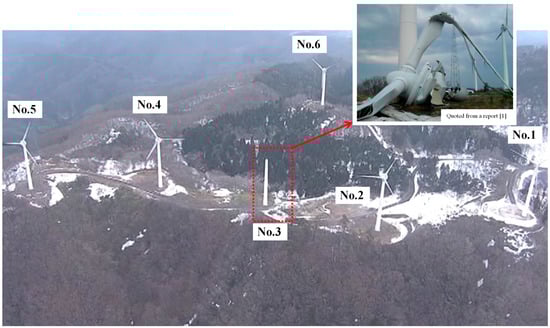
Figure 2.
Still image of wind turbine accident, taken from a video by RKB Mainichi Broadcasting Corporation.
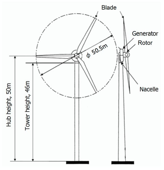
Figure 3.
Schematic diagram of the wind turbine.
Liu and Ishihara [2] did not report details of the airflow characteristics at each wind turbine site. Accordingly, the present study focused on the effect of the terrain-induced turbulence which is generated in the vicinity of the wind turbines, and conducted unsteady, numerical wind diagnoses for Taikoyama Wind Farm using LES technique [3,4,5,6,7,8,9]. Based on the numerical simulation results, relative comparisons were made of the airflow characteristics among the wind turbine locations. In particular, the present study focused on: (1) the three-dimensional structure of the airflow; and (2) the standard deviations of the three components (i.e., streamwise, spanwise, and vertical components) of the wind velocity that were evaluated from time-series data. In the present paper, “terrain-induced turbulence” is defined as “temporal and spatial fluctuations of airflow which are generated by topographic irregularities.”
2. Overview of Numerical Simulation Method
The present study used the RIAM-COMPACT natural terrain version software package [3,4,5,6,7,8,9], which is based on a collocated grid in a general curvilinear coordinate system, to numerically predict local wind flow over complex terrain with high accuracy while avoiding numerical instability. In this collocated grid, the velocity components and pressure are defined at the grid cell centers, and variables that result from multiplying the contravariant velocity components by the Jacobian are defined at the cell faces. For the numerical technique, the finite-difference method (FDM) was adopted, and a large-eddy simulation (LES) model was used for the turbulence model. In the LES model, a spatial filter is applied to the flow field to separate eddies of various scales into grid-scale (GS) components, which are larger than the computational grid cells, and sub-grid scale (SGS) components, which are smaller than the computational grid cells. Large-scale eddies, i.e., the GS components of turbulence eddies, were directly numerically simulated without the use of a physically simplified model. In contrast, dissipation of energy, which is the main effect of small-scale eddies, i.e., the SGS components, was modeled according to a physics-based analysis of the SGS stress.
For the governing equations of the flow, a filtered continuity equation for incompressible fluid (Equation (1)) and a filtered Navier–Stokes equation (Equation (2)) were used. Because high wind conditions, with mean wind speeds of 8.0 m/s or higher, are considered in the present study, the effect of vertical thermal stratification (atmospheric stability), which is generally present in the atmosphere, was neglected. As in Uchida et al. [3,4,5,6,7,8,9], the effects of the surface roughness were considered by reconstructing surface irregularities in high resolution. For the computational algorithm, a method similar to a fractional step (FS) method [10] was used, and a time marching method based on the Euler explicit method was adopted. The Poisson’s equation for pressure was solved by the successive over-relaxation (SOR) method. For discretization of all the spatial terms except for the convective term in Equation (2), a second-order central difference scheme was applied. For the convective term, a third-order upwind difference scheme was applied. An interpolation technique based on four-point differencing and four-point interpolation by Kajishima et al. [11] was used for the fourth-order central differencing that appears in the discretized form of the convective term. For the weighting of the numerical diffusion term in the convective term discretized by third-order upwind differencing, α = 3.0 is commonly applied in the Kawamura–Kuwahara scheme [12]. However, α = 0.5 was used in the present study to minimize the influence of numerical diffusion. For LES subgrid-scale modeling, the standard Smagorinsky model [13] was adopted with a model coefficient of 0.1 in conjunction with a wall-damping function.
3. Outline of the Numerical Simulation Set-Up
The computational domain used in the present study extends over the space of 10.0 km (x) × 5.0 km (y) × 3.3 km (z), where x, y, and z are the streamwise, spanwise, and vertical directions, respectively. The maximum surface elevation within the computational domain is 681.0 m, and the minimum surface elevation is 8.0 m. Terrain elevation data with a 10.0 m spatial resolution from the Geospatial Information Authority of Japan (GSI) were used. The total number of computational grid points, 401 (x) × 201 (y) × 41 (z), is approximately 3.3 million. The grid points in the x- and y-directions are distributed non-uniformly so that the density of the grid points is high in the vicinity of the wind turbines. The grid points are also distributed non-uniformly in the z-direction so that the density of grid points increases smoothly toward the ground surface. The minimum horizontal and vertical grid spacings are 10.0 m and 2.0 m, respectively. Figure 4 shows the computational grid in the vicinity of the wind turbines. The Wind Power Utility Evaluation Board of Kyoto Prefecture reports that the prevailing wind direction in the area of Taikoyama Wind Farm is west-southwesterly. Accordingly, the present numerical simulation investigated a case of west-southwesterly flow. As for the boundary conditions, a vertical wind profile which follows a power law (N = 7) was assigned at the inflow boundary. For the lateral and upper boundaries, free-slip conditions were used. For the outflow boundary, a convective outflow condition was used. On the ground surface, a no-slip boundary condition was imposed. The non-dimensional parameter Re in Equation (2) is the Reynolds number (=Uin h/ν) and was set to 104 in the present simulation. The characteristic length scales adopted for the simulation are shown in Figure 5. In the present study, h (=673.0 m) is the difference between the minimum and maximum surface elevations in the computational domain, Uin is the wind velocity at the inflow boundary at the height of the maximum terrain in the computational domain, and ν is the coefficient of dynamic viscosity. The time step in the present simulation is set to Δt = 2 × 10⁻³ h/Uin.
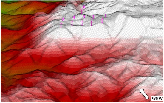
Figure 4.
Computational grid in the vicinity of the wind turbines.
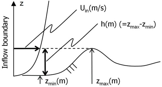
Figure 5.
Characteristic velocity and length scales (Uin and h).
4. Simulation Results and Discussion
Figure 6 shows the temporal changes of the non-dimensional scalar wind speed based on the three components of the wind velocity, Uscalar/Uin (=(u2 + v2 + w2)1/2/Uin), which were calculated at the hub heights (50.0 m above the ground surface, refer to Figure 3) of all wind turbines, WTs No. 1 to No. 6. In Figure 6, the horizontal axis indicates non-dimensional time (=T/(h/Uin)). For a hypothetical value of Uin = 5.0 m/s for the actual wind velocity, the duration of time on the horizontal axis is approximately 45.0 min. An examination of Figure 6 reveals that an anomalous flow phenomenon is generated in the vicinity of the wind turbines, that is, the trends of the temporal change of the non-dimensional scalar wind speed are almost the same at all turbines, WTs No. 1 to No. 6. The wave pattern in the trends changes by alternating between low velocities and high velocities. As discussed in detail below, this wave pattern changes periodically, suggesting that terrain-induced turbulence is generated due to the topographic irregularities in the vicinity of the wind turbines passing through the wind turbines. Therefore, it can be speculated that all wind turbines, WTs No. 1 to No. 6, were subject to the effect of terrain-induced turbulence which originated from topographic irregularities, on a regular basis. Although it happened to be the nacelle of WT No. 3 that fell to the ground at the time of the accident, it may be claimed that this accident was bound to happen at one of the wind turbines on the wind farm and that it would have been no surprise even if the nacelle of a different wind turbine had fallen to the ground. Note that, in post-accident inspections, cracks similar to those on WT No. 3 were detected on all the turbines except for WT No. 1.
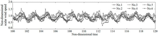
Figure 6.
Temporal changes of scalar wind speed at the hub height (50.0 m). Duration of time shown on the horizontal axis is approximately 45.0 min (for Uin = 5.0 m/s).
In a Reynolds-Averaged Navier–Stokes (RANS) model, the governing equations are Reynolds-Averaged (ensemble-averaged). Therefore, in a numerical wind simulation which uses a RANS model as the turbulence model, unsteady flow phenomena such as the one in Figure 6 cannot be simulated. Figure 7 shows the vertical profiles of streamwise wind velocities from all the wind turbine sites. These profiles were obtained by time-averaging (frame-averaging) the wind field over t = 100–120 in the non-dimensional time period shown in Figure 6. The results in this figure correspond to output from a RANS model. The variable z* on the vertical axis represents the height above the terrain surface (m), and the horizontal axis shows the normalized wind velocity. In regard to interpreting Figure 7, the following point should be noted. Figure 7 shows that large velocity shears are not present at any of the wind turbine sites at Taikoyama Wind Farm, i.e., WTs No. 1 to No. 6, although the mean streamwise wind velocities are locally enhanced due to topographic effects at all these sites. Judging from Figure 7 alone, one may tend to conclude that, from the point of view of wind conditions, serious problems are not expected to occur at any of the wind turbine sites WTs No. 1 to No. 6. Therefore, to examine the topographic effects on airflow at wind turbine sites, an examination that considers unsteady flow phenomena is crucial.
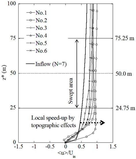
Figure 7.
Profile of mean streamwise wind velocity at each wind turbine site.
Henceforth, the discussion focuses on WT No. 3, the nacelle which fell to the ground in the present accident. Figure 8 shows the temporal changes of the angle of the wind on horizontal (yaw direction) and vertical cross-sections at the wind turbine hub height (50.0 m above the terrain surface), which are represented by the symbols ○ and □, respectively. The definitions of the two angles are also illustrated in Figure 8. The figure indicates that both angles change periodically with time in conjunction with the temporal changes of the non-dimensional scalar wind speed shown in Figure 6. An examination of the temporal change of the angle of the wind on the vertical cross-section, shown with the symbol □, reveals that wind blowing with angles close to ±25° occurs frequently. As indicated by points A (+28.5°) and B (+28.2°) in the figure, wind blowing upward with a large angle even exceeding 25° also occurs. Subsequently, the temporal change of the angle of the wind on the horizontal cross-section (yaw direction), shown with the symbol ○, is examined. As is the case for the angle of the wind on the vertical cross-section, wind blowing with angles of approximately ±25° occurs periodically. Figure 9 depicts the velocity vectors at WT No. 3 for the times indicated by points C (+28.1°, non-dimensional time: 106.0) and D (−40.4°, non-dimensional time: 107.5) in Figure 8. The corresponding vertical profiles of the streamwise wind velocity are shown in Figure 10. An examination of the side view of the vertical profile of the wind velocity vectors in Figure 9 and Figure 10 together leads to the following finding: within the swept area at both instances indicated by points C and D, the vertical profiles of the wind velocity do not deviate significantly from the vertical profile of the inflow wind velocity which follows a power law (N = 7) (heavy black line in Figure 10). In contrast, an examination of the rear view in Figure 9a shows that, at the time indicated by point C, the velocity vector rotates rapidly with height across the entire vertical profile. At the time indicated by point D, the velocity vector rotates gradually with height between the ground surface and the upper end of the swept area (Figure 9b). In this case, the rotation angle of the wind vector over the entire height is much smaller than that for the time indicated by point C.
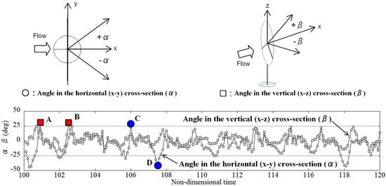
Figure 8.
Temporal changes of the angle of the wind on the horizontal (x–y) and the vertical (x–z) cross-sections at the hub height (50.0 m above the terrain surface) in the case of WT No.3. Duration of non-dimensional time on the horizontal axis is approximately 45.0 min (for Uin = 5.0 m/s).
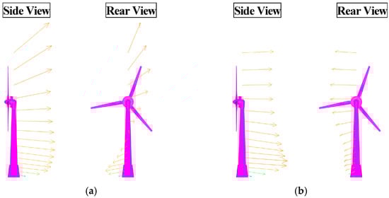
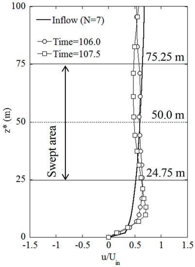
Figure 10.
Profiles of instantaneous streamwise wind velocity corresponding to Figure 9 (WT No.3).
The rotations of the wind velocity vector with height in the vertical profiles are attributable to the three-dimensional structure of the terrain-induced turbulence. It can be speculated that, as a result of the change of direction of the wind velocity vector with height, additional load was imposed in the vicinity of the base of the nacelle of WT No. 3, which connected the wind turbine tower and the blades. This condition, in turn, increased metal fatigue in the bolts on WT No. 3. The simulation results of the present study also show, across the height between the center of the wind turbine hub and the lower end of the swept area, the presence of multiple time periods characterized by large velocity shear, in which the vertical profile of wind velocity deviates significantly from that of the inflow wind velocity which follows a power law (N = 7) (not shown due to space limitations).
Figure 11 shows the vertical profiles of the standard deviations of the three components of the wind velocities evaluated from the wind field at each of the wind turbine sites. Specifically, the standard deviations were calculated with respect to the time-averaged (frame-averaged) values of wind velocities from the non-dimensional period t = 100–120 shown in Figure 6. The present study evaluates only the airflow fluctuations caused by terrain-induced turbulence which originates from the topographic irregularities and does not consider the fluctuating component of the inflow wind field (wind gusts). The values of the standard deviation of each component of the wind velocity are relatively large across the range of the swept area at all the wind turbine sites (Figure 11). It should also be noted that the values of the standard deviations of the x- and y-components (Figure 11a,b, respectively) are approximately the same. This result indicates that the temporal and spatial fluctuations of the airflow in the horizontal cross-section direction (yaw direction) are large at all of the wind turbine sites, as discussed for Figure 8 and Figure 9. It can be speculated that vertical and horizontal exciting forces were generated at and around the base of the nacelle of WT No. 3 due to the phenomena discussed above: (1) relatively large values of the standard deviation of the x-component of the wind velocity; (2) large values of the standard deviation of the z-component of the wind velocity; and (3) the standard deviation of the y-component of the wind velocity being approximately the same as that of the x-component. This leads to a possible explanation for the accident: the generated exciting forces damaged the bolts at the joint between the wind turbine body and the tower, which in turn would increase the exciting forces, resulting in the fatigue breakdown of the upper portion of the tower.
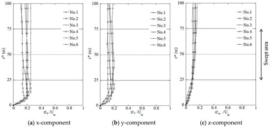
Figure 11.
Profiles of the standard deviations of the three components of the wind velocities at each of the wind turbine sites.
In the present study, an additional analysis was performed on the characteristics of the wind conditions at, and in the vicinity of, Taikoyama Wind Farm with the use of the surface level (10.0 m height above the ground surface) of the MSM (Meso Scale Model)—GPV (Grid Point Value) data distributed by the Japan Meteorological Agency (JMA). The analysis results reveal that southerly wind as well as westerly wind, which were described earlier, occurred frequently throughout the year for the three years from 2010 to 2012. As an example, Figure 12 shows analysis results of wind conditions in the area of Taikoyama Wind Farm during one of the three years, 2012. All the wind roses show that southerly is a frequently occurring wind direction.
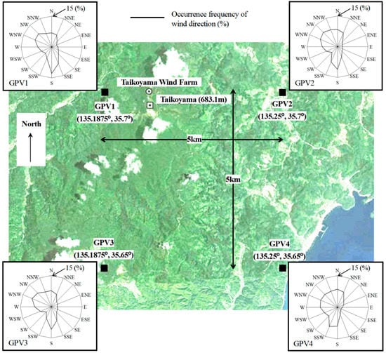
Figure 12.
Wind characteristics in the vicinity of Taikoyama Wind Farm based on MSM-S GPV data for 2012.
In light of the analysis results above, an unsteady, numerical wind diagnosis is conducted for southerly wind conditions using RIAM-COMPACT (Figure 13). This figure infers that all the wind turbines at Taikoyama Wind Farm are strongly affected by terrain-induced turbulence generated in the vicinity of the site marked by arrow A and that they operate immersed in airflow which fluctuates significantly in time both in wind speed and direction. Furthermore, the present diagnosis reveals the following additional concern: since WTs No. 1 to No. 5 are on a nearly straight line in the south-to-north direction, mutual interference between the wakes of the wind turbines (turbulence generated by the rotation of the blades of an upstream wind turbine affects downstream wind turbines, causing breakdown of the downstream wind turbines and/or reduction in electric power generated by the downstream turbines) may arise in the case of southerly wind appearing aloft over Taikoyama Wind Farm (see the conceptual figure in Figure 14).
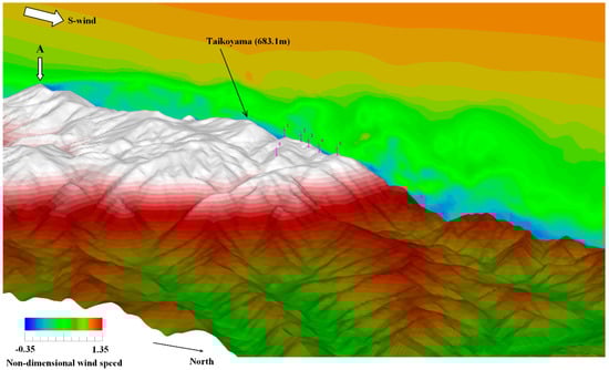
Figure 13.
Distribution of instantaneous streamwise velocity along the vertical cross-section.
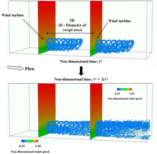
Figure 14.
Conceptual figure of wake interaction between two wind turbines by visualization of the Laplacian of the pressure field.
To summarize, the results of the numerical wind diagnosis infer that, in the case of southerly wind appearing over Taikoyama Wind Farm, additional load was imposed in the vicinity of the base of the nacelle, which connected the tower and the blades, due to the effects of both terrain-induced turbulence and turbulence caused by the rotation of the blades of the wind turbines (mutual interference between wakes of wind turbines). It can be speculated that the additional load, in turn, increased metal fatigue in the bolts at the base of the nacelle.
Finally, if a decision is to be made based on the results of the numerical wind simulation in the present study for “reconstruction” of the Taikoyama Wind Farm, the following course of action is worthy of consideration. All existing wind turbines are to be removed, a wind turbine model which is highly resistant to terrain-induced turbulence is to be selected, and one or two wind turbines of this model are to be constructed. During construction, it is preferable to make the towers as tall as possible. Since terrain-induced turbulence is generated and develops close to the ground surface fundamentally, the effect of terrain-induced turbulence on the wind turbine and supporting structure decreases dramatically with increasing tower height. Subsequently, a preliminary calculation is made on the economics for the case in which a single wind turbine is deployed on a 70.0 m tower (Figure 15). In this calculation, the time-series data of the wind velocity (10.0 m above the ground surface) at grid point GPV1, shown in Figure 12, from 2012 are used after being height-corrected. The results of the calculation reveal that the economics of the proposed future Taikoyama Wind Farm is typical in comparison to other wind farms in Japan. Therefore, it can be claimed that “reconstruction” of the Taikoyama Wind Farm is quite plausible if, in addition, appropriate maintenance and management are performed as laid out in the accident report [1].
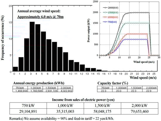
Figure 15.
Results of a preliminary calculation of economic feasibility for the case of one wind turbine (hub height = 70.0 m), based on the MSM-S GPV data from the location labeled GPV1 in Figure 12.
5. Conclusions
In the present study, unsteady numerical wind diagnoses were performed for Taikoyama Wind Farm with the use of an LES turbulence model. Based on the simulation results, with a focus on the effect of terrain-induced turbulence generated in the vicinity of the wind turbines, and from the viewpoint of numerical wind analysis, an examination was made of the Taikoyama Wind Farm nacelle separation accident, in which the nacelle of Wind Turbine (WT) No. 3 fell to the ground. The examination led to the following finding for all the wind turbine sites including WT No. 3: in the case of west-southwesterly wind conditions, the wind velocity shear deviated from the wind velocity shear in the vertical profile of the wind velocity that followed a power law (N = 7). For the same wind conditions, it was also found that large temporal changes in the angle of the wind on the hub height horizontal (yaw direction) cross-section occurred frequently at all wind turbine sites. Furthermore, an analysis of the airflow fluctuations caused by terrain-induced turbulence revealed additional characteristics of the wind across the heights of the swept area at all wind turbine sites. Specifically, the standard deviation of the streamwise (x) component of the wind velocity was relatively large, and that of the vertical (z) component was large. In addition, the values of the standard deviation of the spanwise (y) velocity component were approximately the same as those of the streamwise (x) velocity component. From the findings above, it can be speculated that the exciting force on WT No. 3 increased due to the effect of terrain-induced turbulence. The increased exciting force then imposed additional load in the vicinity of the base of the nacelle of the wind turbine, which connected the tower and blades, and thus increased metal fatigue in the bolts at the base of the nacelle. In the case of southerly wind conditions, it was found that the wind turbines were subject to, in addition to the effects of terrain-induced turbulence, the effects of turbulence caused by the rotation of blades of wind turbines (mutual interference between wakes of wind turbines).
Acknowledgments
This work was supported by JSPS KAKENHI Grant Number 17H02053. The author expresses appreciation to them.
Conflicts of Interest
The authors declare no conflict of interest.
References
- The Report of Wind Turbine Nacelle Separation Accident in the Taikoyama Wind Farm, Kyoto Prefecture, Japan. Available online: http://www.meti.go.jp/committee/sankoushin/hoan/denryoku_anzen/newenergy_hatsuden_wg/pdf/001_03_02.pdf (accessed on 26 December 2013). (In Japanese).
- Liu, Z.Q.; Ishihara, T. Numerical study of turbulent flow over complex topography by LES model. In Proceedings of the Sixth International Symposium on Computational Wind Engineering, Hamburg, Germany, 8–12 June 2014. [Google Scholar]
- Uchida, T.; Ohya, Y. Micro-Siting technique for wind turbine generators by using large-eddy simulation. J. Wind Eng. Ind. Aerodyn. 2008, 96, 2121–2138. [Google Scholar] [CrossRef]
- Uchida, T.; Maruyama, T.; Ohya, Y. New evaluation technique for WTG design wind speed using a CFD-model-based unsteady flow simulation with wind direction changes. Model. Simul. Eng. 2011, 2011, 941870. [Google Scholar] [CrossRef]
- Uchida, T.; Ohya, Y. Latest developments in numerical wind synopsis prediction using the RIAM-COMPACT CFD model. Energies 2011, 4, 458–474. [Google Scholar] [CrossRef]
- Uchida, T. High-Resolution LES of terrain-induced turbulence around wind turbine generators by using turbulent inflow boundary conditions. Open J. Fluid Dyn. 2017, 7, 511–524. [Google Scholar] [CrossRef]
- Uchida, T. Large-Eddy simulation and wind tunnel experiment of airflow over Bolund Hill. Open J. Fluid Dyn. 2017, 8, 30–43. [Google Scholar] [CrossRef]
- Uchida, T. High-resolution micro-siting technique for large scale wind farm outside of japan using LES turbulence model. Energy Power Eng. 2017, 9, 802–813. [Google Scholar] [CrossRef]
- Uchida, T. CFD Prediction of the airflow at a large-scale wind farm above a steep, three-dimensional escarpment. Energy Power Eng. 2017, 9, 829–842. [Google Scholar] [CrossRef]
- Kim, J.; Moin, P. Application of a fractional-step method to incompressible Navier-Stokes equations. J. Comput. Phys. 1985, 59, 308–332. [Google Scholar] [CrossRef]
- Kajishima, T.; Taira, K. Computational Fluid Dynamics: Incompressible Turbulent Flows; Springer: New York, NY, USA, 2016; ISBN 978-3319453026. [Google Scholar]
- Kawamura, T.; Takami, H.; Kuwahara, K. Computation of high reynolds number flow around a circular cylinder with surface roughness. Fluid Dyn. Res. 1986, 1, 145–162. [Google Scholar] [CrossRef]
- Smagorinsky, J. General Circulation Experiments with the Primitive Equations, Part 1, Basic Experiments. Mon. Weather Rev. 1963, 91, 99–164. [Google Scholar] [CrossRef]
© 2018 by the author. Licensee MDPI, Basel, Switzerland. This article is an open access article distributed under the terms and conditions of the Creative Commons Attribution (CC BY) license (http://creativecommons.org/licenses/by/4.0/).