Energy Management Strategy for Hybrid Electric Vehicle Based on Driving Condition Identification Using KGA-Means

1
State Key Laboratory of Mechanical Transmissions, School of Automotive Engineering, Chongqing University, Chongqing 400044, China
2
Chongqing Changan Automobile Co., Ltd., Chongqing 400023, China
*
Author to whom correspondence should be addressed.
Energies 2018, 11(6), 1531; https://doi.org/10.3390/en11061531
Submission received: 4 May 2018
/
Revised: 28 May 2018
/
Accepted: 8 June 2018
/
Published: 12 June 2018
Abstract
:In order to solve the problem related to adaptive energy management strategies based on driving condition identification being difficult to be applied to a real hybrid electric vehicle (HEV) controller, this paper proposes an energy management strategy by combining the driving condition identification algorithm based on genetic optimized K-means clustering algorithm (KGA-means), and the equivalent consumption minimization strategy (ECMS). The simulation results show that compared with ECMS, the energy management strategy proposed in this article drives the engine working point closer to the best efficiency curve, and smooths out the state of charge (SOC) change and better maintains the SOC in a highly efficient area. As a result, the vehicle fuel consumption reduces by 6.84%.
1. Introduction
An hybrid electric vehicle (HEV) power system consists of multiple power sources. An appropriate energy management strategy coordinates the power system components, and achieves a reasonable distribution of the demanded power between multiple power sources. As a result, improved fuel economy can be attained along with satisfactory dynamic performance. The recently proposed adaptive energy management strategies present superior performance, but they are difficult to be implemented in real HEVs. Therefore, research on a real-time energy management strategy based on driving condition identification is of great practical value and theoretical significance.
So far, several adaptive energy management strategies have been proposed in the literature. Sun et al. [1] used a radial basis function neural network to predict driving conditions, and applied minimal values to the predicted result. As such, the coordinated control of a hybrid power system was conducted, and its fuel economy was improved. Wang et al. [2] analyzed the relationship between the characteristic parameters and driving condition categories, and the relationship between the driving condition identification periods and predicted periods of driving condition identification. On this basis, the most sensible driving condition identification period and predicted periods of driving condition identification were selected. Then, the learning vector quantization (LVQ) neural network was employed to identify driving conditions, and the equivalent consumption minimization strategy (ECMS) was utilized to achieve the fuel economy. Zheng et al. [3] established a prediction model based on global positioning system (GPS) and geographic information system (GIS) in which the battery state of charge (SOC) was used as a state variable, the power output of the battery was the control variable, fuel consumption was the optimization goal, and the minimum value principle was used to optimize the vehicle power distribution according to the predicted future road information. Guardiola et al. [4] analyzed the impact of driving behavior on the energy management strategy of HEVs, established a Markov forecast model to predict driver behavior, and adjusted the equivalent fuel coefficient in combination with ECMS to achieve adaptive power distribution. Musardo [5] proposed an adaptive energy management strategy that was used to recognize driving conditions and driving patterns based on GPS and previous driving conditions, and then adjusted the equivalent fuel coefficient based on the predicted results to achieve the real-time adjustment of torque distribution. Qin et al. [6] applied Euclidean proximity to identify the driving conditions and used particle swarm optimization (PSO) to optimize the energy management parameters under different driving conditions. Yang et al. [7] selected six kinds of circulating road-driving conditions as standard driving conditions, and used the limit learning machine to identify the driving conditions. Then, the minimum value principle was applied to obtain an off-line optimized parameter database corresponding to a number of standard driving conditions, which were combined with the driving condition identification results to update the control strategy parameters in real-time. Thus, the optimization of a plug-in hybrid electric vehicle (PHEV) energy control strategy based on driving condition identification was achieved. The above driving condition identification algorithms presented some certain deficiencies. The neural network-based methods required a certain number of a priori input and output data. Usually, the driving conditions were used as the input data, and the types of driving conditions were the output data. However, the number of driving conditions in clear driving condition categories is so low that no sufficient input and output data could be provided for neural network training. This jeopardized the identification accuracy of the neural network and affected the performance of energy management strategies. When fuzzy mathematics is used to identify driving conditions, the selection of membership functions in fuzzy mathematics is highly empirical. The identification accuracy is sensitive to membership function tuning, and the tuning itself is very time-consuming.
In light of the existing HEV energy management strategies, this paper proposes a single-motor HEV energy management strategy based on driving condition identification, aiming to improve the HEV fuel economy. Firstly, four typical cycle driving conditions are selected, and the driving condition identification characteristic parameters are optimized to reduce driving condition identification complexity. Secondly, the K-means clustering algorithm (KGA-means) is applied to a random driving condition identification. The existing driving condition identification approaches cannot be directly implemented in practice due to the large computation load. With the proposed method, the real-time identification of driving conditions is realized. Thirdly, based on the ECMS, the relationship between different equivalent fuel coefficients and fuel consumption under four typical driving conditions is obtained. Then, the optimal vehicle power distribution under different typical driving conditions is achieved. Under the current type of driving conditions, the demanded power can be reasonably distributed so as to improve the fuel consumption.
The remainder of this paper is divided into six sections. In the next section, HEV power transmission system structure and parameters are illustrated. The third section presents the optimization of driving condition identification characteristic parameters. An energy management strategy based on driving condition identification using KGA-means is described in the fourth section. In the fifth section, the materials and methods are illustrated. The paper presents conclusions in the sixth section.
2. HEV Power Transmission System Structure and Parameters
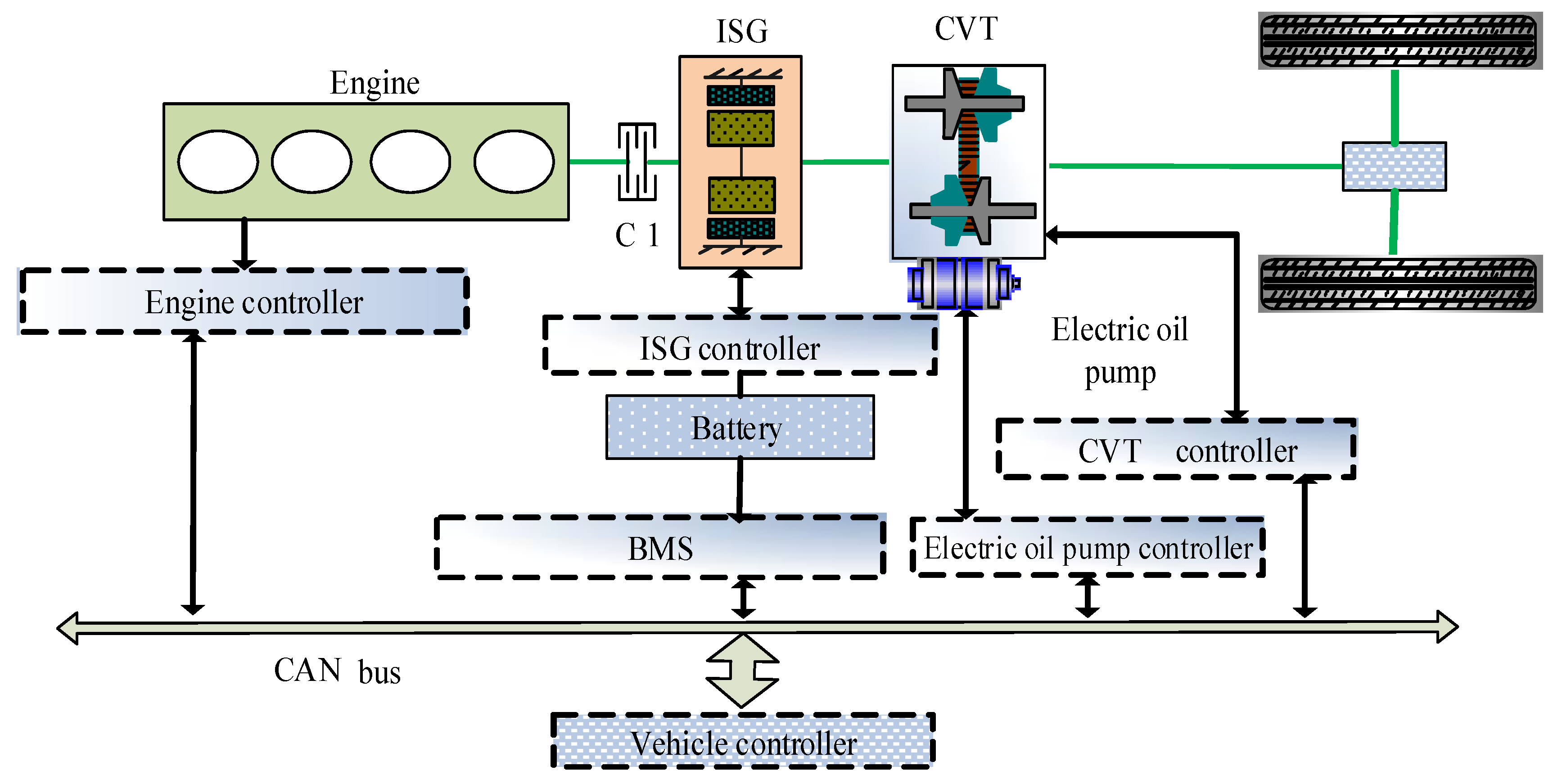
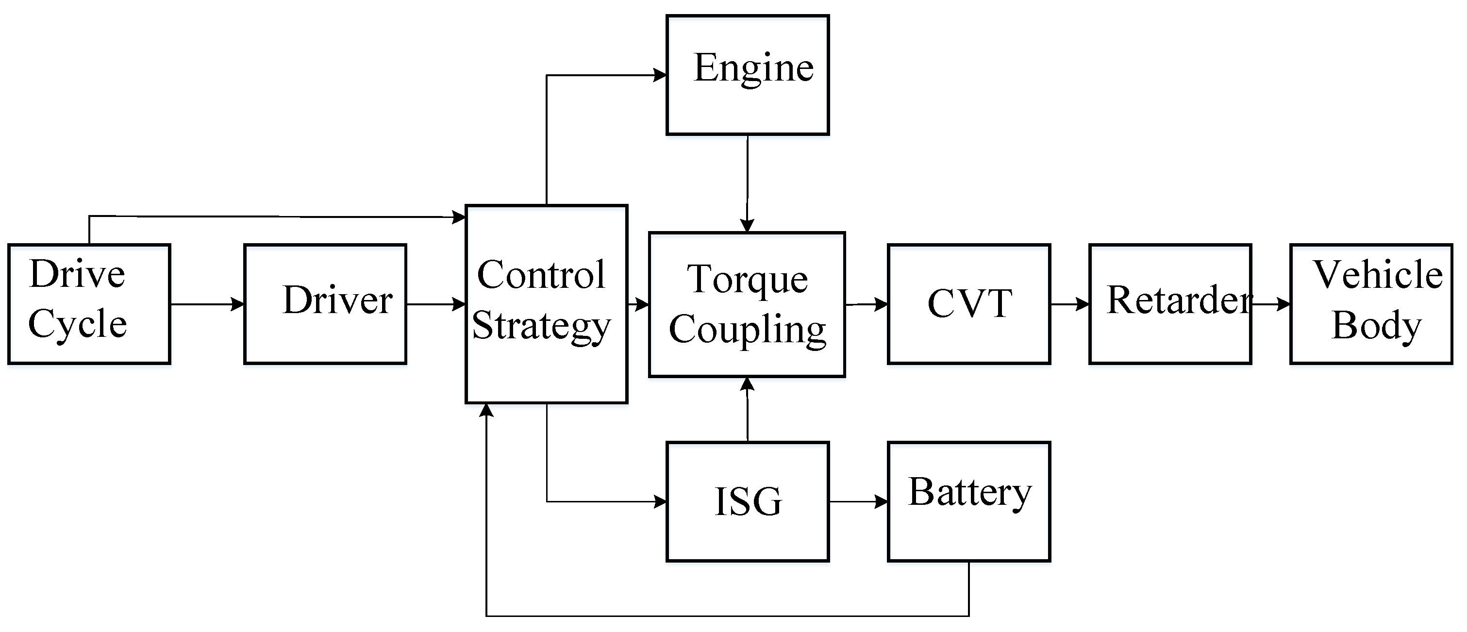
The HEV structure considered in this paper is shown in Figure 1. The main components include the engine, an integrated starter and generator (ISG) [8], a wet multi-disc clutch (C1), a continuously variable transmission (CVT), a battery pack, a battery management system (BMS), and final drive. The vehicle controller switches the working modes by controlling the wet multi-plate clutch C1, ISG, CVT, and engine. Through the controller area network (CAN) bus, the communication between the engine controller, motor controller, BMS, and CVT controller is realized. Based on this communication, the vehicle controller monitors the vehicle operating status and controls the operating modes, torques, and speeds of the ISG and engine. The main parameters of this HEV power system are given in Table 1.
3. Optimization of Driving Condition Identification Characteristic Parameters
An optimization of the number of driving condition characteristic parameters can reduce the computation load and improve the driving condition identification efficiency, which provides both theoretical significance and practical value.
3.1. Selection of Four Typical Driving Conditions
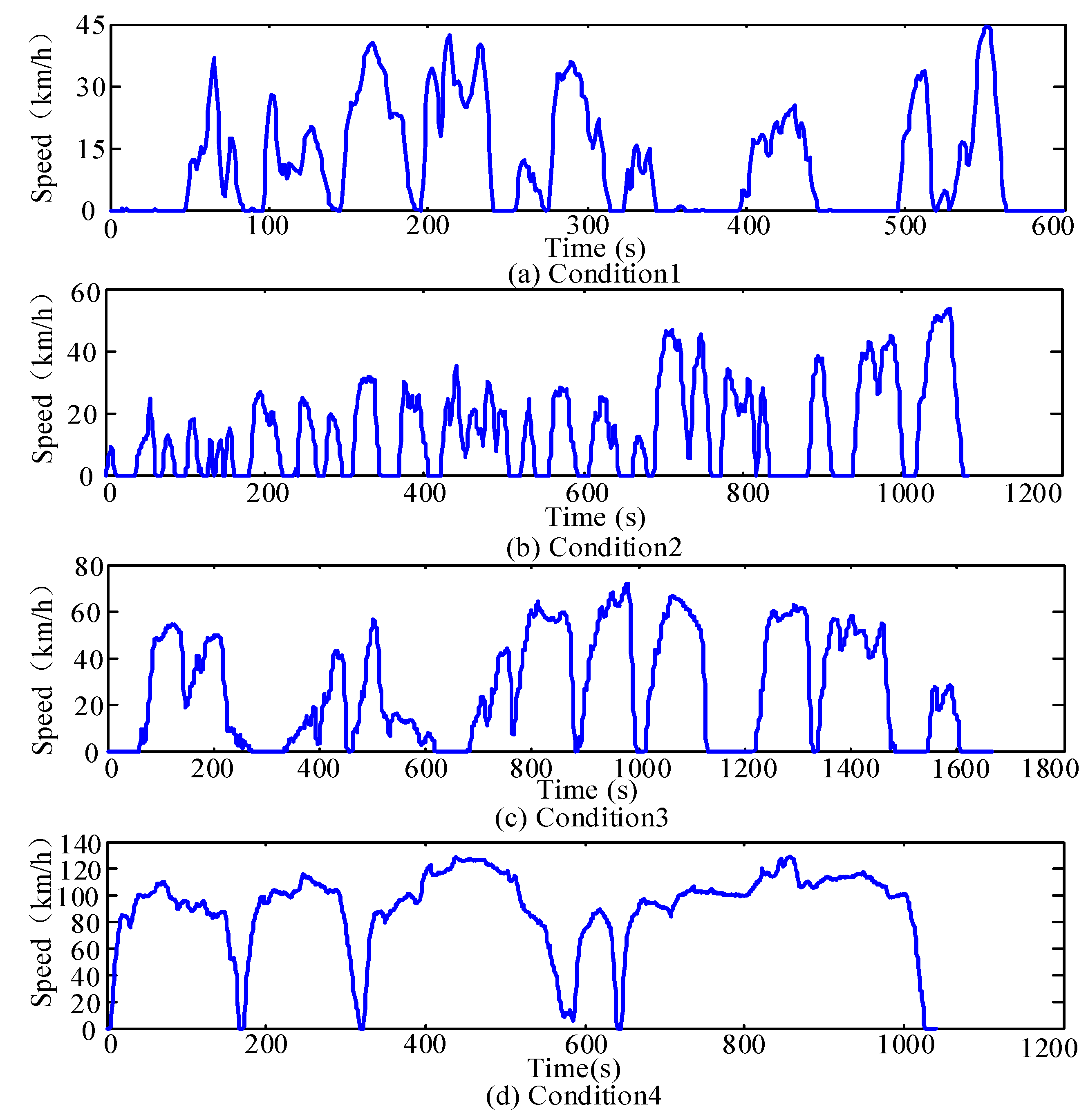
Based on the driving area and the traffic driving conditions reflected in the driving condition data, the driving conditions fall into four categories: congested driving conditions, urban driving conditions, suburban driving conditions, and highway driving conditions [9]. As such, four typical driving conditions are selected for driving condition identification: Condition 1 represents the congestion condition, which mainly occurs downtown, and features traffic jams and frequent stop-and-go movement. Condition 2 represents the urban condition, with increased speed compared with condition 1, and a similar stop-and-go situation. Condition 3 is the suburban condition, which mainly takes place on suburban or rural roads, with medium vehicle speed. Condition 4 is the highway condition, which features high speeds and smooth driving. All four typical cycles are shown in Figure 2.
3.2. Selection and Pretreatment of Basic Driving Condition Data
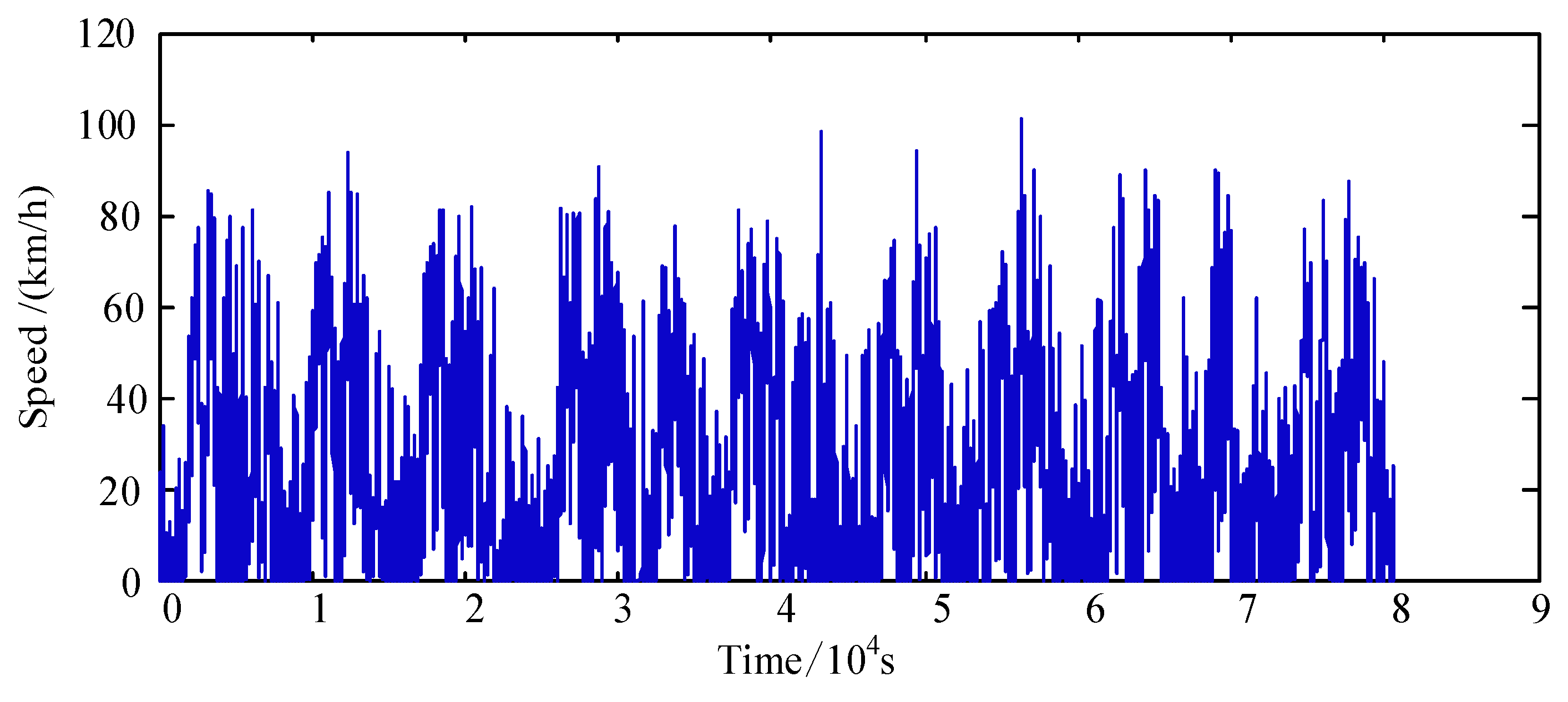
The basic driving data used in this paper was collected in a major city in China. The experimental route has covered highways, suburbs, residential areas, and urban centers. The experiment time includes rush hour, weekend, and different time spans on the same day, in order to acquire sufficient samples and guarantee data reliability. In one month, 30 groups of driving condition data were acquired, with a sampling period of 0.1 s. The pretreated basic driving condition data is given in Figure 3. The basic driving condition data includes four driving conditions: congested driving conditions, urban working driving conditions, suburban working driving conditions, and highway driving conditions.
According to the results reported in reference [10], the identification period is set to 150 s, and the prediction period is set to 3 s in this paper. Then, the driving data is divided into segments for every 150 s, and 14 commonly used driving condition characteristic parameters are extracted from the segments. These characteristic parameters are: average speed vmean, maximum speed vmax, average acceleration amean, average positive acceleration ameana, average negative acceleration ameand, idle time ratio (percentage of the total time to the entire cycle time) ridel, cruise time ratio rdrive, maximum acceleration amax, minimum acceleration amin, travel distance s, speed variance vvar, acceleration variance avar, speed square sum vspa, and acceleration square sum aspa.
3.3. Optimization of Characteristic Parameters
In the literature, two methods are commonly employed to optimize the characteristic parameters of driving conditions. One is to analyze the influence of characteristic parameters on vehicle performance (e.g., fuel economy), and the other is to analyze the ability of characteristic parameters to characterize driving conditions [11,12], neither of which is able to achieve optimal representative characteristic parameters by itself. On the other hand, certain characteristic parameters can well reflect the fuel economy or have strong a ability to characterize driving conditions. However, if a parameter candidate is very insensitive to driving conditions, then it is not considered a desirable characteristic parameter for driving condition identification. Therefore, it is necessary to optimize the characteristic parameters by taking into account: (1) the relationship between characteristic parameters and fuel consumption (the effect of characteristic parameters on fuel economy); (2) the correlation between various characteristic parameters (the ability of characteristic parameters to characterize the features of driving conditions); and (3) the sensitivity of characteristic parameters to driving conditions. The detailed optimization process is as follows:
Step 1: Analyze the ability of each parameter to characterize driving conditions through the correlation between the characteristic parameters. The characteristic parameters with correlation coefficient (defined by Equation (1)) above 0.8 can be replaced with each other.
Step 2: Analyze the correlation between the characteristic parameters and the fuel consumption to determine the influence of the characteristic parameters on fuel economy. The characteristic parameters are considered to be related to fuel economy only when the correlation coefficient is above 0.2.
Step 3: Analyze the change and change rate of each characteristic parameter. The coefficients are considered to meet the requirements when they are above 0.2.
The correlation coefficient is defined as Equation (1):
where xi and yi are the i-th sample of the two sample data with sample size n, and and are the average value of the two sample data, respectively.
The sensitivity of characteristic parameters to driving conditions is determined by R1 and R2, where R1 reflects the variation range of the characteristic parameters, and R2 represents the variation speed. The mathematical expressions for R1 and R2 are given by:
where xt is the value of the t-th sample in the database with sample size n, and f0.98 and f0.02 are the argument’s values of some cumulative distribution function at function values of 0.98 and 0.02, respectively. This paper selects f0.98 and f0.02 to eliminate the influence of singularities in the sample on the test results, thereby improving test accuracy.
The correlation coefficients between characteristic parameters are shown in Table 2. The correlation coefficients between characteristic parameters and the fuel consumption of traditional vehicles and HEVs are shown in Table 3. The sensitivity coefficients R1 and R2 are shown in Table 4. After conducting the optimization process outlined by the above three steps, vmean and rdrive are selected as the representative characteristic parameters.
4. Energy Management Strategy Based on Driving Condition Identification Using KGA-Means
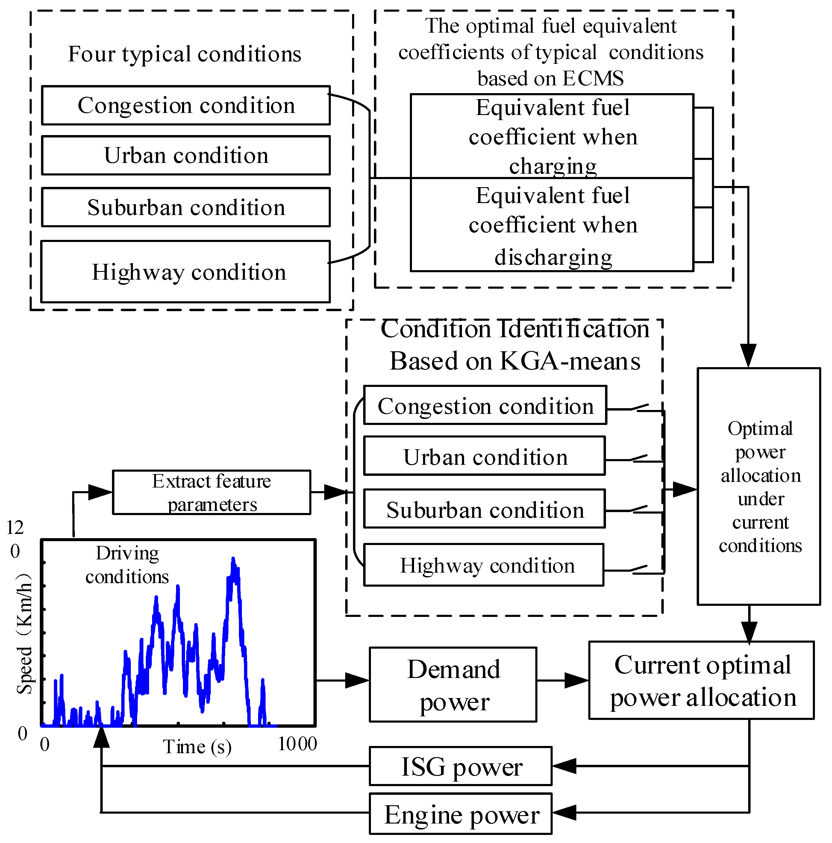
The energy management strategy employed in this study combines the ECMS with driving condition identification using KGA-means. This strategy can be divided into three steps:
Step 1: Extract characteristic parameters from the basic driving condition data, apply the KGA-means to classify the driving condition types, and obtain the final clustering center.
Step 2: Extract characteristic parameters from a random driving condition, and perform driving condition identification to obtain the category of the current driving condition.
Step 3: Apply the ECMS to obtain the optimal equivalent fuel coefficients corresponding to the four typical driving conditions, so that the optimal power distribution under the typical driving conditions is obtained. Then, carry out the optimal power distribution for the current driving condition category, and improve the fuel economy.
In summary, firstly, to identify a random driving condition, the optimized characteristic parameters are employed in the driving condition identification algorithm based on KGA-means. Secondly, the ECMS is applied to obtain the relationship between different equivalent fuel coefficients and fuel consumption under four typical driving conditions. On this basis, the optimal distribution of demanded power for different types of driving conditions is obtained. Finally, combining driving condition identification based on KGA-means with optimal power distribution of different driving conditions, a real-time energy management strategy for driving condition identification is obtained. This process is schematic shown in Figure 4.
4.1. Genetic Optimization of K-Means Clustering Center for Driving Condition Identification
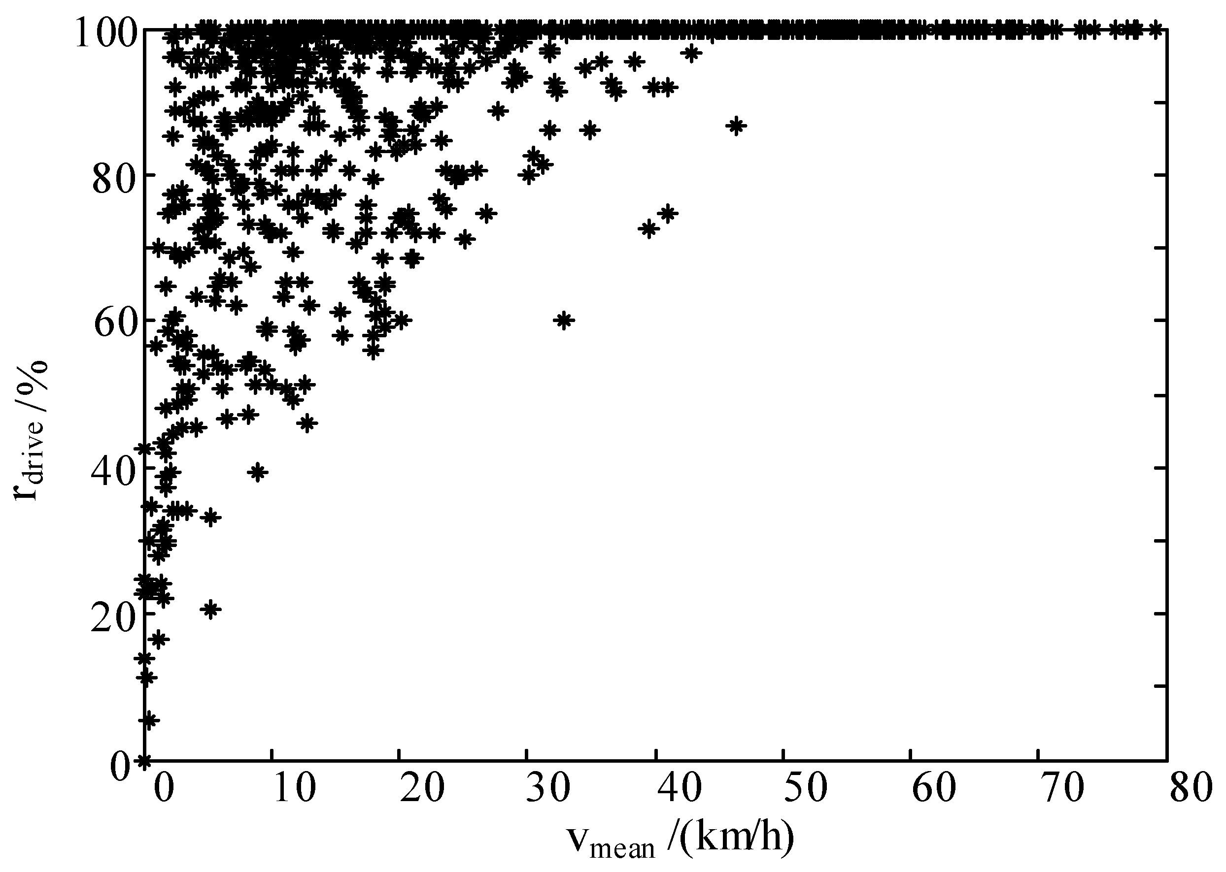
The specific process of clustering center genetic optimization consists of the following two steps. Firstly, select the basic driving condition data and divide it into driving condition segments. Then, extract the characteristic parameters to plot the driving condition fragment two-dimensional scatter plot. Secondly, apply a genetic algorithm to optimize the initial clustering center and obtain the genetically optimized initial clustering center.
The basic driving condition data is divided into driving condition segments with a length of 150 s. Then, vmean and rdrive are extracted to draw a two-dimensional scatter plot, as shown in Figure 5. The genetic optimization algorithm is employed to optimize the initial K-means clustering center, and the K-means clustering analysis is performed on the basic driving condition data to obtain the final clustering center. The basic driving condition data clustering analysis results are shown in Figure 6. In the figure, the basic driving condition data is divided into four clusters. Cluster 1 represents the congestion condition, cluster 2 represents the urban condition, cluster 3 represents the suburban condition, and cluster 4 represents the highway condition The final cluster centers are located at (3.8846, 34.2299), (11.6812, 70.5417), (16.5679, 96.4057), and (50.4290, 99.7460).
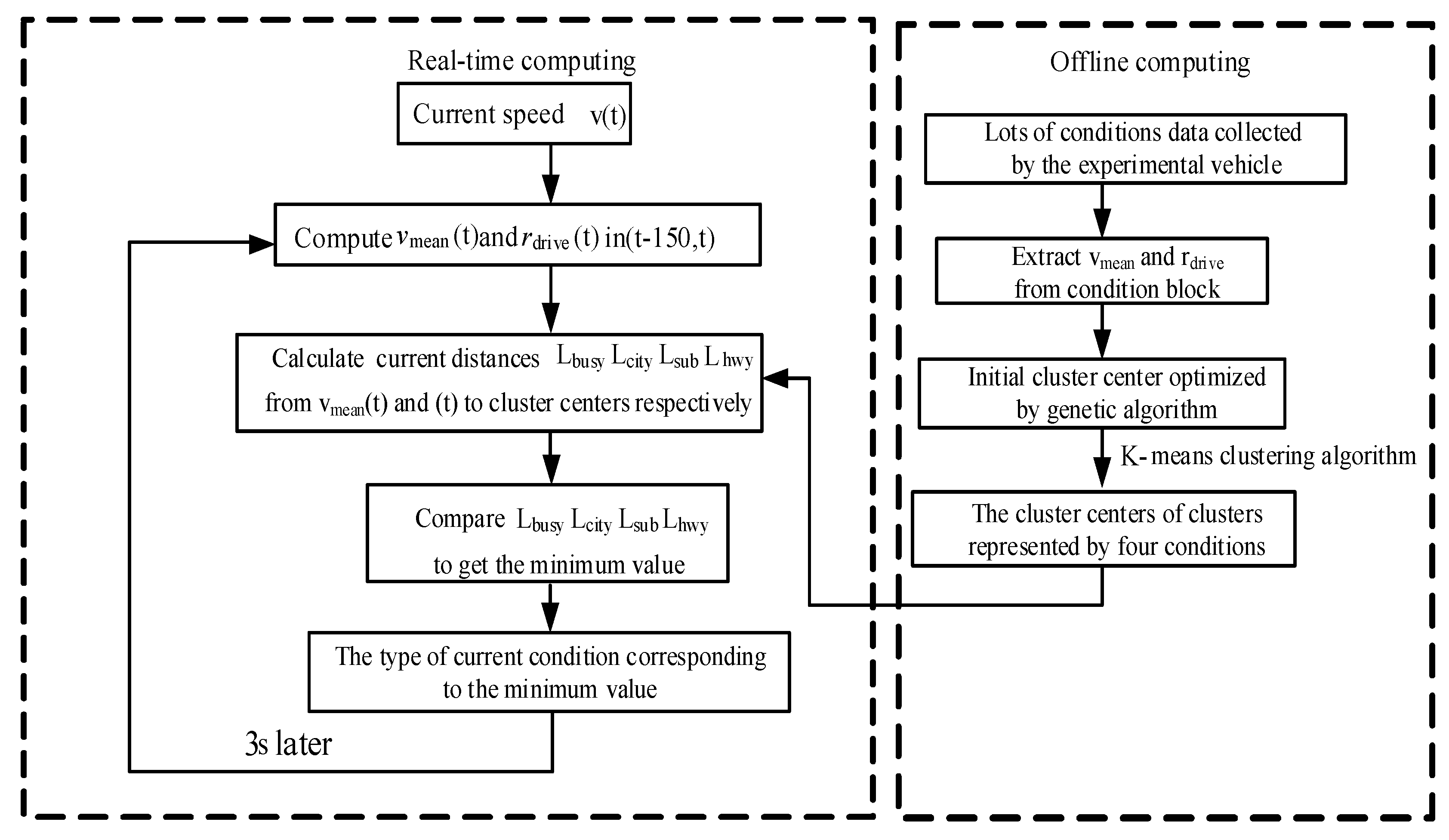
4.2. Driving Driving Condition Identification Algorithm Based on KGA-Means
The flow chart of the driving condition identification algorithm based on KGA-means is shown in Figure 7. The experimental vehicle has collected a large amount of driving condition data, which is divided into driving condition segments to extract vmean and rdrive. The initial clustering center of the K-means clustering algorithm is optimized by the genetic algorithm; then, the clustering center of different clusters is obtained by the K-means clustering algorithm. The K-means clustering algorithm is applied to divide the driving condition data into four different types. Assume that the current time is t and the vehicle speed at the current moment is v(t); calculate vmean(t) and rdrive(t) in (t-150, t) in real time. Then, based on the calculated vmean(t) and rdrive(t), the four distances of cluster centers, Lbusy, Lcity, Lsub, and Lhwy, corresponding to congestion condition, urban condition, suburban condition, and highway condition, can be computed. The types of driving conditions after 3 s correspond to the nearest cluster center.
4.3. Optimal Distribution of Demanded Power under Typical Cycle Driving Conditions
4.3.1. ECMS
This strategy minimizes the total energy consumption by optimizing the power distribution between the engine and the ISG under various instantaneous driving conditions [13]. That is, at each time t, the sum of the engine actual fuel consumption and the ISG equivalent fuel consumption is minimized. This is mathematically expressed by Equation (4):
where is the total equivalent fuel consumption, denotes the engine actual fuel consumption, and represents the ISG equivalent fuel consumption. First, can be obtained by means of engine steady-state model interpolation, and the formula for calculating is as follows:
where k = 0.5{1 + sign [Pm(t)]}, Pm(t) is the current ISG power, Rlhv is the gasoline mass calorific value constant, and λequ is the equivalent fuel coefficient given by:
where λchar and λdis are the equivalent fuel coefficients of the ISG for battery charging and discharging, respectively, , and represent the average efficiencies of ISG for battery charging and discharging under the current driving condition and power distribution mode, and and denote the average efficiencies of the engine and ISG under the current driving condition and power distribution mode.
The objective function and constraints [5] for this optimization are expressed as follows:
where Preq(t) is the current demanded power, Pe(t) is the current engine power, Pe_min and Pe_max are the minimum and maximum engine power, respectively, Pm_min and Pm_max are the minimum and maximum ISG power, respectively, and SOCL and SOCH are the upper and lower limits of the battery SOC maintenance range, respectively.
Within the constraints of the objective function, the power operating points of the engine and ISG that satisfy the power equilibrium equation are calculated, based on the demanded power at the time of interest. Then, the measured fuel consumption rate map of the engine and the equivalent fuel consumption rate model of the motor are employed to calculate the corresponding fuel consumption rate by means of interpolation [14]. The minimum fuel consumption rate is obtained by ECMS, and the operating points of the engine and ISG corresponding to the minimum fuel consumption rate are the best outputs at the current time.
4.3.2. Estimation of Optimal Fuel Equivalent Coefficient in Four Typical Cycle Driving Conditions
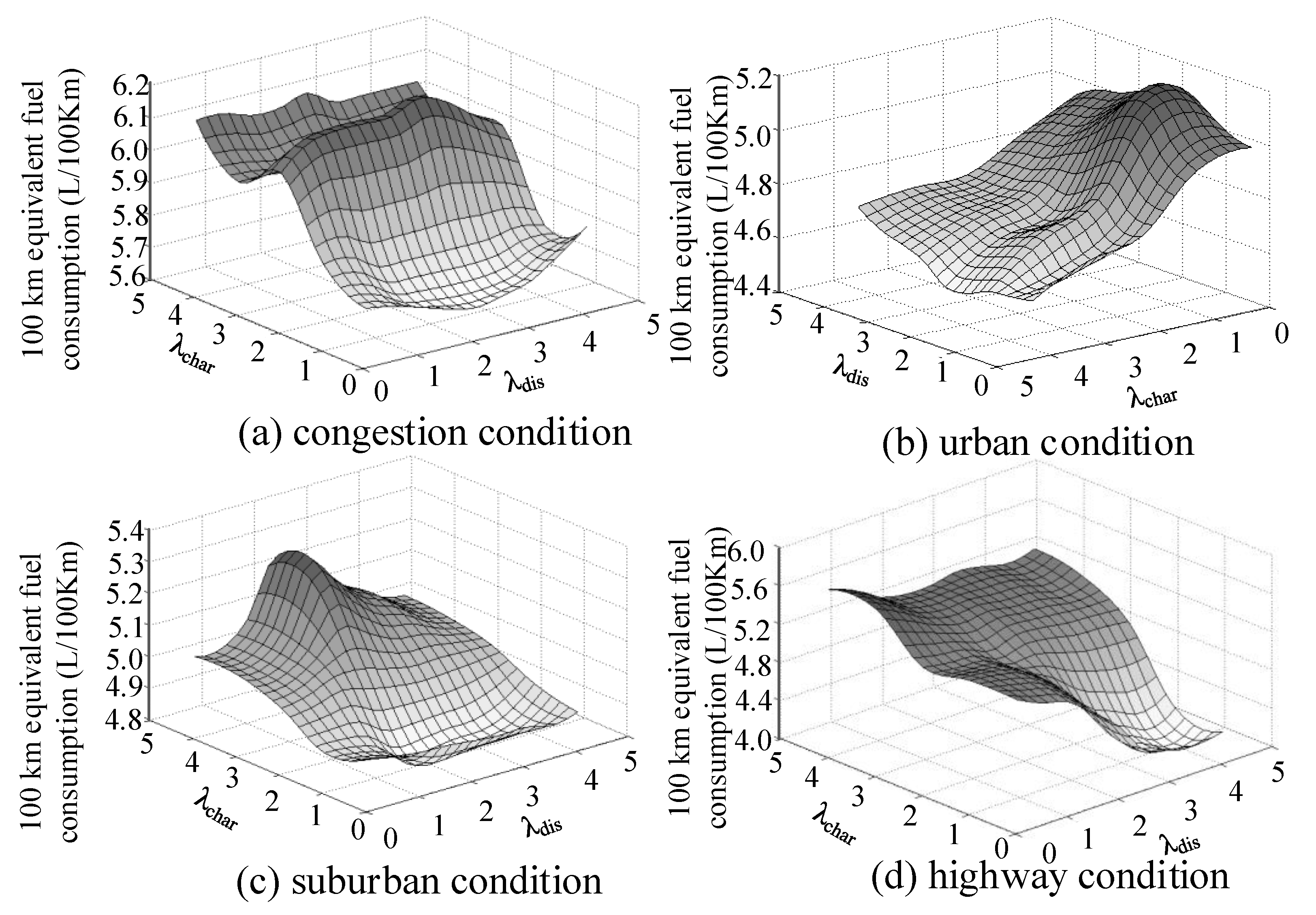
The demanded power of the HEV under four typical driving conditions is distributed according to the ECMS, and the fuel consumption rates under different equivalent fuel ratios are obtained by the finite-step-exhaust-exit method. The range of the equivalent fuel coefficient is determined by considering the engine operating points, engine critical points, and motor switching in the energy management strategy [15]. The relationship between the equivalent fuel consumption and the equivalent fuel coefficient under four typical driving conditions is shown in Figure 8:
4.3.3. Optimal Distribution of Demanded Power under Four Typical Driving Conditions
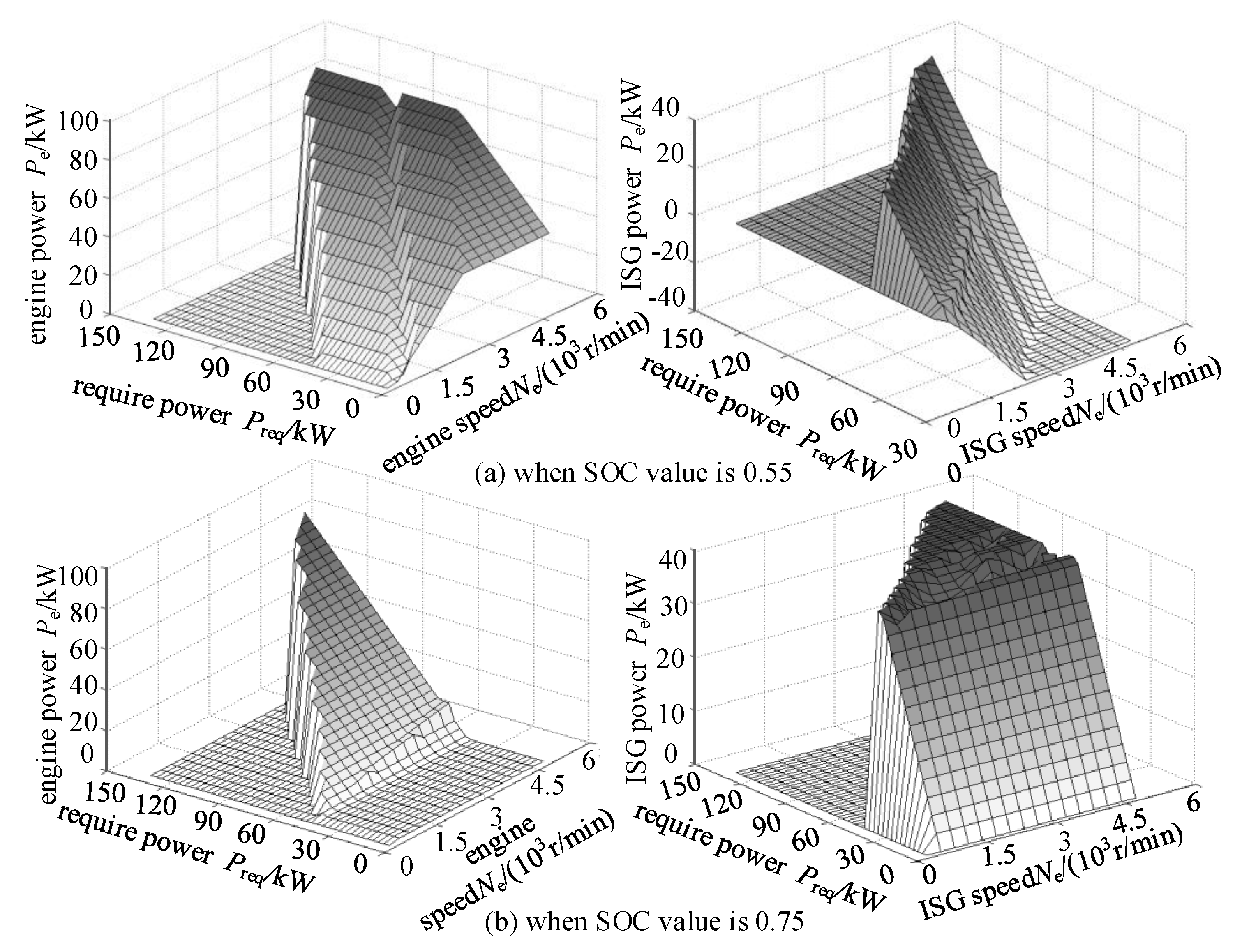
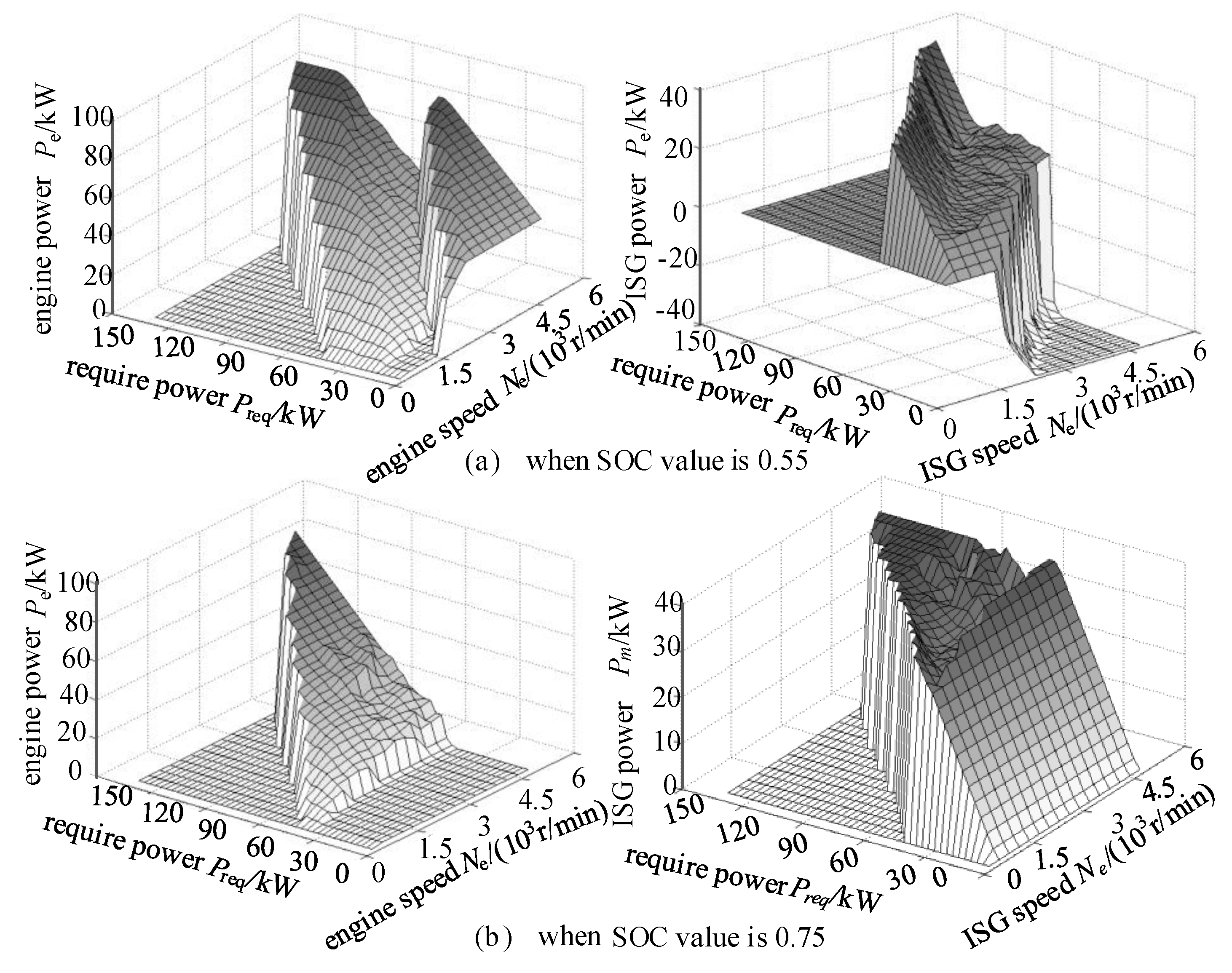
The optimal power distribution corresponds to the optimal equivalent fuel coefficient, and it is related to the current SOC and engine speed. Due to the page limit, this paper only lists the optimum distributions of the demanded power with 0.55 and 0.75 SOC values under urban and highway conditions, as shown in Figure 9 and Figure 10. These figures demonstrate the distribution differences with the same SOC values under different driving conditions, as well as the differences with different SOC values under the same driving condition.
It is also shown in Figure 9 and Figure 10 that the ISG provides more power when the HEV is in the urban condition than in the highway condition. When the SOC value is 0.75, the demanded power is preferentially provided by the ISG, and when the SOC value is 0.55, the battery is charged. The energy management strategy proposed in this article improves the fuel efficiency of the HEV, because the power distribution between the engine and the ISG is coordinated according to the optimal distribution of the demanded power under the identified current driving condition.
5. Materials and Methods
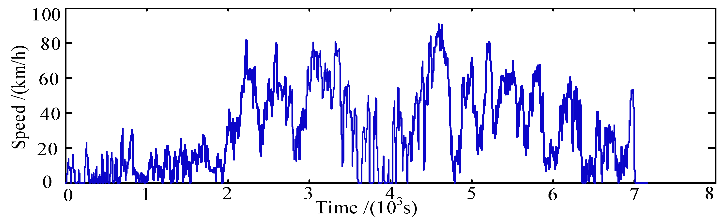
In order to verify the proposed energy management strategy, a simulation model of the entire vehicle is constructed using MATLAB/Simulink (MathWorks, Natick, MA, USA), as shown in Figure 11. The effectiveness of the proposed energy management strategy is verified with a random driving condition drawn in Figure 12.
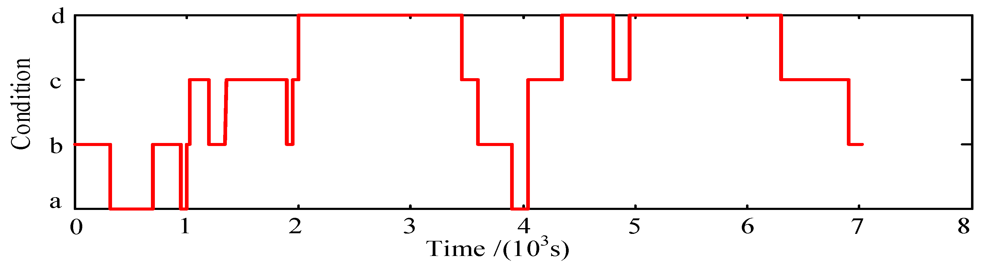
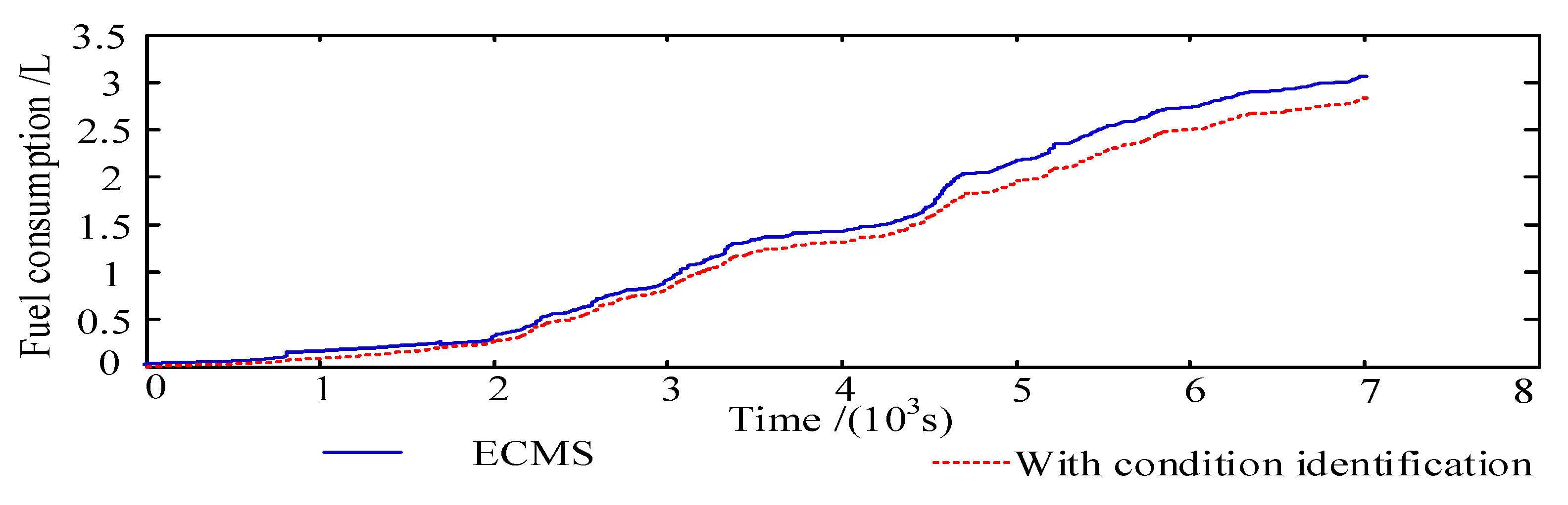
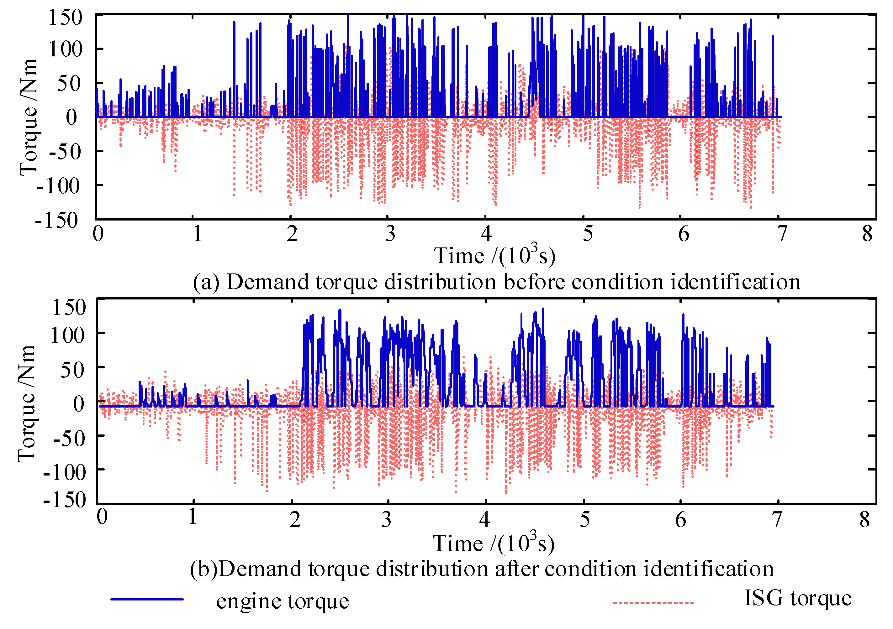
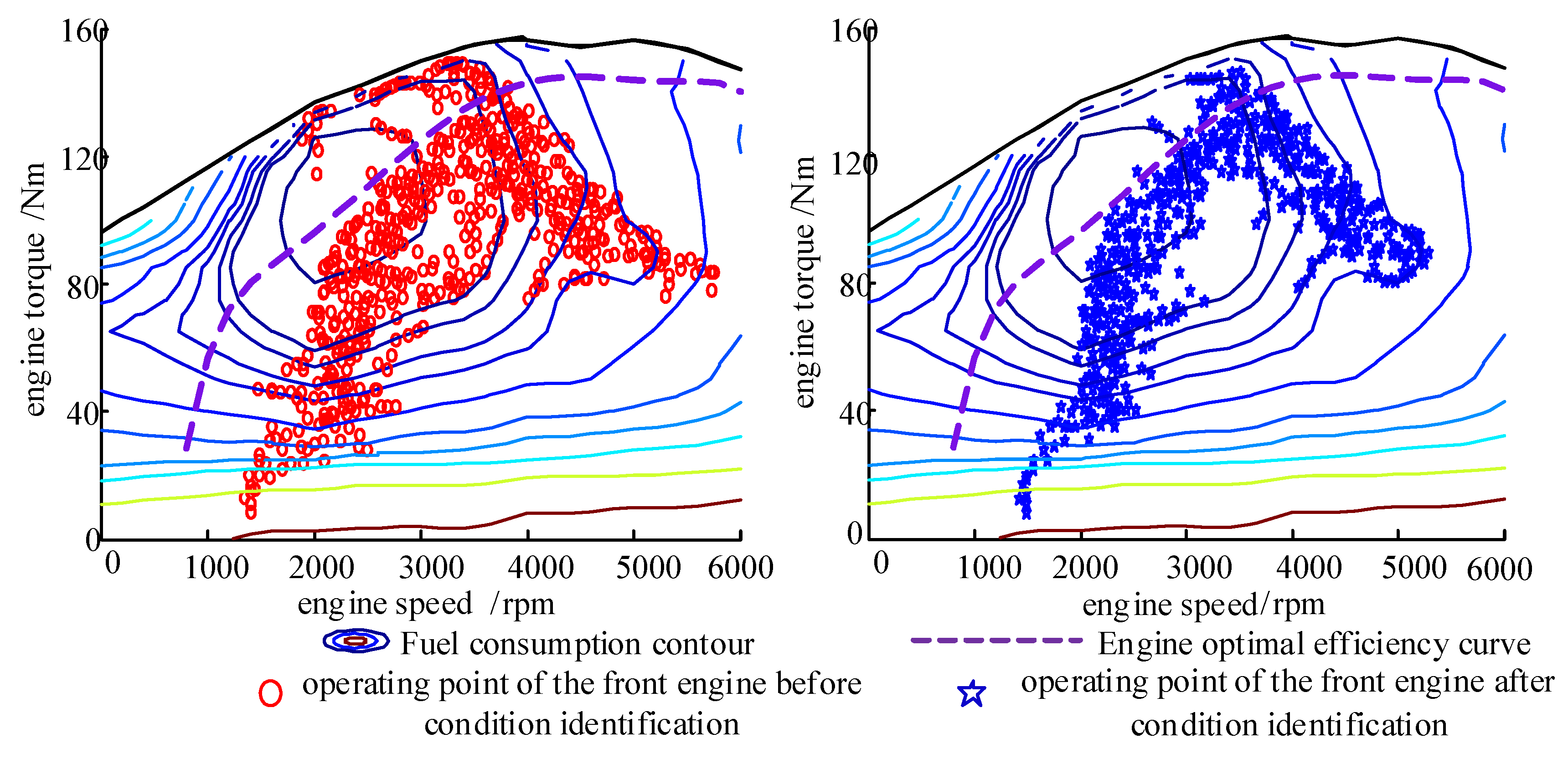
In this section, the ECMS without driving condition identification is compared with the proposed energy management strategy. The optimal equivalent fuel coefficients λchar and λdis resulting from the ECMS are 2.8 and 2.6, which are obtained under the simulated random driving condition. The identification results of the random driving conditions are shown in Figure 13, where a, b, c, and d represent the congestion condition, urban condition, suburban condition, and highway condition, respectively. The fuel consumptions resulting from the two energy management strategies are shown in Figure 14. The demanded torque distribution is expressed in Figure 15. The engine operating point distribution is shown in Figure 16. The battery SOC variation curves are plotted in Figure 17.
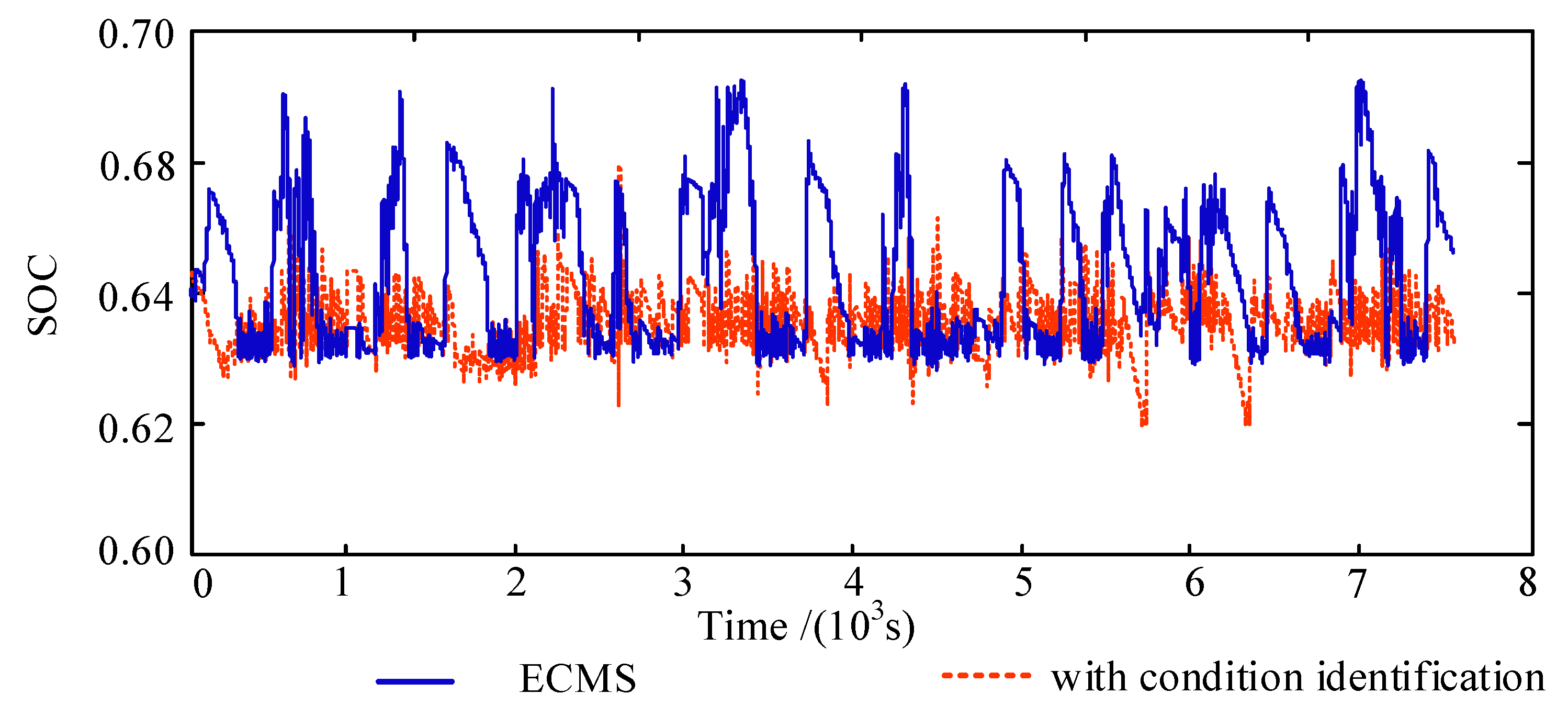
It is shown in Figure 15 and Figure 16 that with driving condition identification, the demanded torque is more appropriately distributed. Specifically, in congestion and urban conditions, the demanded torque is largely provided by the ISG alone, and the vehicle is more in purely electric operating mode. The rapid response of ISG is ideal for frequent start-and-stop, low speed and load, which reduces fuel consumption and emissions [13]. In suburban and highway conditions, the torque distribution between the ISG and the engine is better coordinated so that the engine operating points are kept closer to the optimal efficiency curve. Also, the ISG and engine torques are more consistent, which provides the HEV with smoother operation. Figure 14 demonstrates that under the selected random driving condition, the fuel consumption of the ECMS is 3.07 L, while the fuel consumption of the provided energy management strategy is 2.86 L, with a fuel consumption drop of 6.84%. In this study, the highest battery efficiency occurs when the SOC value is between 0.62 and 0.68. It can be seen from Figure 17 that when using the proposed energy management strategy, the SOC changes more smoothly, and is better maintained in the high-efficiency area. The results in the above figures indicate that the proposed energy management strategy based on driving condition identification using KGA-means is able to adjust the HEV power distribution between power sources, according to the change of driving conditions, which provides more efficient engine operation and maintains a SOC in a higher efficiency zone. As a result, the overall fuel consumption of the HEV is enhanced.
6. Conclusions
This study aims to achieve a practical energy management strategy based on driving condition identification, which can be readily applied to real vehicle controllers. The characteristic parameters of driving conditions are optimized, and then, an effective energy management strategy combined with a driving condition identification algorithm based on KGA-means and ECMS is proposed. The main contributions of this study are as follows:
- The experimental data is divided into driving condition segments, and the characteristic parameters of these driving condition segments are extracted. The correlation between characteristic parameters, the correlation between fuel consumption and characteristic parameters, and the sensitivity of characteristic parameters to driving conditions are carefully investigated. On this basis, the characteristic parameters of driving conditions are optimized, and vmean and rdrive are selected as the representative characteristic parameters.
- The K-means clustering algorithm is employed to identify driving conditions, and this identification method is combined with the ECMS to form a novel energy management strategy for HEVs.
- An HEV simulation model is established using MATLAB/Simulink. The simulation results show that using the proposed energy management strategy, the engine operating points are kept closer to the best efficiency curve, while the battery SOC changes more smoothly, and is maintained in a higher efficiency zone. As a result, the overall fuel consumption is reduced by 6.84%.
Author Contributions
Conceptualization, S.L.; Data curation, S.Z.; Formal analysis, S.Z.; Funding acquisition, M.H.; Investigation, S.L.; Methodology, S.L.; Project administration, M.H.; Resources, M.H.; Software, S.Z.; Supervision, D.Q.; Validation, C.G. and D.Q.; Visualization, C.G.; Writing-original draft, S.L.; Writing-review & editing, M.H., C.G. and D.Q.
Funding
This research was funded by the National Natural Science Foundation of the People’s Republic of China [No. 51675062], the National Key Research and Development Project [No. 2018YFB0106100], the Fundamental Research Funds for the Central Universities [No. 106112016CDJXZ338825], and the Major Program of Chongqing Municipality [No. cstc2015zdcy-ztzx60006].
Conflicts of Interest
The authors declare no conflict of interest.
References
- Sun, C.; He, H.; Sun, F. The Role of Velocity Forecasting in Adaptive-ECMS for Hybrid Electric Vehicles. Energy Procedia 2015, 75, 1907–1912. [Google Scholar] [CrossRef]
- Wang, J.; Wang, Q.N.; Zeng, X.H.; Wang, P.Y.; Wang, J.N. Driving cycle recognition neural network algorithm based on the sliding time window for hybrid electric vehicles. Int. J. Automot. Technol. 2015, 16, 685–695. [Google Scholar] [CrossRef]
- Zheng, C.; Xu, G.; Zhou, Y. Realization of PMP-based power management strategy for hybrid vehicles based on MPC scheme. In Proceedings of the IEEE International Conference on Information Science and Technology, Shenzhen, China, 26–28 April 2014; pp. 682–685. [Google Scholar]
- Guardiola, C.; Pla, B.; Reig, A. Modelling driving behavior and its impact on the energy management problem in hybrid electric vehicles. Int. J. Comput. Math. 2014, 91, 147–156. [Google Scholar] [CrossRef]
- Musardo, C.; Rizzoni, G.; Guezennec, Y.; Staccia, B. A-ECMS: An Adaptive Algorithm for Hybrid Electric Vehicle Energy Management. Decis. Control 2006, 11, 509–524. [Google Scholar]
- Datong, Q; Zhiyuan, P.; Yonggang, L.; Zhihui, D.; Yang, Y. Dynamic Energy Management Strategy of Hybrid Electric Vehicle Based on Driving condition Identification. China Mech. Eng. 2014, 25, 1550–1555. [Google Scholar]
- Guanlong, Y. Research on Energy Management Strategy of Plug-in Hybrid Vehicle Based on Driving Intention and Driving Condition Identification; Chongqing University: Chongqing, China, 2014. [Google Scholar]
- Zhuang, J.; Du, A.A. An Analysis on Quick Start of Engine in ISG HEV. Automot. Eng. 2008, 30, 305–308. [Google Scholar]
- Gurkaynak, Y.; Khaligh, A.; Emadi, A. Neural adaptive control strategy for hybrid electric vehicles with parallel powertrain. In Proceedings of the Vehicle Power and Propulsion Conference, Chicago, IL, USA, 6–9 September 2011. [Google Scholar]
- Huang, X.; Tan, Y.; He, X. An intelligent multi-feature statistical approach for discrimination of driving driving conditions of hybrid electric vehicle. In Proceedings of the International Joint Conference on Neural Networks, Atlanta, GA, USA, 14–19 June 2009. [Google Scholar]
- Guopeng, L. Control Strategy for Hybrid Buses Based on Road Driving Conditions and Load Status Identification; Tsinghua University: Beijing, China, 2011. [Google Scholar]
- Jeon, S.I.; Jo, S.T.; Lee, J.M. Multimode Driving Control of a Parallel Hybrid Electric Vehicle Using Driving Pattern Recognition. J. Dyn. Syst. Meas. Control. 2002, 124, 489–494. [Google Scholar] [CrossRef]
- Hongfei, H.; Xiangdong, H.; Yutao, L. HEV Real-time Equivalent Energy Consumption Minimum Control Strategy. Automot. Eng. 2006, 28, 516–520. [Google Scholar]
- Guohui, C.; Congbo, H. Research on the calculation method of automobile economy based on binary interpolation algorithm. Agric. Equip. Veh. Eng. 2012, 50, 26–28. [Google Scholar]
- Yiyou, L. Research on Power Balance Energy Management Control Strategy for Hybrid Hybrid Buses; Chongqing University: Chongqing, China, 2011. [Google Scholar]
Figure 1.
Structure of a hybrid electric vehicle (HEV) power system.

Figure 2.
Four typical driving conditions.

Figure 3.
Basic driving condition data.

Figure 4.
Schematic diagram of energy management strategy based on driving condition identification using a K-means clustering algorithm (KGA-means).
Figure 4.
Schematic diagram of energy management strategy based on driving condition identification using a K-means clustering algorithm (KGA-means).

Figure 5.
Two-dimensional scatter plot of driving condition segments.

Figure 6.
Result of the basic driving condition data clustering analysis.
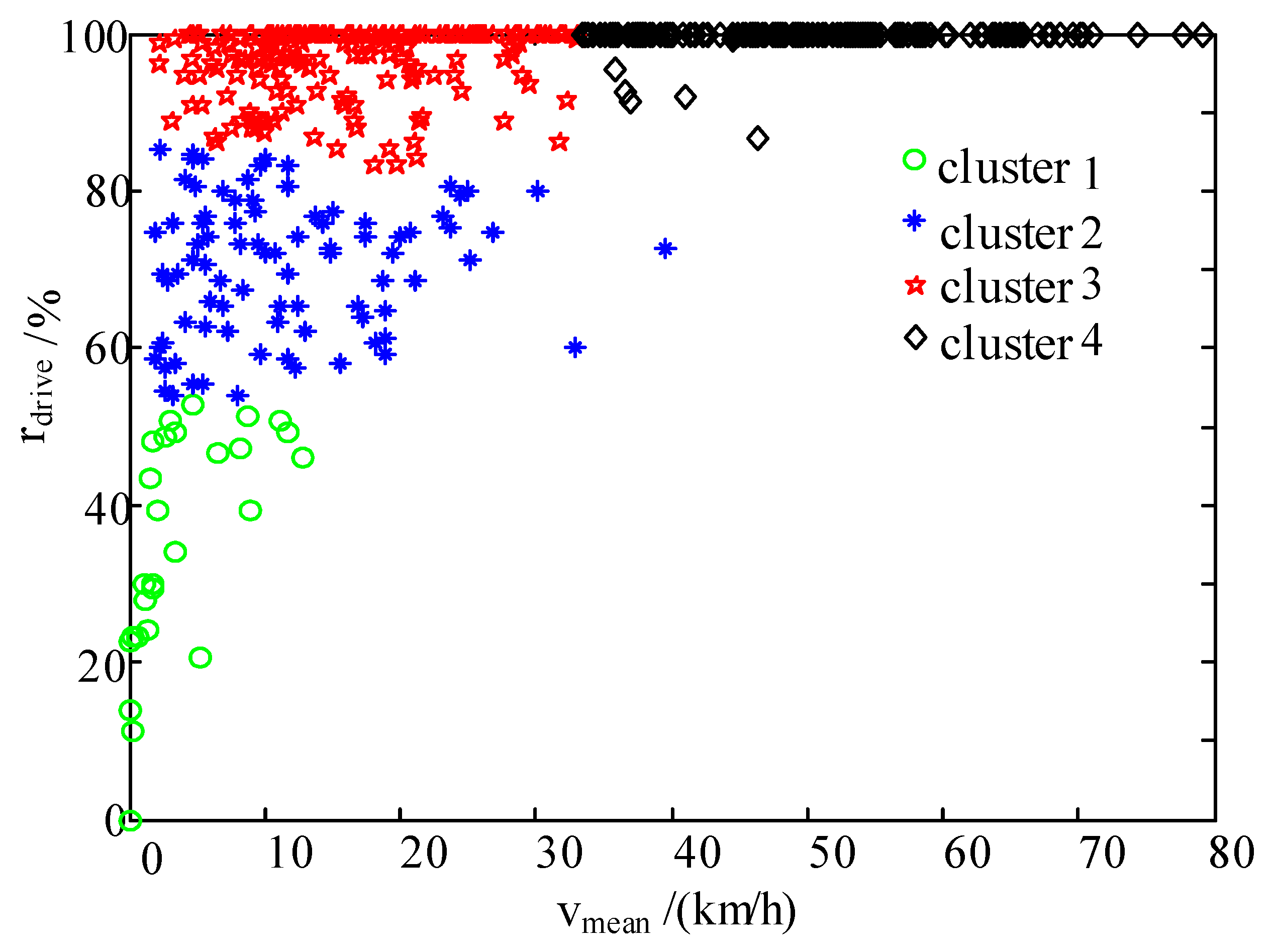
Figure 7.
Flow chart of the driving condition identification algorithm based on KGA-means.

Figure 8.
The relationship between the equivalent fuel consumption and the equivalent fuel coefficient under four typical cycle driving conditions.
Figure 8.
The relationship between the equivalent fuel consumption and the equivalent fuel coefficient under four typical cycle driving conditions.

Figure 9.
Optimal power distribution in urban condition with SOC values of 0.55 and 0.75.

Figure 10.
Optimal power distribution under the highway condition with SOC values of 0.55 and 0.75.

Figure 11.
HEV simulation model.

Figure 12.
Random driving condition.

Figure 13.
Identification results of the random driving condition.

Figure 14.
Fuel consumption of two different energy management strategies.

Figure 15.
Optimal torque distribution of two different energy management strategies.

Figure 16.
Engine-operating point of engine by two different energy management strategies.

Figure 17.
Battery SOC variations of two different energy management strategies.


Table 1.
Powertrain Parameters of HEV. CVT: continuously variable transmission; ISG: integrated starter and generator; SOC: state of charge.
Table 1.
Powertrain Parameters of HEV. CVT: continuously variable transmission; ISG: integrated starter and generator; SOC: state of charge.
| Parameter | Value | |
|---|---|---|
| Vehicle | Vehicle mass (kg) | 1547 |
| Windward area A (m2) | 2.28 | |
| Drag coefficient CD | 0.357 | |
| Wheel radius r (m) | 0.289 | |
| Rolling resistance coefficient fr | 0.0083 | |
| Engine | Maximum power (kW) | 85.1 |
| Maximum torque (Nm) | 160 | |
| ISG | Maximum power (kW) | 32 |
| Maximum torque (Nm) | 113 | |
| Battery | Capacity Q0 (Ah) | 40.5 |
| Nominal voltage U0(V) | 360 | |
| Initial SOC | 0.65 | |
| CVT | Speed ratio range iCVT | 0.422~2.432 |
| Main reduction ratio i0 | 5.297 | |
Table 2.
Correlation coefficients between the characteristic parameters.
| Rcor | vmean | vmax | amean | ridel | rdrive | … | s | vvar | vspa | aspa |
|---|---|---|---|---|---|---|---|---|---|---|
| vmean | 1.00 | 0.92 | 0.018 | −0.52 | 0.52 | … | 1 | 0.28 | 0.97 | 0.13 |
| vmax | 0.92 | 1.00 | −0.036 | −0.45 | 0.45 | … | 0.92 | 0.56 | 0.87 | 0.31 |
| amean | 0.018 | −0.036 | 1.00 | 0.0037 | −0.0037 | … | 0.011 | −0.17 | −0.049 | −0.060 |
| ameana | −0.026 | 0.14 | 0.18 | 0.098 | −0.098 | … | −0.026 | 0.26 | −0.065 | 0.84 |
| ameand | −0.12 | −0.28 | 0.16 | −0.035 | 0.035 | … | −0.12 | −0.39 | −0.069 | −0.87 |
| ridel | −0.52 | −0.45 | 0.037 | 1.00 | −1.00 | … | −0.52 | −0.063 | −0.41 | −0.010 |
| rdrive | 0.52 | 0.45 | −0.037 | −1.00 | 1.00 | … | 0.52 | −0.063 | −0.41 | −0.010 |
| amax | −0.18 | −0.056 | 0.073 | 0.22 | −0.22 | … | −0.18 | 0.19 | −0.19 | 0.70 |
| amin | −0.077 | −0.19 | 0.075 | −0.58 | 0.82 | … | −0.077 | −0.27 | −0.053 | −0.73 |
| s | 1 | 0.92 | 0.011 | −0.026 | −0.12 | … | 1.00 | 0.28 | 0.97 | 0.13 |
| vvar | 0.29 | 0.56 | −0.17 | −0.063 | 0.063 | 0.28 | 1.00 | 0.25 | 0.41 | |
| avar | 0.13 | 0.30 | −0.058 | −0.10 | 0.10 | … | 0.13 | 0.41 | 0.069 | 0.99 |
| vspa | 0.97 | 0.87 | −0.0049 | −0.41 | 0.41 | 0.97 | 0.25 | 1.00 | 0.071 | |
| aspa | 0.13 | 0.31 | −0.060 | −0.10 | 0.10 | … | 0.13 | 0.41 | 0.072 | 1.00 |
Table 3.
Correlation coefficients between fuel consumption and characteristic parameters.
| Rcor | vmean | vmax | amean | ameana | ameand | ridel | rdrive |
| Traditional vehicle fuel consumption | 0.915 | 0.838 | 0.162 | 0.109 | −0.170 | −0.386 | 0.386 |
| HEV fuel consumption | 0.957 | 0.894 | 0.144 | 0.145 | −0.238 | −0.475 | 0.475 |
| Rcor | amax | amin | s | vvar | avar | vspa | aspa |
| Traditional vehicle fuel consumption | −0.0691 | −0.1521 | 0.914 | 0.243 | 0.200 | 0.942 | 0.202 |
| HEV fuel consumption | −0.0484 | −0.200 | 0.957 | 0.287 | 0.267 | 0.956 | 0.270 |
Table 4.
Variation range and variation speed of characteristic parameters.
| Rcor | v mean | vmax | amean | ameana | ameand | ridel | rdrive |
| R1 | 0.334 | 0.318 | 0.688 | 0.116 | 0.210 | 0.269 | 0.269 |
| R2 | 0.859 | 0.772 | 0.956 | 0.260 | 0.478 | 0.551 | 0.551 |
| Rcor | amax | amin | s | vvar | avar | vspa | vspa |
| R1 | 0.112 | 0.193 | 0.334 | 0.214 | 0.180 | 0.293 | 0.180 |
| R2 | 0.288 | 0.491 | 0.859 | 0.363 | 0.362 | 0.680 | 0.364 |
Table 5.
Optimal equivalent fuel coefficients under four typical cycle driving conditions.
| Driving Condition | λchar Equivalent Fuel Coefficient When Charging | λdis Equivalent Fuel Coefficient When Discharging |
|---|---|---|
| Congestion condition | 1.1 | 3.0 |
| Urban condition | 5.0 | 2.8 |
| Suburban condition | 1.8 | 2.6 |
| Highway condition | 1.5 | 4.5 |
© 2018 by the authors. Licensee MDPI, Basel, Switzerland. This article is an open access article distributed under the terms and conditions of the Creative Commons Attribution (CC BY) license (http://creativecommons.org/licenses/by/4.0/).
Share and Cite
MDPI and ACS Style
Li, S.; Hu, M.; Gong, C.; Zhan, S.; Qin, D. Energy Management Strategy for Hybrid Electric Vehicle Based on Driving Condition Identification Using KGA-Means. Energies 2018, 11, 1531. https://doi.org/10.3390/en11061531
AMA Style
Li S, Hu M, Gong C, Zhan S, Qin D. Energy Management Strategy for Hybrid Electric Vehicle Based on Driving Condition Identification Using KGA-Means. Energies. 2018; 11(6):1531. https://doi.org/10.3390/en11061531
Chicago/Turabian StyleLi, Shuxian, Minghui Hu, Changchao Gong, Sen Zhan, and Datong Qin. 2018. "Energy Management Strategy for Hybrid Electric Vehicle Based on Driving Condition Identification Using KGA-Means" Energies 11, no. 6: 1531. https://doi.org/10.3390/en11061531
Note that from the first issue of 2016, this journal uses article numbers instead of page numbers. See further details here.