Impact of Plug-in Electric Vehicles Integrated into Power Distribution System Based on Voltage-Dependent Power Flow Analysis

Abstract

This paper proposes the impact of plug-in electric vehicles (PEVs) integrated into a power distribution system based on voltage-dependent control. The gasolinegate situation has many people turning to electric vehicles as a more environmentally friendly option, especially in smart community areas. The advantage of PEVs is modern vehicles that can use several types of fuel cells and batteries as energy sources. The proposed PEVs model was developed as a static load model in power distribution systems under balanced load conditions. The power flow analysis was determined by using certain parameters of the proposed electrical network. The main research objective was to determine the voltage magnitude profiles, the load voltage deviation, and total power losses of the electrical power system by using the new proposed methodology. Furthermore, it investigated the effects of the constant power load, the constant current load, the constant impedance load, and the plug-in electric vehicles load model. The IEEE 33 bus system was selected as the test system. The proposed methodology assigned the balanced load types in a steady state condition and used the new methodology to solve the power flow problem. The simulation results showed that increasing the plug-in electric vehicles load had an impact on the grids when compared with the other four load types. The lowest increased value for the plug-in electric vehicles load had an effect on the load voltage deviation (0.062), the total active power loss (120 kW) and the total reactive power loss (80 kVar), respectively. Therefore, this study verified that the load of PEVs can affect the electrical power system according to the time charging and charger position. Therefore, future work could examine the difference caused when PEVs are attached to the electrical power system by means of the conventional or complex load type.

1. Introduction

The transportation sector has become one of the main areas of energy consumption and has had a high impact on electrical power source sectors. Moreover, there have been several studies of new load characteristics that exist in electrical power systems. The plug-in electric vehicle (PEV) is a new electrical load type that is considered an emerging load in the focus area. The usage of PEVs has increased due to their low carbon emissions, promotion by governments, or privileges into certain special areas. The advantage of a PEV is that it utilizes both a fuel cell and battery as the energy source. The battery energy storage selected for use in PEVs can be converted and combined with the power to the traction motor drive systems. 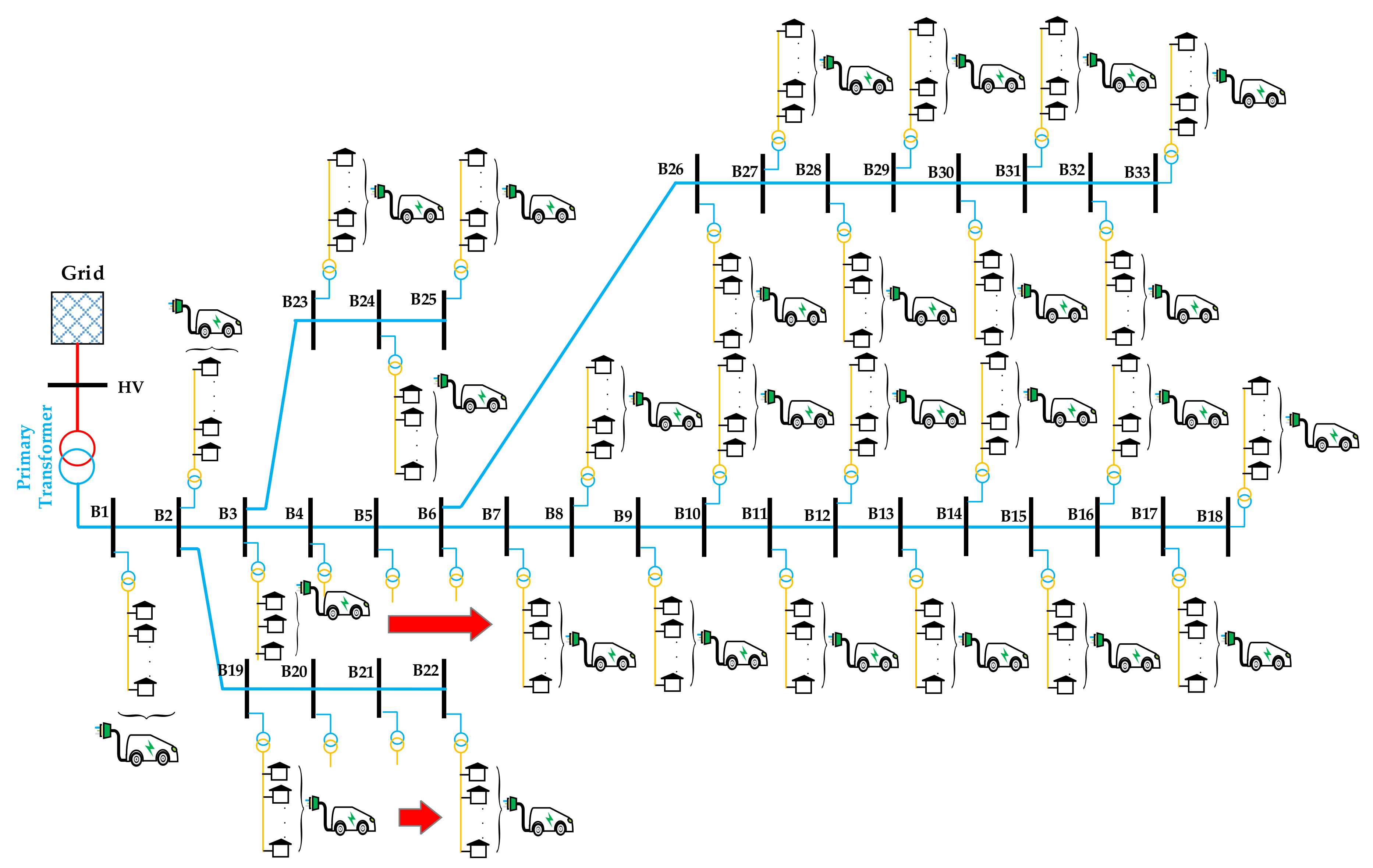The AC-DC converter has been used to convert electricity from the electrical power system to the battery as the charging state when the battery has a low level state-of-charge (SOC) [1]. Generally, the PEV charging condition is defined in normal charging mode for consuming electricity energy. The increasing penetration of PEVs will be connected to each household and consume energy as shown in Figure 1. Interestingly, the recharging condition of the PEV battery has been taking place on the grids simultaneously, so the power system will be impacted.

Meanwhile, the impact of electric vehicles on fast charging reduces the system voltage stability. Charging the battery depends on the charging type of the EVs battery installed at the charging stations [2]. Energy sources need to be supported under the power requirements of electrical equipment when the system is installed. Generally, the energy sources can be generated from conventional energy sources combined with renewable energy sources [3]. Therefore, a risk assessment was created for the electrical system using the charging behavior of electric vehicles. This can reduce the risk assessment on the power distribution system [4]. Both battery electric vehicles (BEVs) and plug-in hybrid electric vehicle loads (PHEVs) have been presented by considering the effect on vehicle-to-grid.(V2G) and grid-to-vehicle (G2V) power curves in terms of power demand [5]. The different level of penetration of BEVs and EVs will be directly impacted by the power demand response. The optimal management of charging should be considered under the demand response condition. The other uncertain propagation of charging from PEVs is affected by the aging of the power transformer. One type of methodology from smart charging is the coordinated charging of plug-in hybrid electric vehicles (PHEVs) that can reduce distribution system losses [6]. The literature [7] proposed an objective function from the triangle equivalence of losses, and load factor and load variance were used to find the optimal conditions on the PHEVs demand load profiles. Furthermore, the electrical power system networks were connected through a transmission lines system so that the distribution feeder reconfiguration could be adapted to manage the energy consumption from the PHEVs. This method can reduce the expected costs and total power loss reductions from the variance of penetration level of the PEVs in the electrical power system [8]. Additionally, the user’s benefits are becoming key issues to manage in terms of cost reduction which can be reduced battery capacity degradation, electricity cost, and the waiting time of charging queues at charging stations. Thus, the charging management should be controlled by optimal charging scheduling of EVs and provide maximum benefits for EV owners [9]. The aggregated EV charging demand needs to be determined and investigated in terms of any uncertain patterns of EV load in the electrical power system that are relevant to an agent-based approach. The agent-based approach consists of an EV type, battery and charging process, charging infrastructure, mobility, and society. Monte Carlo techniques were used to define the charging demand and charging scenarios, which revealed voltage profiles reduction during peak demand charging and should be controlled for the condition of balanced and unbalanced loads [10,11,12]. Consequently, the PEVs can reduce the impact from charging mode at the same time or in the same power transmission line by using V2G technology and in combination with smart grid control [1,13,14,15,16,17]. The smart grid control concept is needed to manage all the relevant areas in optimal condition such as power sources, transmission system, distribution system, user benefits, and economics [18,19,20]. Moreover, fast charging station in urban dwelling areas can be impacted by the electrical power system under conditions of voltage drop, transmission line loading, transformer loading, peak demand, and increase of total power loss [21,22]. Therefore, the electrical power system needs to be managed to reduce the factors that limit its capacity to provide sufficient energy. Interestingly, the electric vehicle integration in demand response (DR) programs can manage energy consumption at the customer side of the meter which can reduce peak demand and price volatility by utilizing smart grid enabling technologies. Moreover, the charging and discharging of EVs from the DR programs could be identified and evaluated in optimal conditions for the customer type in terms of DR programs and DR potential benefits [23]. Therefore, optimization techniques are applied to find the optimal solution to problems that affect the PEVs increase and high consumption of energy from the electrical power system networks [9,24,25,26]. Meanwhile, many current PEVs have been provided for users to replace the old internal combustion car, which are produced by different brands in the market. Furthermore, the Li-Ion battery is a popular and high-power density that is used in each PEV such as the Toyota Prius (PHEV2012), Chevrolet Volt, Mitsubishi i-MiEV, Nissan Leaf, and Tesla Roadster. Comparatively, the PHEVs and BEVs are a subset of the manufacture of PEVs with a higher distance efficiency as described in [27]. The authors in [28] executed V2G using bi-directional power flow and emergency power backup to reverse energy from the PEV’s battery to the apparatus of the house. However, the process of operating in V2G mode can increase battery wear and shorten the battery life. Therefore, the V2G setup needs to be managed in optimal condition and provide important services as well as balance renewable peak and bulk storage. The charging scheme and configuration of several PEVs are described in the International Electrotechnical Commission Standard (IEC 61851-1) and Society of Automotive Engineers standard (SAE J1772). Charging mode was defined in connection mode of DC power and AC power based on the battery charger and the position of charging such as normal charging mode used in residential distribution network. Therefore, the standard charging power levels of the IEC 61851-1 and SAE J1772 standard were used in private sectors, domestic environments, or public areas shown in

Table 1. Standard charging power levels in the IEC 61851-1 standard [29].

Connection Mode	Grid Connection	Voltage	Current	Type of Charge
Mode 1 (AC)	1 phase	230 V	16 A	Slow
	3 phase	400 V	16 A	Slow
Mode 2 (AC)	1 phase	230 V	32 A	Slow
	3 phase	400 V	32 A	Slow
Mode 3 (AC)	1 phase	230 V	32 A	Slow
	3 phase	690 V	250 A	Medium
Mode 4 (DC)	-	600 V	400 A	Fast

and

Table 2. Standard charging power levels in the SAE J1772 standard [17].

Type of Charge	Grid Connection	Voltage	Current	Type of Charge
AC level 1	1 phase	120 V	12–16 A	Slow
AC level 2	1 phase	240 V	<80 A	Slow
AC level 3	1, 3 phase	240 V	>80 A	Slow
DC level 1	-	200–450 V	80 A	Slow
DC level 2	-	200–450 V	200 A	Medium
DC level 3	-	200–600 V	400 A	Fast

as follows [17,29].

The PEV is a general term for any car that runs on battery energy storage and is recharged from the electricity grid in house hold. The PEV consists of battery electric vehicle (BEV) and plug-in hybrid vehicle (PHEV). The distance of PEVs driving has been defined based on battery sizing in kilowatt-hours (kWh) and rang of the electric (miles). For example, a PEV may be defined as a 53-mile Chevrolet Volt plug-in hybrid electric vehicle (PHEV) with 18.4 kWh battery. Meanwhile, a 335-mile BEV has been introduced, the Tesla model 3 100D with a 100 kWh battery, as shown in

Table 3. Comparison of the PEV types and technologies [30].

Manufacturer/Model	Type	Battery Size (kWh)	Electric Motor (kW)/Engine (L)	Range Electric (Miles)	Charging Rate (kW) [30,31]
Audi/A3 e-Tron	PHEV	8.8	75/1.4	16	3.3+
BMW/330e iPerformance	PHEV	7.6	65/2.0	22	1.4 */3.5+
BMW/i8 Coupe	PHEV	11.6	105.2/1.5	15	1.2 */3.7+
Chevrolet/Volt	PHEV	18.4	111/1.5	53	1.2 */3.6+
Ford/Fusion Energi SE	PHEV	7.6	88/2.0	21	*/3.3+
Honda/Clarity Plug-In Hybrid	PHEV	17	135.2/1.5	48	*/3.3+
Hyundai/Sonata	PHEV	9.8	50/2.0	27	*/3.3+
Mercedes/C350e	PHEV	6.2	60/2.0	20	3.3+
Toyota/Prius Prime	PHEV	8.8	60/1.8	25	*/3.3+
Porsche/Panamera S E-Hybrid	PHEV	14	101.45/4.0	16	3.3+
Volvo/XC90 T8	PHEV	10.4	65/2.0	19	3.3+
BMW/i3, i3s	BEV	33	126.82/135	114/107	1.2 */7.4+/DC
Chevrolet/Bolt	BEV	60	150	238	7.2+/DC
Fiat/500e	BEV	24	83	84	6.6+/DC
Honda/Clarity Electric	BEV	25.5	120	89	6.6+/DC
Hyundai/Ioniq Electric	BEV	28	88	124	6.6+/DC+
Nissan/Leaf	BEV	40	110	151	6.6+/DC
Smart ED	BEV	17.6	55	68	7.2+
Tesla/Model 3 Standard, Long Range	BEV	50,70	192.46, 202	220,310	*/+/DC+
Tesla/Model S 75D,100D and P100D	BEV	75,100,100	N/A	259,335,315	*/+/DC+
Tesla/Model X, 75D, 100D and P100D	BEV	75,100,100	N/A	237,295,289	*/11.5–17.2+/DC+
Kia/Soul EV	BEV	30	81.4	111	*/+/DC

Remark: * = AC level 1, + = AC level 2, DC = DC level 2, DC+ = DC level 3.

[30].

Table 3 shows the comparison of some PEV types and technologies from manufacturers around the world. There are defined based on the type of PEVs, battery size, electric motor/engine, range of electric driving, and charging rate of charger. Moreover, the battery capacity of PEVs related to PEVs driving distance that used energy source from the battery. The biggest motor sizing of BEV is the Tesla which is 3 long range model (202 kW), while the PHEV is Honda with Clarity Plug-In Hybrid model (135.2 kW). The sizing comparison of battery capacity was found that the maximum capacity of BEV is Tesla (model S, option 100D and P100D, or model X, option 100D and P100D rated 100 kWh) and the maximum capacity of PHEV is Chevrolet (model Volt rated 18.4 kWh).

The general practice of power flow study is to present the composite load characteristics at the point of common coupling of an electrical power system network. Meanwhile, the electrical load models consist of the static load model and dynamic load model. Therefore, the static load model is selected in static analysis for solving the power flow analysis using the conventional load $\left(Z,I,P\right)$ to represent each load model in the electrical power system [32]. The static load model consists of voltage dependency and frequency dependency of the load characteristics [33]. The battery charger in normal mode charging is represented by the characteristics of the PEVs, which is described in an exponential load by laboratory testing [34]. Many researchers have studied and found the impact of the PEVs on the electrical power system network as discussed in previous paragraphs, but they did not clarify and consider the actual behavior of the PEVs under voltage-dependent power flow analysis. For this reason, this article is going to investigate the PEVs load model based on the exponential load characteristics by considering the static load base. The PEV was defined in the behavior of general charging in normal charging rate that used the average value of charging rate remain about 1.2–3.7 kW of the PEV charger from Table 3. It means that the charging process took long time to charge the battery. Therefore, the charging levels of battery were defined on Mode 1 (IEC61851-1) or AC level 1 to 2 (SAE J1772) at standard outlet. However, PEV can generally be battery charge in Mode 1. There are consuming low power at 120–240 V range of the household and public area. So that, the load types were defined as a balanced load system that used for solving the impact from conventional load and PEVs to the electrical power system.

The structure of the paper is as follows: the load flow study (LF) for power flow analysis is presented in Section 2, as well as the proposed conventional load $\left(Z,I,P\right)$; PEVs based on static load models are presented in Section 3. Section 4 presents the total power losses in the electrical power system. The test radial distribution system is provided in Section 5. Section 6 proposes the simulation results and explanation. Finally, the conclusions and discussion are given in Section 7.

2. Proposed Load Flow Study and Formulation

The load flow study (LF) is very important in the planning of modern electrical power systems. In order to improve the existing system and it is pertinent to consider some of the issues that may affect the planning design, operation and control parts. The key point of LF the power system network is to use it to solve the steady state solution, which provides the information on voltage magnitude and phase angle, active and reactive power flow and total power loss. To understand the impacts of PEVs on the low voltage network (LV), it was defined as the amount of PEVs and behavioral uncertainties in a static power flow analysis framework from the proposed approach. The static power flow analysis was applied based on the voltage-dependent power flow that used to solve the impact form the load types. The PEVs were defined under the normal charging mode of the battery charger. The solving methodology is relevant based on three delivered metrics: the bus injection to branch injection matrix $\left[BIBC\right]$, the branch current to bus voltage matrix $\left[BCBV\right]$, and the current injection matrix $\left[I\right]$. This section applied the PEV’s load and analyzed the impact on the electrical power system as follows.

The $\left[BIBC\right]$, $\left[BCBV\right]$, and $\left[I\right]$ were simplified to analyze the radial distribution network (RDN) and could be adapted to the PEVs load into the algorithm [35]. Basically, the component of complex power load $\left(S_k\right)$ and injection current $\left(I_k^t\right)$ on the bus $k$ can be shown in Equations (1) and (2), respectively.

$$S_k=P_k+j{Q}_k\hspace{1em}\hspace{1em}\hspace{1em}k=1\dots N$$

(1)

where $N$ is the total number of buses in the radial distribution network. $P_k$ and $Q_k$ are the active power and reactive power of load at bus $k$.

Therefore, the equivalent injection current can be rearranged at the $t$ iteration of the solution from any bus to the $\left[I\right]$, as follows:

$$I_k^t=I_k^r\left(V_k^t\right)+j{I}_k^i\left(V_k^t\right)={\left(\frac{P_k+J{Q}_k}{V_k^t}\right)}^{\ast }$$

(2)

where $V_k^t$ is bus voltage and $I_k^t$ is equivalent injection current, respectively. Meanwhile, the equivalent injection current consists of a real part $\left(I_k^r\right)$ and an imaginary part $\left(I_k^i\right)$. Both the bus voltage and equivalent injection current are considered at the $t$ iteration of the solution.

Kirchhoff’s Current Law (KCL) was applied to solve the power flow of RDN from the relationship between the bus current injections and branch currents by formulating the branch currents from the current of any branch to the equivalent current injections as shown by

$$\left[B\right]=\left[BIBC\right]\left[I\right]$$

(3)

where $I$ represents the current injection matrix, $BIBC$ represents the branch injection to branch current matrix, and $B$ represents the current each branch. Generally, the $BIBC$ obtained number 1 or 0 only and upper triangular matrix.

Meanwhile, the relationship between the branch currents to the bus voltages can show a function of branch current, line parameters and the substation voltages as

$$\left[\Delta V\right]=\left[BCBV\right]\left[B\right]$$

(4)

where $BCBV$ represents the branch currents to bus voltages matrix and $\Delta V$ represents the voltage difference from the root node to each branch current.

The $BCVB$ and $BIBC$ were combined with the relation between the current injections and bus voltages of the RDN and can be expressed as

$$\begin{array}{c}\left[\Delta V\right]=\left[BCBV\right]\left[BIBC\right]\left[I\right]\\ =\left[DLF\right]\left[I\right]\end{array}\}$$

(5)

So, the voltage solution of the RDN each $t$ iteration can be expressed as

$$\left[\Delta V^{t+1}\right]=\left[DLF\right]\left[I^t\right]$$

(6)

3. Static Load Models and Load Voltage Deviation

3.1. Static Load Model

A load model of the electrical power system is defined by expressing the character instantaneous of time and then representing it as an algebraic function based on the frequency or the bus voltage magnitude at that instant. Basically, the apparent load power (kVA) can be separately considered from the active power component and the reactive power component, respectively. Generally, the voltage—dependent load behavior at each bus is represented by the exponential model in [33].

$$P_{Lk}=P_{Lk0}{\left(\frac{V_k}{V_{ko}}\right)}^{n_{pi}}$$

(7)

$$Q_{Lk}=Q_{Lk0}{\left(\frac{V_k}{V_{ko}}\right)}^{n_{qi}}$$

(8)

$$S_{Lk}=P_{Lk}+j{Q}_{Lk}$$

(9)

where $n$ indicates the amount of the PQ bus in the electrical power system; $S_{Lk}$, $P_{Lk}$, and $Q_{Lk}$ indicate the nominal apparent power, active power, and reactive power, respectively. Thus, $V_{i0}$ represents the magnitude of the bus nominal voltage. Meanwhile, $n_{pi}$ and $n_{qi}$ represent the load indices from each load type.

The PEV is a hybrid automobile combined with a combustion engine and an electric motor for the traction drive. Meanwhile, the energy source to feed the electric motor control with the battery can be recharged by connecting it to the electrical network. Therefore, the PEVs in the electrical network were represented by using the battery charger, which also converts the AC-DC converter for charging the battery. In order to define it in normal charging mode, the charger can be represented by the character instant of time as an algebraic function by using the exponential model, as in [34]. So, Equations (10) and (11) are concerned the load power factor value of the battery charger and will be considered when connected into the grid.

$$P_{PEVs}=S_0\times kp\times {\left(\frac{V_i}{V_{io}}\right)}^{n_{pi}}$$

(10)

$$Q_{PEVs}=S_0\times kq\times {\left(\frac{V_i}{V_{io}}\right)}^{n_{qi}}$$

(11)

$$S_{PEVs}=P_{PEV}+j{Q}_{PEV}$$

(12)

where $S_0$ indicates the apparent load power (kVA) at nominal voltage $V_{i0}$, $kp$ is representing the load power factor $\left(pf\right)$ and can be found by using $k_q=\sqrt{\left(1-p{f}^2\right)}$.

Table 4. Exponential indices value of load type.

Load Type	${\mathit{n}}_{\mathit{p}\mathit{i}}$	${\mathit{n}}_{\mathit{q}\mathit{i}}$
Constant impedance $\left(Z\right)$	2	2
Constant current $\left(I\right)$	1	1
Constant power $\left(P\right)$	0	0
PEVs [34]	2.59	4.06

shows the constant indices of load type used to solve the power flow problem on the electrical power system. The indices consisted of a constant impedance load, constant current load, constant impedance load and PEVs. The PEVs were specified on the normal charging model of the battery charger used in this study.

3.2. Load Voltage Deviation (LVD)

Accordingly, the increasing load on the power system will affect the voltage level in each bus. Therefore, the LVD was used to analyze the deviation of the bus voltage that was affected by the load. In general, the LVD value must be minimal, which shows that the system still has a good level of voltage. Therefore, the change in load on each bus must be appropriate, as described in Equation (13), [36,37].

$$LVD={{\displaystyle \sum _k^n\left(\frac{V_k^{ref}-V_k}{V_k^{ref}}\right)}}^2$$

(13)

where $V_k$ represents the bus load voltage of each load. Meanwhile, $V_k^{ref}$ represents the voltage reference under normal conditions that are also defined at 1 p.u.

4. Total Power Loss of Electrical Power System

Generally, all electrical appliances or loads of the electrical power system will be variable from the behavior of the load characteristics. Therefore, the total active and reactive power loss in the system used to evaluate the level of impact when the load increases in the electrical power system can be calculated from Figure 2 by using Equations (22) and (23) [38].

$$P_{k+1}=P_k-P_{Loss,k}-P_{LK+1}$$

(14)

$$=P_k-\frac{R_k}{{\left|V_k\right|}^2}\left\{P_k^2+{\left(Q_k+Y_k{\left|V_k\right|}^2\right)}^2\right\}-P_{Lk+1}$$

(15)

$$Q_{k+1}=Q_k-Q_{Loss,k}-Q_{Lk+1}$$

(16)

$$=Q_k-\frac{X_k}{{\left|V_k\right|}^2}\left\{P_k^2+{\left(Q_k+Y_{k1}{\left|V_k\right|}^2\right)}^2\right\}-Y_{k1}{\left|V_k\right|}^2-Y_{k2}{\left|V_{k+1}\right|}^2-Q_{Lk+1}$$

(17)

$${\left|V_{k+1}\right|}^2={\left|V_k\right|}^2+\frac{R_k^2+X_k^2}{{\left|V_k\right|}^2}\left(P_k^2+Q_k^2\right)-2\left(R_k{P}_k+X_k{Q}_k\right)$$

(18)

$$={\left|V_k\right|}^2+\frac{R_k^2+X_k^2}{{\left|V_k\right|}^2}\left(P_k^2+{\left(Q_k+Y_k{\left|V_k\right|}^2\right)}^2\right)-2\left(R_k{P}_k+X_k\left(Q_k+Y_k{\left|V_k\right|}^2\right)\right)$$

(19)

The active and reactive power in the transmission line section are connecting buses $k$ and $k+1$ which can be calculated as Equations (20) and (21), respectively.

$$P_{Loss}\left(k,k+1\right)=R_k\times \frac{\left(P_k^2+Q_k^2\right)}{{\left|V_k\right|}^2}$$

(20)

$$Q_{Loss}\left(k,k+1\right)=X_k\times \frac{\left(P_k^2+Q_k^2\right)}{{\left|V_k\right|}^2}$$

(21)

The power loss from a transmission line consists of active and reactive. Therefore, the total active power loss $\left(P_{T,loss}\right)$ and the total reactive power loss $\left(Q_{T,loss}\right)$ of the electrical power system are summarized as the losses of all transmission line in the system, which are given as Equations (22) and (23).

$$P_{T,Loss}={\displaystyle \sum _{k=1}^n{P}_{Loss}}\left(k,k+1\right)$$

(22)

$$Q_{T,Loss}={\displaystyle \sum _{k=1}^n{Q}_{Loss}}\left(k,k+1\right)$$

(23)

Using this efficient voltage-dependent power flow technique, the total losses and voltage at each bus of the electrical power system were assessed.

5. Proposed Radial Distribution System (RDS)

This study selected a primary distribution system to evaluate the impact of each load type on the power system network. The IEEE 33 bus test system has been used to obtain results and to evaluate the efficiency of each type of load test by determining the base megavolt-ampere (MVA) = 100 MVA, base voltage = 11 kV. The selected IEEE 33 bus test system was define d as consisting of 32 line sections with a total power constant load of 3.72 MW and 2.3 MVar in the balanced load system, as shown in [39]. Therefore, this article considered solving the impact of PEVs integrated into power distribution system, based on a voltage-dependent power flow analysis. The test system was modified from the traditional load models to voltage-dependent load models. The LF methodology was applied to analyze and compare each load type by using voltage profiles, total power loss, and LVD under balanced load condition for any load type installation as shown in Table 4.

6. Simulation Results

The proposed load types and LF algorithm were implemented in a MATLAB m-file and the algorithm is shown in the Appendix A. The static analysis of LF was solved based on the balanced load of a constant impedance load $\left(Z\right)$, constant current load $\left(I\right)$, constant power load $\left(P\right)$, and PEVs. This article supposed that each load type installed in the electrical system was the same load for each iteration and the load type change was well done. Therefore, the number of conventional loads $\left(Z,I,P\right)$ and PEVs will each be distributed at the RDS bus. The simulation results show the bus voltage, total power loss, and LVD for each type of load as given in

Table 5. Comparison voltage profiles of IEEE 33 bus test system load-flow results.

Bus No.	$\mathit{Z}$ (p.u.)	$\mathit{I}$ (p.u.)	$\mathit{P}$ (p.u.)	PEVs (p.u.)
1	1.0000	1.0000	1.0000	1.0000
2	0.9973	0.9972	0.9970	0.9977
3	0.9847	0.9839	0.9829	0.9873
4	0.9782	0.9769	0.9755	0.9820
5	0.9717	0.9701	0.9681	0.9768
6	0.9558	0.9530	0.9497	0.9631
7	0.9527	0.9498	0.9462	0.9602
8	0.9485	0.9453	0.9413	0.9572
9	0.9432	0.9395	0.9351	0.9532
10	0.9382	0.9342	0.9292	0.9494
11	0.9374	0.9334	0.9284	0.9489
12	0.9362	0.9320	0.9269	0.9480
13	0.9310	0.9264	0.9208	0.9441
14	0.9290	0.9243	0.9185	0.9426
15	0.9278	0.9230	0.9171	0.9418
16	0.9267	0.9218	0.9157	0.9410
17	0.9250	0.9199	0.9137	0.9396
18	0.9245	0.9194	0.9131	0.9392
19	0.9968	0.9967	0.9965	0.9972
20	0.9933	0.9931	0.9929	0.9939
21	0.9926	0.9924	0.9922	0.9932
22	0.9919	0.9918	0.9916	0.9926
23	0.9813	0.9804	0.9794	0.9843
24	0.9750	0.9739	0.9727	0.9788
25	0.9719	0.9707	0.9694	0.9760
26	0.9541	0.9512	0.9477	0.9617
27	0.9519	0.9489	0.9452	0.9598
28	0.9421	0.9383	0.9337	0.9507
29	0.9350	0.9308	0.9255	0.9441
30	0.9320	0.9275	0.9220	0.9414
31	0.9285	0.9237	0.9178	0.9385
32	0.9277	0.9229	0.9169	0.9378
33	0.9274	0.9226	0.9166	0.9376

, Figure 3;

Table 6. Comparison of the 33 bus test system from the lines active power loss results.

Br. No.	$\mathit{Z}$ (kW)	$\mathit{I}$ (kW)	$\mathit{P}$ (kW)	PEVs (kW)
1	10.031	10.999	12.240	7.613
2	41.469	45.975	51.791	30.940
3	15.190	17.217	19.900	11.499
4	14.134	16.095	18.699	10.615
5	28.793	32.849	38.249	21.652
6	1.457	1.654	1.915	0.868
7	3.625	4.145	4.838	2.094
8	3.075	3.546	4.181	1.693
9	2.606	3.012	3.561	1.471
10	0.404	0.467	0.554	0.235
11	0.640	0.742	0.881	0.359
12	1.927	2.240	2.666	1.033
13	0.526	0.612	0.729	0.265
14	0.256	0.299	0.357	0.094
15	0.201	0.235	0.281	0.091
16	0.179	0.210	0.252	0.086
17	0.038	0.044	0.053	0.021
18	0.157	0.159	0.161	0.140
19	0.807	0.819	0.832	0.707
20	0.098	0.099	0.101	0.085
21	0.042	0.043	0.044	0.037
22	2.852	3.005	3.182	2.144
23	4.596	4.850	5.144	3.402
24	1.143	1.210	1.287	0.835
25	1.931	2.217	2.601	1.789
26	2.460	2.831	3.329	2.328
27	8.315	9.588	11.301	8.052
28	5.751	6.638	7.833	5.746
29	2.853	3.297	3.896	2.955
30	1.154	1.341	1.594	0.711
31	0.154	0.179	0.213	0.098
32	0.010	0.011	0.013	0.008

and

Table 7. Comparison of load voltage deviation (LVD), total active power loss and total reactive power loss.

Load Type	LVD	Active Power Loss (kW)	Reactive Power Loss (kVar)	Apparent Power Loss (kVA)	%LVD	%P loss	%Q loss
PEVs	0.062	119.67	79.31	143.56	−40.96%	−41.31%	−41.07%
$Z$	0.089	156.87	104.18	188.31	−22.60%	−22.91%	−22.70%
$I$	0.101	176.63	117.51	212.15	−12.85%	−13.04%	−12.91%
$P$ [38,40]	0.117	202.68	135.14	243.60	0.00%	0.00%	0.00%

and Figure 4, respectively.

It is possible to see the voltage magnitude profiles arranged from bus No. 1 to bus No. 33 under different load types and voltage levels as shown in Table 5. Therefore, the effect of load and transmission line decreased the level of the voltage profile and increased the total power loss. The results of the voltage magnitude profiles were derived from the voltage-dependent power flow analysis of different load types. The simulation results showed the lowest voltage of each load type on bus No. 18 (the bold text number). The comparison on bus No. 18 from the highest to the lowest of the voltage magnitudes were PEVs load (0.9392 p.u.), $Z$ load (0.9392 p.u.), $I$ load (0.9392 p.u.), and $P$ load (0.9392 p.u.), respectively. Therefore, the static voltage magnitude profiles of each load type found the weak point of the lowest voltage magnitude profile from the $P$ load when compared to the $Z$ load, $I$ load and PEVs load.

Figure 3 shows the contour of the static voltage magnitude profiles compared with the $Z$ load, $I$ load, $P$ load, and PEVs, respectively. The graphics showed that the lowest contour voltage profiles remained at about 0.9130 p.u. (red color field) and the highest contour voltages profiles remained at about 1 p.u. (violets color field). The static voltage analysis, by applying contour color, can show some details of the characteristics of any load type. Exclusively, the PEVs’ load contour of static voltage magnitude profiles were shown, which affected the lowest level when compared with any load type. Therefore, the $Z$ load, $I$ load, $P$ load, and PEVs affect are considered to be static voltage stability based on the voltage profiles obtained from the electrical power system. In decreasing order, the factors that affected the static voltage stability were the $P$ load, $I$ load, $Z$ load, and PEVs.

Table 6 demonstrates all of the effects from each load model type to the transmission line losses from transmission line No. 1 to transmission line No. 32. The total power losses were derived from the current flow throughout a transmission line between two buses that affect the load were installed on any of the buses. The sizing and location of the transmission line loss resulted in a voltage drop in the power system and in condition to install near the root node that should carry the burden from the current to the end of the node. However, many factors and details affect the loss from the cable such as temperature, installation method, type of cable, and so on. The simulation results are going to show the power losses in kilowatt (kW) of RDN transmission lines. In this case, transmission line No. 2 was affected more than the transmission line loading of each transmission line. The comparison on transmission line No. 2 from the highest to the lowest of the lines’ active power loss (the bold text number) were $P$ load (51.791 kW), $I$ load (45.975 kW), $Z$ load (41.469 kW) and PEVs load (30.940 kW). Accordingly, if compared on the second order from the highest to the lowest of the lines active power loss (the underline text number) were found on transmission line number No. 5, it was $P$ load (38.249 kW), $I$ load (32.849 kW), $Z$ load (28.793 kW), and PEVs (21.652 kW). Comparatively, the total power loss in the transmission lines can be reduced to improve its voltage stability.

The results from Figure 4 were compared with the contour of lines of the active power loss magnitude profiles obtained for each load type in the test system. All simulation results showed the effect of the active power loss profiles for each load type on the different lines. Figure 4 shows that the highest active power loss of load types of the red color contour was at transmission line number No. 2, and the second order of highest active power loss of the load types on the yellow color contour in transmission line of number No.5. The simulation results from the contour with different load types showed the weak point of the highest active power loss on the transmission lines.

From the results above, it can be observed that all voltage profiles and all transmission line losses were effected from the conventional load type and PEVs. The exponential indices of load types were applied to analyze the impact of the grid. Therefore, the optimal model of load type could be selected and nearly defined the behavior of each load type.

Table 7 shows that the results of the LF algorithm based on the voltage-dependent power flow analysis. The simulation results were compared the values of the total real power loss, the total reactive power loss and LVD. The total active power loss and the total reactive power loss of the PEVs were shown to be less than those of the $Z$, $I$ and $P$ load. Additionally, the comparison of the LVD and the total power loss in percentages was defined as the base case from the $P$ load. The percentages of the PEVs showed the lowest when compared to the percentages of each load type. Therefore, the low level of the percentages indicated the low impact to the grid in terms of the LVD and the total power loss. Interestingly, the PEVs showed that it was not significant from the voltage magnitude profile and total power loss of the electrical power system. Generally, PEVs are connected with another load into the network. The system management should consider the impact at this point when there is a large-scale PEV penetration with the conventional load of the grid.

Thus, it is important to highlight that the effects on the LVD, total active power, and total reactive power are dependent on the type of the load model installed in the RDS. Furthermore, the PEV model was affected less than the $Z$, $I$ and $P$ load, in order to compare them one by one. Therefore, the PEVs affect to the electrical power system when plugged into the power system network with the traditional load. Moreover, the high penetration level of PEVs is connected to the grid need to be managed in the optimal condition.

7. Conclusions

This article analyzed the impact of PEVs based on a voltage-dependent power flow analysis. This study shows the static voltage stability on the proposed PEVs integrated into the electrical power system using the new LF methodology. The MATLAB program environment was selected to solve the new proposed algorithm using m-files script base. The proposed LF methodology was tested in the IEEE 33 bus system. The simulation results showed that the LVD and total power losses were shown the performance of PEVs load compared with the three conventional loads. The exponential index of the load types will be the main influence to analytical effect on the voltage-dependent power flow analysis. The effect of PEVs load had the voltage stability effect to the power grids less than a constant power load, constant current load, and constant impedance load. The PEVs test case expressed the lowest LVD, and the lowest total power loss values were 0.062, 120 kW and 80 kVar. The comparisons of PEVs showed that the lowest from the percentage of LVD (−40.96%), active power loss (−41.31%) and reactive power loss (−41.07%), respectively. The results confirmed that the proposed PEVs model had a low impact on the grid when compared with the conventional load. However, the voltage-dependent power flow analysis could be considered as a different level of PEVs load. The light to level of PEVs load had no impact on the grid, but the large scale of PEVs load had a greater effect on the grid. Furthermore, the proper management of PEVs can be benefited to reduce the impact of the electrical power system in each area of the battery charger. It can also be implemented in other conditions with PEVs charging clustered by coordinating each charger. The conclusion can provide the design guidance for EV charging station and power system planning for PEVs in the future.

References

1. Yilmaz, M.; Krein, P.T. Review of the Impact of Vehicle-to-Grid Technologies on Distribution Systems and Utility Interfaces. IEEE Trans. Power Electron. 2013, 28, 5673–5689. [Google Scholar] [CrossRef]
2. Dharmakeerthi, C.H.; Mithulananthan, N.; Saha, T.K. Impact of electric vehicle fast charging on power system voltage stability. Int. J. Electr. Power Energy Syst. 2014, 57, 241–249. [Google Scholar] [CrossRef]
3. Hidayatullah, N.A.; Stojcevski, B.; Kalam, A. Analysis of Distributed Generation Systems, Smart Grid Technologies and Future Motivators Influencing Change in the Electricity Sector. Smart Grid Renew. Energy 2011, 2, 216. [Google Scholar] [CrossRef]
4. Yang, J.; Hao, W.; Chen, L.; Chen, J.; Jin, J.; Wang, F. Risk Assessment of Distribution Networks Considering the Charging-Discharging Behaviors of Electric Vehicles. Energies 2016, 9, 560–580. [Google Scholar] [CrossRef]
5. Aziz, M.; Oda, T.; Mitani, T.; Watanabe, Y.; Kashiwagi, T. Utilization of Electric Vehicles and Their Used Batteries for Peak-Load Shifting. Energies 2015, 8, 3720–3738. [Google Scholar] [CrossRef] [Green Version]
6. Cao, C.; Wang, L.; Chen, B. Mitigation of the Impact of High Plug-in Electric Vehicle Penetration on Residential Distribution Grid Using Smart Charging Strategies. Energies 2016, 9, 1024–1049. [Google Scholar] [CrossRef]
7. Sortomme, E.; Hindi, M.M.; MacPherson, S.D.J.; Venkata, S.S. Coordinated Charging of Plug-In Hybrid Electric Vehicles to Minimize Distribution System Losses. IEEE Trans. Smart Grid 2011, 2, 198–205. [Google Scholar] [CrossRef]
8. Rostami, M.A.; Kavousi-Fard, A.; Niknam, T. Expected Cost Minimization of Smart Grids With Plug-In Hybrid Electric Vehicles Using Optimal Distribution Feeder Reconfiguration. IEEE Trans. Ind. Inform. 2015, 11, 388–397. [Google Scholar] [CrossRef]
9. Su, S.; Li, H.; Gao, D. Optimal Planning of Charging for Plug-In Electric Vehicles Focusing on Users’ Benefits. Energies 2017, 10, 952–967. [Google Scholar] [CrossRef]
10. Olivella-Rosell, P.; Villafafila-Robles, R.; Sumper, A.; Bergas-Jané, J. Probabilistic Agent-Based Model of Electric Vehicle Charging Demand to Analyse the Impact on Distribution Networks. Energies 2015, 8, 4160–4187. [Google Scholar] [CrossRef] [Green Version]
11. Schimpe, M.; Piesch, C.; Hesse, H.; Paß, J.; Ritter, S.; Jossen, A. Power Flow Distribution Strategy for Improved Power Electronics Energy Efficiency in Battery Storage Systems: Development and Implementation in a Utility-Scale System. Energies 2018, 11, 533–550. [Google Scholar] [CrossRef]
12. Ul-Haq, A.; Azhar, M.; Mahmoud, Y.; Perwaiz, A.; Al-Ammar, E. Probabilistic Modeling of Electric Vehicle Charging Pattern Associated with Residential Load for Voltage Unbalance Assessment. Energies 2017, 10, 1351–1369. [Google Scholar] [CrossRef]
13. Ali, A.; Söffker, D. Towards Optimal Power Management of Hybrid Electric Vehicles in Real-Time: A Review on Methods, Challenges, and State-Of-The-Art Solutions. Energies 2018, 11, 476–490. [Google Scholar]
14. Rottondi, C.; Fontana, S.; Verticale, G. Enabling Privacy in Vehicle-to-Grid Interactions for Battery Recharging. Energies 2014, 7, 2780–2798. [Google Scholar] [CrossRef] [Green Version]
15. Erdinc, O.; Paterakis, N.G.; Mendes, T.D.P.; Bakirtzis, A.G.; Catalão, J.P.S. Smart Household Operation Considering Bi-Directional EV and ESS Utilization by Real-Time Pricing-Based DR. IEEE Trans. Smart Grid 2015, 6, 1281–1291. [Google Scholar] [CrossRef]
16. Kim, B.G.; Ren, S.; Schaar, M.V.D.; Lee, J.W. Bidirectional Energy Trading and Residential Load Scheduling with Electric Vehicles in the Smart Grid. IEEE J. Sel. Areas Commun. 2013, 31, 1219–1234. [Google Scholar] [CrossRef]
17. Yuttana, K.; Wannawit, J.; Krischonme, B.; Nadarajah, M. Estimation of the Quick Charging Station for Electric Vehicles based on Location and Population Density Da. Int. J. Intell. Eng. Syst. 2018, 11, 233–241. [Google Scholar]
18. Maigha, C.M. Economic Scheduling of Residential Plug-In (Hybrid) Electric Vehicle (PHEV) Charging. Energies 2014, 7, 1876–1898. [Google Scholar] [CrossRef] [Green Version]
19. Yoon, S.-G.; Kang, S.-G. Economic Microgrid Planning Algorithm with Electric Vehicle Charging Demands. Energies 2017, 10, 1487–1503. [Google Scholar] [CrossRef]
20. Ma, T.; Mohammed, O.A. Economic Analysis of Real-Time Large-Scale PEVs Network Power Flow Control Algorithm With the Consideration of V2G Services. IEEE Trans. Ind. Appl. 2014, 50, 4272–4280. [Google Scholar] [CrossRef]
21. Mauri, G.; Valsecchi, A. Fast charging stations for electric vehicle: The impact on the mv distribution grids of the milan metropolitan area. In Proceedings of the 2012 IEEE International Energy Conference and Exhibition (ENERGYCON), Florence, Italy, 9–12 September 2012; pp. 1055–1059. [Google Scholar]
22. Grackova, L.; Oleinikova, I. Impact of electric vehicle charging on the urban distribution network. In Proceedings of the 2016 57th International Scientific Conference on Power and Electrical Engineering of Riga Technical University (RTUCON), Riga&Cesis, Latvia, 13–14 October 2016; pp. 1–5. [Google Scholar]
23. Falvo, M.C.; Graditi, G.; Siano, P. Electric Vehicles integration in demand response programs. In Proceedings of the 2014 International Symposium on Power Electronics, Electrical Drives, Automation and Motion, Ischia, Italy, 18–20 June 2014; pp. 548–553. [Google Scholar]
24. Gao, B.; Zhang, W.; Tang, Y.; Hu, M.; Zhu, M.; Zhan, H. Game-Theoretic Energy Management for Residential Users with Dischargeable Plug-in Electric Vehicles. Energies 2014, 7, 7499–7518. [Google Scholar] [CrossRef] [Green Version]
25. Liu, H.; Ji, Y.; Zhuang, H.; Wu, H. Multi-Objective Dynamic Economic Dispatch of Microgrid Systems Including Vehicle-to-Grid. Energies 2015, 8, 4476. [Google Scholar] [CrossRef]
26. Khaled, U.; Eltamaly, A.M.; Beroual, A. Optimal Power Flow Using Particle Swarm Optimization of Renewable Hybrid Distributed Generation. Energies 2017, 10, 1013. [Google Scholar] [CrossRef]
27. Yilmaz, M.; Krein, P.T. Review of Battery Charger Topologies, Charging Power Levels, and Infrastructure for Plug-In Electric and Hybrid Vehicles. IEEE Trans. Power Electron. 2013, 28, 2151–2169. [Google Scholar] [CrossRef]
28. Meintz, A.; Markel, T.; Jun, M.; Zhang, J. Integrating PEVs with Renewables and the Grid; Office of the Assistant Secretary of Energy Efficiency and Renewable Energy: Washington, DC, USA, 2016. [Google Scholar]
29. Alonso, M.; Amaris, H.; Germain, J.; Galan, J. Optimal Charging Scheduling of Electric Vehicles in Smart Grids by Heuristic Algorithms. Energies 2014, 7, 2449. [Google Scholar] [CrossRef]
30. Compare Vehicles. Available online: https://pluginamerica.org/vehicles/ (accessed on 6 June 2018).
31. Compare Electric Cars and Plug-in Hybrids by Features, Price, Range. Available online: http://www.plugincars.com/cars (accessed on 6 June 2018).
32. Martí, J.R.; Ahmadi, H.; Bashualdo, L. Linear Power-Flow Formulation Based on a Voltage-Dependent Load Model. IEEE Trans. Power Deliv. 2013, 28, 1682–1690. [Google Scholar] [CrossRef]
33. Kundur, P. Power System Stability and Control; McGraw-Hill: New York, NY, USA, 1994; pp. 272–273. [Google Scholar]
34. Hajagos, L.M.; Danai, B. Laboratory measurements and models of modern loads and their effect on voltage stability studies. IEEE Trans. Power Syst. 1998, 13, 584–592. [Google Scholar] [CrossRef]
35. Jen-Hao, T. A direct approach for distribution system load flow solutions. IEEE Trans. Power Deliv. 2003, 18, 882–887. [Google Scholar] [CrossRef]
36. Kongjeen, Y.; Bhumkittipich, K. Modeling of electric vehicle loads for power flow analysis based on PSAT. In Proceedings of the 2016 13th International Conference on Electrical Engineering/Electronics, Computer, Telecommunications and Information Technology (ECTI-CON), Chiang Mai, Thailand, 28 June–1 July 2016; pp. 1–6. [Google Scholar]
37. Kongjeen, Y.; Buayai, K.; Bhumkittipich, K. Automate of capacitor placement in microgrid system under EVs load penetration. In Proceedings of the 2017 International Electrical Engineering Congress (iEECON), Pattaya, Thailand, 8–10 March 2017; pp. 1–4. [Google Scholar]
38. Rao, R.S.; Ravindra, K.; Satish, K.; Narasimham, S.V.L. Power Loss Minimization in Distribution System Using Network Reconfiguration in the Presence of Distributed Generation. IEEE Trans. Power Syst. 2013, 28, 317–325. [Google Scholar] [CrossRef]
39. Baran, M.E.; Wu, F.F. Network reconfiguration in distribution systems for loss reduction and load balancing. IEEE Trans. Power Deliv. 1989, 4, 1401–1407. [Google Scholar] [CrossRef]
40. Mishra, S.; Das, D.; Paul, S. A simple algorithm for distribution system load flow with distributed generation. In Proceedings of the International Conference on Recent Advances and Innovations in Engineering (ICRAIE-2014), Jaipur, India, 9–11 May 2014; pp. 1–5. [Google Scholar]
Figure 1. Plug-in electric vehicles (PEVs) connected in a radial distribution system.
Energies 11 01571 g001
Figure 2. Electrical equivalent circuit of a typical branch k
Energies 11 01571 g002
Figure 3. Contour of static voltage profiles from difference load type.
Energies 11 01571 g003
Figure 4. Contour of lines active power losses when difference load type.
Energies 11 01571 g004