Distributed Energy Sharing for PVT-HP Prosumers in Community Energy Internet: A Consensus Approach


1
State Key Laboratory of Alternate Electrical Power System with Renewable Energy Sources, North China Electric Power University, Beijing 102206, China
2
School of Economics and Management, North China Electric Power University, Beijing 102206, China
*
Author to whom correspondence should be addressed.
Energies 2018, 11(7), 1891; https://doi.org/10.3390/en11071891
Submission received: 27 June 2017
/
Revised: 15 July 2018
/
Accepted: 17 July 2018
/
Published: 20 July 2018
(This article belongs to the Special Issue Optimization Methods Applied to Power Systems)
Abstract
:Community Energy Internet (CEI) integrates electric network and thermal network based on combined heat and power (CHP) to improve the economy of energy system in Smart Community. In the CEI, an energy sharing framework for prosumers equipped with photovoltaic-thermal (PVT) system and heat pump (HP) is introduced. Supporting by the PVT and HP, the prosumer has four role attributes with either heat or electricity producer/consumer. A social welfare maximization model is built for the CEI, including PVT-HP prosumers, CHP system, and utility grid. Considering there are multiply participants in the local market of CEI, the social welfare maximization problem is decoupled by using Lagrange multiplier method. Moreover, a consensus-based fully distributed algorithm is designed to solve the problem. Finally, six residential buildings are selected as the case study to validate the effectiveness of the proposed method.
1. Introduction
Energy Internet (EI) was proposed [1] to improve the utilization of renewable energy and meet the growing demand for energy. EI is a highly intelligent system which integrates distributed energy resources (DERs) and advanced Internet technology with existing Smart Grid [2]. A variety of energy, especially the renewable energy including photovoltaic (PV), wind turbine (WT), can be absorbed in a dynamic means for the distributed topology of the power network [3]. Furthermore, the power loss reduction, energy utilization efficiency improvement, and energy demand allocation optimization can be achieved under the EI [4]. From the perspective of energy policy, in China, the government has developed a series of energy policies, i.e., changing fuel from coal to natural gas and renewable energy. As a core component of the EI, the combined heat and power (CHP), PV and heat pump are bound to realize the goal and enhance the energy transaction efficiency.
Until recently, the research of the EI has drawn wide attention, and its topics may include architecture system [5,6,7], coordination control [8,9] and energy management [10,11,12]. A future electric power distribution system was proposed in [5] to suit for the plug-and-play of DERs and distributed storage devices. The main features of the future electric power distribution system is discussed in [6]. Based on the EI, a three-phase cascaded power electronic transformer was designed to connect with high voltage directly [7]. Energy hub is an effective means to realize reliable control of the EI. A decentralized model predictive control strategy was proposed in [8] to improve the operation of the coupled electricity and gas network system by considering predicted behavior and operational constraints. A residential energy hub is designed to coordinate solar energy with load demand and determine the scheduling of electric vehicles [9]. Particularly, there are multiple participants inside an EI, how to coordinate and optimize the interests of each participant is addressed in [10,11,12,13]. An optimization model of energy sharing among smart building is developed using non-cooperative game theory [10]. To improve the economy and reliability, a distributed energy management is proposed for interconnected CHP-based Microgrids with demand response (DR) [11]. Based on the feed-in-tariff, an energy sharing model is formulated among peer-to-peer PV prosumers [12].
It is worth noting that the electric efficiency of a PV panel is less than 20% in practical operation while the rest 80% of solar radiation is wasted into other forms of energy [14]. Hence, solar photovoltaic-thermal (PVT) hybrid system is proposed to improve both the electrical efficiency and the thermal efficiency [15]. Furthermore, the study in [16] shows that the idea of PVT system is economically feasible. However, the hot water produced by PVT system cannot meet the application requirements of temperature, from [17,18,19], it is demonstrated that working with a heat pump, PVT system will significantly increase system efficiency and provides both electricity and thermal energy for end users. Fuzzy Logic control has been applied to optimize the energy consumption of the PVT system [17]. A thermodynamics model is built for a refrigerant-based PVT assisted heat pump water heater system in [18]. A practical residential application of heat pump coupled with a PVT system is addressed in [19], the system can provide space heating and domestic hot water for a single-family dwelling located in North East Italy. PV panels of PVT combined with heat pump system can produce more additional power compared with the uncooled one [20]. In this paper, the end user equipped with PVT system and heat pump is named as a PVT-HP prosumer.
Distributed energy management has been widely used in Smart Grid for privacy protection [21], high efficiency [22], and global fairness [23]. Among them, consensus algorithm is considered to be an important solution for Smart Grid in a multi-agent system. For the economic dispatch problem, the traditional centralized economic dispatch problem was solved in a distributed way using consensus algorithm [24,25,26]. A strict analysis of convergence and optimality for the consensus algorithm under different topologies is addressed in [24]. The economic dispatch problem is solved in distributed way which consist of two stages in [25]. A flooding-based consensus algorithm is proposed in the first stage, and in the second stage, a nondeterministic method is used for solving the economic dispatch problem in parallel. The consensus algorithm in [26] enables generators to collectively learn the mismatch between demand and total amount of power generation as a feedback mechanism to adjust its own power generation. Furthermore, the transmission line losses and generator constraints are considered in the distributed economic dispatch using consensus algorithm [27,28]. The proposed approach is based on two consensus algorithms running in parallel and can handle networks of various size and topology [27]. A non-convex social welfare maximization problem by considering the transmission losses is formulated in [28]. The renewable energy or storage system are taken into consideration in [29,30]. An optimal DERs coordination problem over multiple time periods is proposed in [29] and consensus algorithm is used to coordinate distributed generators with multiple/single storages automatically and dynamically. Energy storage devices are incorporated into the economic dispatch problem in [30] for both iter-temporal energy arbitrage and providing spinning reserve. DR is applied to realize the social welfare maximization in Smart Grid [31,32]. A distributed approach is proposed to deal with energy management in the smart grid under dispatchable distributed generators and responsive loads using real-time pricing (RTP) in [31] and consensus networks is applied to maximize the social welfare. The problem of distributed energy management is addressed by formulating the economic dispatch and demand response in a united framework [32]. However, these studies cannot be directly applied to the Community Energy Internet (CEI) with PVT-HP prosumers. The reasons may include two aspects. First, the CEI actually consists of two different physical networks, one for electricity, the other for heat. Second, the heat and electricity are coupled on both sides of energy sources and end users. The electricity and heat can be generated simultaneously by the CHP system, while the end users may produce or consume both electricity and heat if they are PVT-HP prosumers.
To this end, the focus of this paper is on the distributed energy sharing of PVT-HP prosumers in a CEI. The contributions are as follows:
- (1)
- The CEI is constructed as a heat and electricity coupled network, in which the PVT-HP prosumers are modelled with four role attributes and heat-electricity DR ability.
- (2)
- A social welfare maximization model is built for the CEI, including PVT-HP prosumers, CHP system, and utility grid. By using Lagrange multiplier method, the problem is further decoupled into three sub-optimization problems correspondingly.
- (3)
- A consensus algorithm is designed to solve the optimization problem of the CEI, which can be fully-distributed solved by each participant in the local market.
2. Structure and Function of CEI
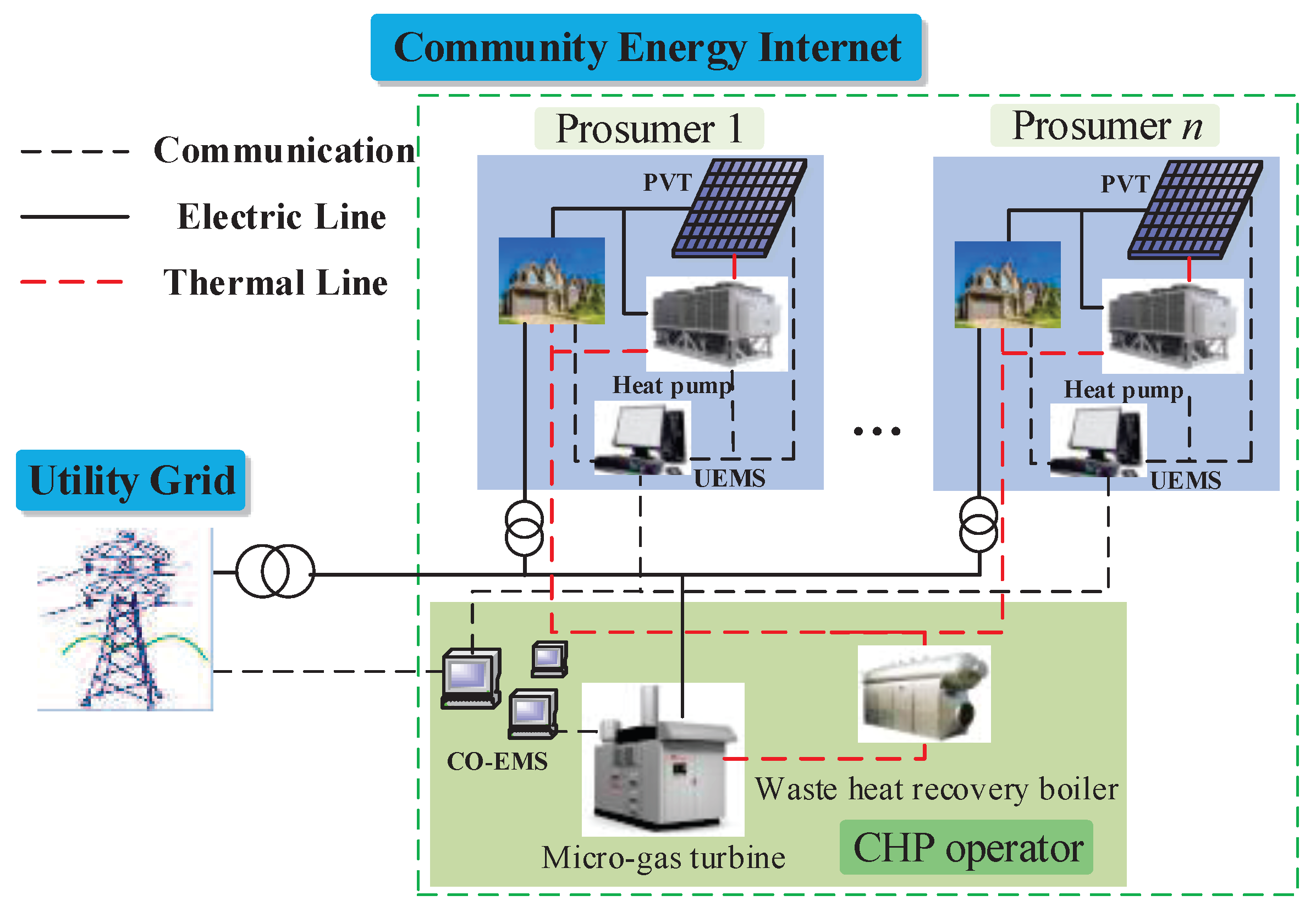
The system architecture of the CEI is shown in Figure 1. There are three entities: PVT-HP prosumer, CHP operator and utility grid. Each prosumer is equipped with PVT, heat pump and user energy management system (UEMS) [13]. UEMS is in charge of communicating with other entities, adjusting local load demand and determine the output of heat pump. The heat pump uses the water from the tank of PVT system as the low temperature heat resource to produce high temperature hot water for end users. Excess electric and thermal energy can be shared among prosumers and the electricity can be sold to utility grid as well. CHP operator guarantees thermal supply through recovering the waste heat of micro-gas turbine when the heat pump cannot meet the users’ thermal demand and conducts trading with utility grid and prosumers inside the community. Its energy management system is CHP operator energy management system (CO-EMS). After using the self-produce and CHP power, if the CEI is still in lack of electricity, the insufficient can be balanced by the utility grid.
3. Basic Knowledge of Consensus Algorithm
In this section, the notations of graph theory and two consensus protocols are presented.
3.1. Graph Theory
Consider a CEI with N PVT-HP prosumers, a CHP operator and utility grid. A directed connected graph is used to represent the communication topology of the CEI, where V is the node set and is the edge set. The prosumers set, CHP operator set and utility grid set are expressed as , and , respectively. A directed edge from i to j is denoted by an ordered pair , which means that if and only if (iff) node j can receive messages from node i. The in-neighbors of the ith node is denoted by and is the cardinality of in-neighbor set of node i. Similarly, the out-neighbors of the node is denoted by and is the cardinality of out-neighbor set of node i. Since it is obvious that node i can obtain its own state information, each node belongs to both its in-neighbor and out-neighbor set, i.e., as well as [24]. It is worth noting that the communication network is strongly connected, i.e., any two nodes have directed path between them.
3.2. Consensus Protocols
CHP can produce electric and thermal power while PVT-HP prosumer can act as a producer or a consumer according to the load level, output power of PV and heat pump. Besides, the deviated electric power is balanced by the utility grid. Thus, the network is divided into electric network and thermal network, i.e., the electric network set and the thermal network set and note that . Let us define two stochastic matrices named row stochastic matrix and column stochastic matrix associated with the electric network of N nodes as follows:
Similarly, and are the stochastic matrices of thermal network of M nodes:
For simplicity, the electric network is taken as an example for the following part. It is assumed that denotes the state vector of all nodes in the electric network at iteration k. For the initial value , the following two lemmas will be helpful for the design of consensus algorithm [24].
Lemma 1.
(Consensus): If the network is strongly connected, for the discrete consensus algorithm , there holds that , where c is a constant.
Lemma 2.
(Ratio Consensus): If the network is strongly connected, for the discrete consensus algorithm , there holds that , where is the element of the unit eigenvector corresponding to eigenvalue 1 of the matrix S.
4. System Model
4.1. Profit of Utility Grid
When the CEI is in lack of electric power, utility grid purchases the electricity from the power plant (i.e., coal-fired generation) to meet the demand of the end users. On the contrary, if there is plenty of solar energy, CEI can feed the excess power back to the utility grid to get income. Hence, the cost of utility grid at time t can be denoted as:
where is the net electric power of the CEI at time t, are the cost coefficients of the power plant, is the unit price of PV energy selling to the utility grid.
It’s assumed that the cost function of utility grid should be continuous, here is set as 0 in Equation (3). For the convenience of calculations, the piecewise function of utility grid can be approximated by a quadratic function by referring to [10]:
Therefore, for the utility grid i, , the profit can be expressed as:
where is the profit of utility grid, is the electric price at time slot t in CEI, is the electricity selling to the CEI.
4.2. Utility of Prosumer
Generally, a PVT-HP prosumer can get revenue through trading energy with utility grid, CHP operator and other prosumers, which means that the utility function of a prosumer should consider the profit of selling energy and the cost of purchasing energy firstly. For prosumer i, , its profit or cost at each time slot is defined as:
where is the profit (positive) or cost (negative) of a prosumer at time slot t, is the thermal price at time slot t, is the load demand of electric power, is the electric power consumed by the heat pump, is the predicted electric power of PVT system, is the load demand of thermal power, is the thermal power produced by the heat pump.
For the heat pump, it uses the water from the tank of PVT system as the low temperature heat resource to produce high temperature hot water. The thermal power produced by the heat pump is denoted by:
where is the coefficient of performance of the heat pump.
Moreover, from the perspective of DR, the prosumers adjust their usage of energy motivated by the prices, and then get financially benefit. Simultaneously, adjusting the prosumer’s load profiles would cause uncomfortable [33] or inconvenience [10] impact. Thus, the equivalent negative cost on the utility of prosumers can be defined as follows.
where , are the coefficients of inconvenience and uncomfortable, respectively; and are the initial electric power and thermal power consumption, respectively.
From Equation (8), the negative impact of DR increases with the deviation of power consumption, both on electricity and heat. Hence, for prosumer i, , its profit function at each time slot can be updated as follows:
4.3. Profit of CHP
CHP produces electric power as well as thermal power leading to a high overall efficiency, its profit function is represented as [11]:
where , , , , , are the cost coefficients of CHP system.
The heat-to-electric rate of CHP may be different due to the variable load conditions. CHP can operate either in the Following Thermal Load (FTL) mode or in the Following Electric Load (FEL) mode. For CHP i, , the coupling model of thermal and electric is denoted by [34]:
where is the electric efficiency, is the heat recovery rate of heat recovery boiler, and is the coupling coefficient between heat and electricity.
When the load rate of CHP is less than 30%, its electric efficient will be much lower, so we only start the CHP unit when its load rate is greater than 30%:
where is the rated power of CHP unit and it is assumed that the electric efficient is a constant when the load rate of CHP is over 30%.
5. Problem Formulation and Algorithm
5.1. Optimization Problem
In the energy market of the CEI, prosumers, utility grid and CHP operator compete with each other to maximize its own interests for their selfishness. To guarantee both efficiency and fairness, social welfare maximization is introduced and widely used. Social welfare maximization ensures the overall interests and maximizes each individual interest simultaneously. Here, we add up all the profits or utilities of the participants as the social welfare:
At any time, the electric power and thermal power should be balanced in practical operation.
Based on the previous description, energy management of the CEI can be formulated as a convex optimization problem:
where the equality constraints are global power constraints which describes the electric power balance and thermal power balance, the inequality constraints are local power constraints for all the participants, and are the lower and upper limit of electric power, and are the lower and upper limit of thermal power, respectively.
5.2. Problem Decoupling
To resolve the convex optimization problem with consensus algorithm, we need to decouple the global constraints. The Lagrangian multiplier method is a typical approach to transfer the equality constraints to the objective function. The corresponding Lagrangian function of original problem is given by:
where , and = and , are the Lagrange multipliers at time t that are introduced to decouple the global power constraints.
There exist different global constraints between electric network and thermal network and leading to the separation of them. We define as incremental cost (incremental utility) for the energy sources (the demand) i in electric network as follows:
Similarly, the incremental cost (incremental utility) for the energy sources (the demand) i of thermal network is given by:
From Equations (20)–(22), we can decouple the primal problem into 3 sub-optimization problems only with local constraints.
Prosumer subproblem ():
Utility grid subproblem ():
CHP subproblem ():
Now, all the subproblems only have local constraints to be solved, which are appropriate to use consensus algorithm in a directed communication network.
5.3. Design of Algorithm
The local electric and thermal power mismatches are denoted as and , respectively. and represent the gain parameters. The final errors , and , are for the power mismatch and incremental cost (utility). To simplify the description of algorithm, t is omitted in the following part, i.e., denotes . The detail of the algorithm can be found in Algorithms 1 and 2.
| Algorithm 1 Algorithm for participants in the CEI |
|
| Algorithm 2 Iteration Process |
| While true |
|
For Algorithm 1, in Initialization, the value of , , , and can be set to any valid value. Please note that the initial value of should be when for the PV energy is preferentially self-consumed.
For Algorithm 2, first, the convergence of both incremental cost (utility) and local power mismatch are guaranteed by the update rules Equations (35) and (36) which are derived from Lemma 1. Second, the thermal and electric power are calculated based on the updated according to Equations (37)–(43). Third, each participant updates its own local power mismatch based on the updated power according to Equations (44) and (45) that come from Lemma 2. Fourth, the iteration breaks until all the approach to the same value and the total power mismatch get close to 0. By choosing a small enough value for , , the iterative procedure finally converges to the global optimum.
6. Case Study
6.1. Basic Data
In this paper, a CEI comprises 6 residential buildings is choosed as the study case and each building represents a PVT-HP prosumer. The parameters of utility grid, CHP and PVT-HP prosumer are listed in Table 1. All the load data are collected from the smart residential buildings of demonstration projects in Beijing [33]. The settings of the case study are consistent with these projects to make the method capable of the practical applications. The daily curves of electric, thermal load, and electric net power are shown in Figure 2 and the range of load adjustment is set between −20% and +20%. Figure 2 shows the daily load profiles and PV energy curve of the CEI. Figure 2a is the daily electric load profiles of six prosumers, the peak loads appear at 20:00. Figure 2b is the daily thermal load profiles of six prosumers. With the change of temperature, end users need more heat at night. By equipping with PVT systems, end users utilize the solar energy to meet part of the electric load and thermal load from 8:00 to 20:00. Therefore, the electric net power has shown negative values from 12:00 to 16:00. , , and are set as 0.000595, 0.000555, 0.01 and 0.01, respectively.
6.2. Results of Simulation
6.2.1. Convergence and Optimality of Consensus Algorithm
In this section, we apply the proposed model in the CEI and use MATLAB (2014a, The MathWorks, Inc, Natick, MA, USA) to programme for testing the convergence and optimality of Algorithm 2. The iterative optimization processes of incremental cost (incremental utility) , the local power of each participator and the local thermal power mismatch at 1:00 are shown in Figure 3. As shown in Figure 3a, the incremental cost (incremental utility) converges to its final value = 0.2701 CNY/kWh with iterations, while all the local thermal power mismatch approach to 0.0098 as shown in Figure 3b. Moreover, from Figure 3c, the results show that the output power of CHP is 0 kW at the beginning and then gradually approaches to the convergence value = 17.01 kW. The net thermal power of prosumer 1 and prosumer 2 are negative which means that they share excess thermal energy with other prosumers. More importantly, all the prosumers and CHP operator achieve the same incremental cost (incremental utility), under which all the participants achieve their own goal, i.e., maximize the individual welfare.
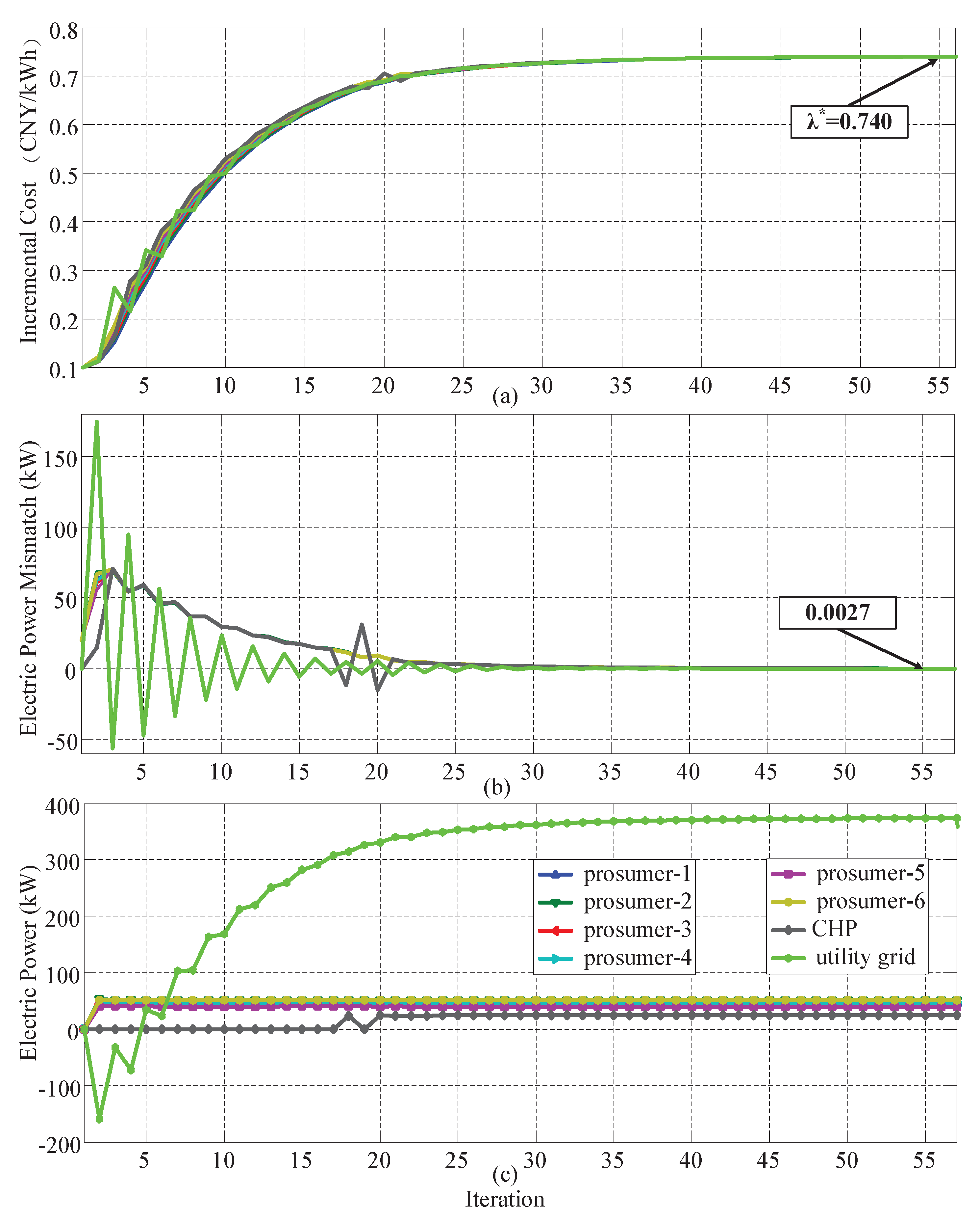
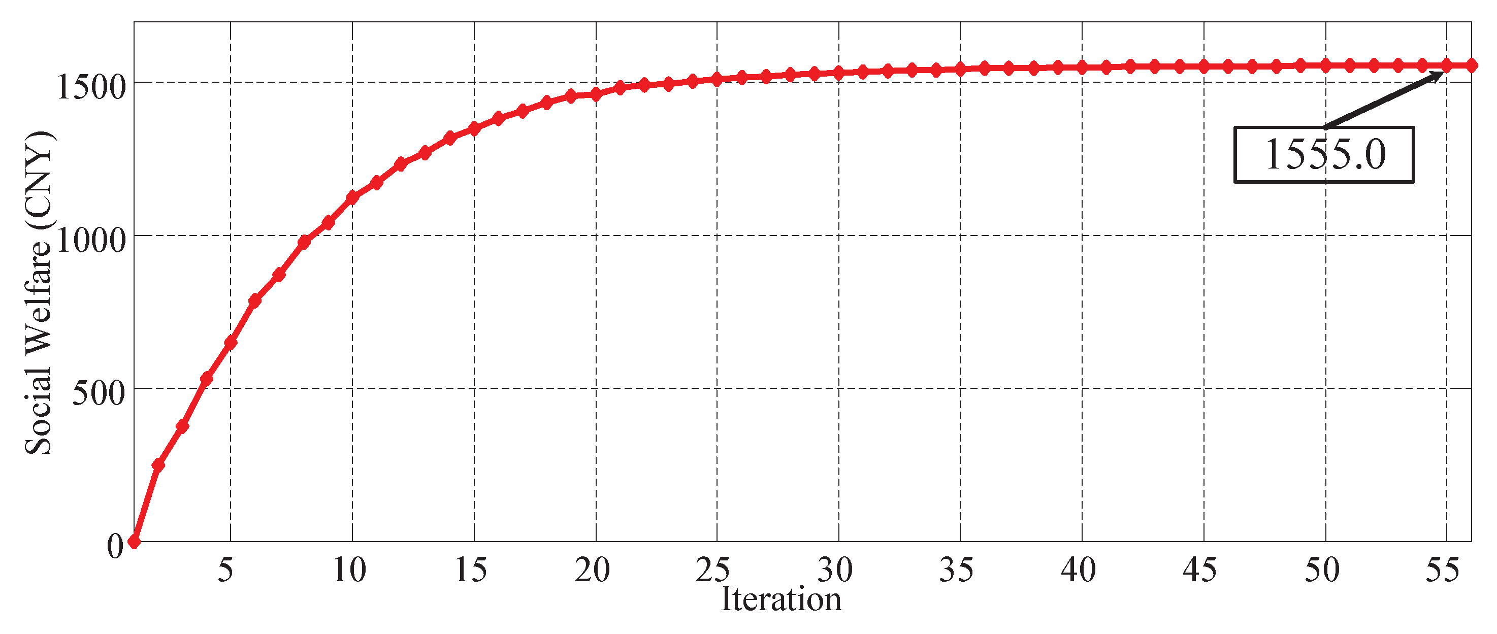
Figure 4 shows the convergence results of electric network. In Figure 4a,b, all the participants convergence to the same incremental cost (utility), i.e., = 0.740 CNY/kWh, while the local power mismatch get close to 0.0027. Moreover, Figure 4c shows that the variation tendency of CHP is the same as the results in Figure 3c. In this time slot, there is no solar energy, the prosumers has to buy 373.46 kWh from the utility grid to meet the electric demand of load and heat pump. The total social welfare of the CEI approaches to its convergence result at CNY, as shown in Figure 5.
6.2.2. Results of Price and Net Power
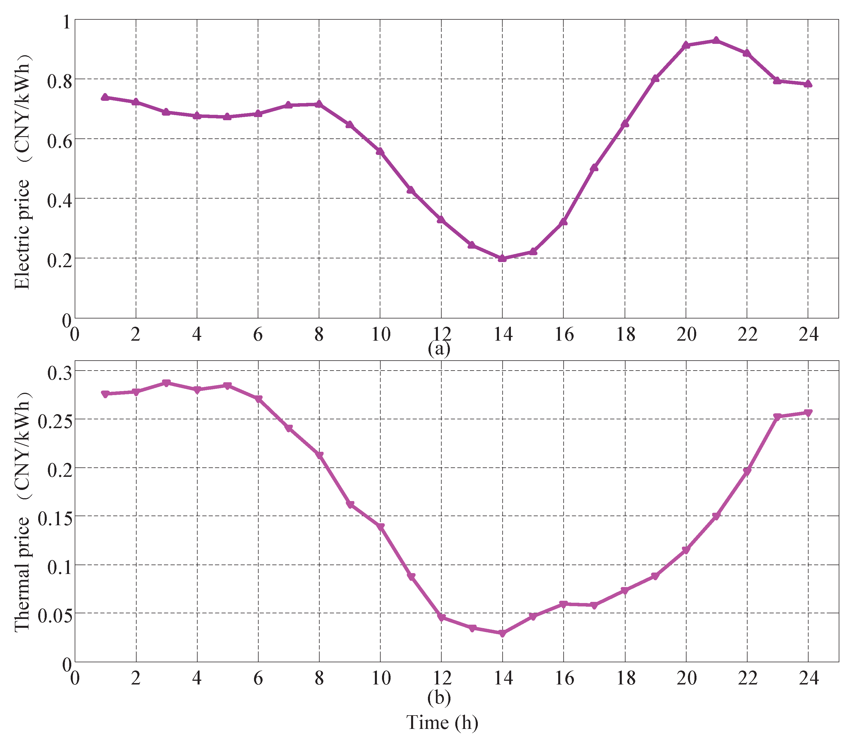
By using the basic data of six prosumers, CHP and utility grid, consensus-based energy sharing of the CEI on each time slot of a day can be solved by executing Algorithm 1. The price of electric power and thermal power during the daytime are shown in Figure 6. From 0:00 to 8:00 and 20:00 to 24:00, the electric price is high because there is no solar energy and the end users have to purchase energy from the utility grid. The electric price changes with the variety of PV output from 8:00 to 20:00 and gets its minimal value 0.1973 CYN/kWh at 14:00. After 20:00, the electric price increases for the reason that there is a peak electric load from 19:00 to 22:00. The variation tendency of the thermal price is consistent with the thermal load curve. At night, the higher thermal load level leads to the higher prices, i.e., 0.25–0.3 CNY/kWh. The thermal price decreases with the thermal load reduction and increases gradually with the increasing demand during the day.
The net power of each prosumer, CHP and utility grid can be seen in Figure 7. As shown in Figure 7a, the net thermal power of prosumers 4–6 are positive which means they are always a thermal consumer during the day and prosumers 1–3 can act as a thermal producer or a thermal consumer alternatively. Especially, from 10:00 to 17:00, as a thermal producer, prosumers 1–3 share their excess thermal energy to prosumers 4–6. During the time, the heat pump of each prosumer makes full use of the abundant solar energy to produce high temperature thermal energy to meet the load demand. The CHP is stopped during 9:00–17:00 to increase the economic effectiveness because the load rate is less than 30%. Moreover, Figure 7b shows the net electric power of each prosumer. From 12:00 to 16:00, there are plenty of solar energy and all the prosumers act as a electric producer to sell electric energy to utility grid.
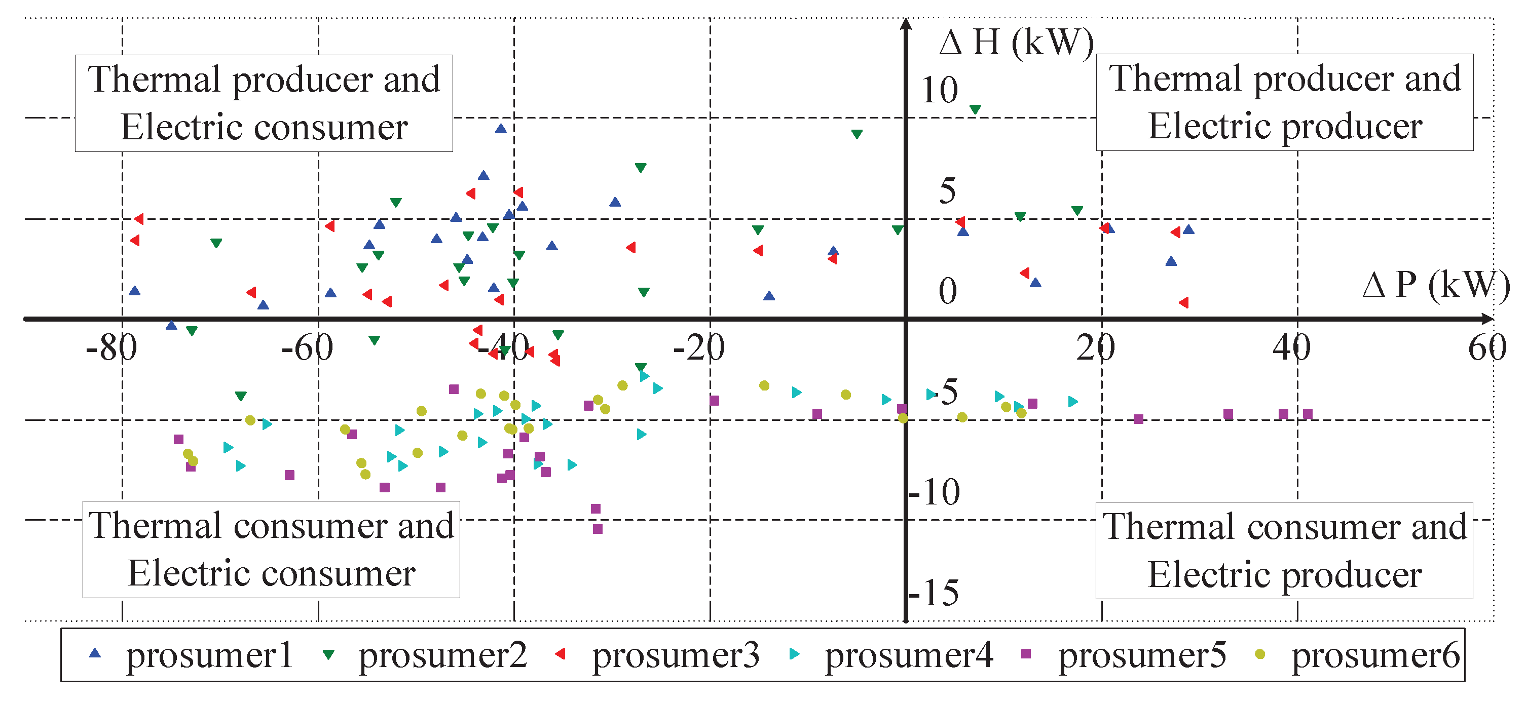
By using the results of each time slot, an interesting result can be found that there are four types of role attributes for PVT-HP prosumers. That is, in one time slot, a thermal producer can be an electric consumer, and a thermal consumer can also be acted as an electric producer, which can be further shown in Figure 8. The horizontal axis represents electric net power while the vertical axis represents the thermal net power.
The results show that the number of prosumer roles acted as electric producer is much less than the number of electric consumer. This is mainly due to the fact that the solar electric power is only excess during the periods 12:00–16:00 of daytime. In contrast, the roles of thermal producers and consumers are distributed evenly in the vertical axis, because the capacity of heat pump is matched with the load demand.
6.3. Analysis of Computation Time and Applications
With the development of smart grid, the user side has gradually been equipped with smart meters, building energy management system, as well as high speed Internet connections, which lay the hardware foundation of the consensus algorithm applications. Figure 3 and Figure 4 show the Algorithm 2 can approach the optimum solution in 55 iterations. According to the designed Algorithm 2 in Section 5.3, only increment cost (utility) and local power mismatch are exchanged between participants at each iteration which is presented in Equations (35), (36), (44) and (45). Each participant broadcasts its value of last iteration while receives data from neighboring participants. Therefore, there are about 2 Bytes data broadcasted and 14 Bytes data received in one iteration for a participant, the total data exchange for the hour-ahead optimization is less than 110 Bytes (broadcasted) and 770 Bytes (received). If we use the LTE 230 MHZ VPN network for data exchange, the latency of each message is less than 3 s (average 2 s). Furthermore, we use a computer with Intel Core i5-4570 CPU 3.2 GHz (Intel, Santa Clara, CA, USA), 8G memory (Samsung Corporation, Seoul, Korea), and MATLAB 2014a as the time cost testing environment for the algorithm. The average computation time is 0.037 s for one iteration, combined with the communication latency, the maximum time cost of the hour-ahead optimization is about 2.78 min (average 1.87 min). Thus, the optimal scheduling of the CEI can be start at 5 min prior to the energy sharing. As mentioned above, the consensus algorithm is bound to be a good distributed algorithm in future energy management system.
7. Conclusions
In this paper, we have proposed a consensus-based energy sharing method for solving social welfare problem of the CEI. From the results of case study, we have shown that all the increment costs (utilities) convergence to a same value while the power balance is satisfied, which means that all participants achieve their own maximal profits and the social welfare maximization problem has been solved. Furthermore, if the capacity of PVT and heat pumps are properly configured and the capacity of heat pump can meet the demand of thermal load, which means the heat pump can make full use of the waste heat of PVT, the prosumers can make full use of solar energy to guarantee the thermal power balance and reduces the installed capacity of CHP. It is an interesting result that a thermal producer can be an electric consumer and a thermal consumer can also act as an electric producer in the market of the CEI. In practical work, the sun’s illumination has a greater impact on the system. The energy storage devices are to be an useful tool to solve the problem. Therefor, we will take the storage system into account in our future work.
Author Contributions
The paper was a collaborative effort between the authors. N.L., B.G., Z.L., Y.W. contributed collectively to the theoretical analysis, modeling, simulation and manuscript preparation.
Funding
This work was supported in part by the National Natural Science Foundation of China under Grant 51577059 and in part by the Fundamental Research Funds for the Central Universities under Grant 2018ZD13.
Conflicts of Interest
The authors declare no conflict of interest.
References
- Rifkin, J. The third industrial revolution: How lateral power is transforming energy, the economy, and the world. Survival 2011, 2, 67–68. [Google Scholar] [CrossRef]
- Wang, K.; Yu, J.; Yu, Y.; Qian, Y.; Zeng, D.; Guo, S.; Xiang, Y.; Wu, J. A Survey on Energy Internet: Architecture, Approach, and Emerging Technologies. IEEE Syst. J. 2017. [Google Scholar] [CrossRef]
- Sabbah, A.I.; El-Mougy, A.; Ibnkahla, M. A Survey of Networking Challenges and Routing Protocols in Smart Grids. IEEE Trans. Ind. Inform. 2013, 10, 210–221. [Google Scholar] [CrossRef]
- Bui, N.; Castellani, A.P.; Casari, P.; Zorzi, M. The internet of energy: a web-enabled smart grid system. IEEE Netw. 2012, 26, 39–45. [Google Scholar] [CrossRef]
- Huang, A.Q.; Crow, M.L.; Heydt, G.T.; Zheng, J.P.; Dale, S.J. The Future Renewable Electric Energy Delivery and Management (FREEDM) System: The Energy Internet. Proc. IEEE 2010, 99, 133–148. [Google Scholar] [CrossRef]
- Huang, A. FREEDM system—A vision for the future grid. In Proceedings of the 2010 IEEE Power and Energy Society General Meeting, Providence, RI, USA, 25–29 July 2010; pp. 1–4. [Google Scholar]
- Ji, Z.; Sun, Y.; Wang, S.; Zhao, J. Design of a three-phase cascaded Power Electronic Transformer based on energy Internet. In Proceedings of the International Conference on Sustainable Power Generation and Supply, Hangzhou, China, 8–9 September 2012; pp. 1–6. [Google Scholar]
- Arnold, M.; Negenborn, R.R.; Andersson, G.; Schutter, B.D. Distributed Predictive Control for Energy Hub Coordination in Coupled Electricity and Gas Networks; Springer: Berlin, Germany, 2010; pp. 235–273. [Google Scholar]
- Rastegar, M.; Fotuhi-Firuzabad, M. Load Management in a Residential Energy Hub with Renewable Distributed Energy Resources. Energy Build. 2015, 107, 234–242. [Google Scholar] [CrossRef]
- Ma, L.; Liu, N.; Wang, L.; Zhang, J.; Lei, J.; Zeng, Z.; Wang, C.; Cheng, M. Multi-party energy management for smart building cluster with PV systems using automatic demand response. Energy Build. 2016, 121, 11–21. [Google Scholar] [CrossRef]
- Liu, N.; Wang, J.; Wang, L. Distributed energy management for interconnected operation of combined heat and power-based microgrids with demand response. J. Mod. Power Syst. Clean Energy 2017, 5, 478–488. [Google Scholar] [CrossRef] [Green Version]
- Liu, N.; Yu, X.; Wang, C.; Li, C.; Ma, L.; Lei, J. Energy-Sharing Model With Price-Based Demand Response for Microgrids of Peer-to-Peer Prosumers. IEEE Trans. Power Syst. 2017, 32, 3569–3583. [Google Scholar] [CrossRef]
- Liu, N.; Chen, Q.; Liu, J.; Lu, X.; Li, P.; Lei, J.; Zhang, J. A Heuristic Operation Strategy for Commercial Building Microgrids Containing EVs and PV System. IEEE Trans. Ind. Electron. 2015, 62, 2560–2570. [Google Scholar] [CrossRef]
- Radziemska, E. The effect of temperature on the power drop in crystalline silicon solar cells. Renew. Energy 2003, 28, 1–12. [Google Scholar] [CrossRef]
- He, W.; Chow, T.T.; Ji, J.; Lu, J.; Pei, G.; Chan, L.S. Hybrid photovoltaic and thermal solar-collector designed for natural circulation of water. Appl. Energy 2006, 83, 199–210. [Google Scholar] [CrossRef]
- Huang, B.J.; Lin, T.H.; Hung, W.C.; Sun, F.S. Performance evaluation of solar photovoltaic/thermal systems. Sol. Energy 2014, 70, 443–448. [Google Scholar] [CrossRef]
- Putrayudha, S.A.; Kang, E.C.; Evgueniy, E.; Libing, Y.; Lee, E.J. A study of photovoltaic/thermal (PVT)-ground source heat pump hybrid system by using fuzzy logic control. Appl. Therm. Eng. 2015, 89, 578–586. [Google Scholar] [CrossRef]
- Tsai, H.L. Modeling and validation of refrigerant-based PVT-assisted heat pump water heating system. Sol. Energy 2015, 122, 36–47. [Google Scholar] [CrossRef]
- Emmi, G.; Tisato, C.; Zarrella, A.; Carli, M.D. Multi-Source Heat Pump Coupled with a Photovoltaic Thermal (PVT) Hybrid Solar Collectors Technology: a Case Study in Residential Application. Int. J. Energy Prod. Manag. 2016, 1, 382–392. [Google Scholar]
- Bertram, E.; Glembin, J.; Rockendorf, G. Unglazed PVT collectors as additional heat source in heat pump systems with borehole heat exchanger. Energy Procedia 2012, 30, 414–423. [Google Scholar] [CrossRef]
- Liang, Y.; Liu, F.; Wang, C.; Mei, S. Distributed demand-side energy management scheme in residential smart grids: An ordinal state-based potential game approach. Appl. Energy 2017, 206, 991–1008. [Google Scholar] [CrossRef]
- Pipattanasomporn, M.; Feroze, H.; Rahman, S. Multi-agent systems in a distributed smart grid: Design and implementation. In Proceedings of the 2009 IEEE/PES Power Systems Conference and Exposition (PSCE ’09), Seattle, WA, USA, 15–18 March 2009; pp. 1–8. [Google Scholar]
- Shi, W.; Xie, X.; Chu, C.C.; Gadh, R. Distributed Optimal Energy Management in Microgrids. IEEE Trans. Smart Grid 2015, 6, 1137–1146. [Google Scholar] [CrossRef]
- Zhang, Z.; Chow, M.Y. Convergence Analysis of the Incremental Cost Consensus Algorithm Under Different Communication Network Topologies in a Smart Grid. IEEE Trans. Power Syst. 2012, 27, 1761–1768. [Google Scholar] [CrossRef]
- Elsayed, W.T.; El-Saadany, E.F. A Fully Decentralized Approach for Solving the Economic Dispatch Problem. IEEE Trans. Power Syst. 2015, 30, 2179–2189. [Google Scholar] [CrossRef]
- Yang, S.; Tan, S.; Xu, J.X. Consensus Based Approach for Economic Dispatch Problem in a Smart Grid. IEEE Trans. Power Syst. 2013, 28, 4416–4426. [Google Scholar] [CrossRef]
- Binetti, G.; Davoudi, A.; Lewis, F.L.; Naso, D.; Turchiano, B. Distributed Consensus-Based Economic Dispatch With Transmission Losses. IEEE Trans. Power Syst. 2014, 29, 1711–1720. [Google Scholar] [CrossRef]
- Zhao, C.; He, J.; Cheng, P.; Chen, J. Consensus-Based Energy Management in Smart Grid With Transmission Losses and Directed Communication. IEEE Trans. Smart Grid 2017, 8, 2049–2061. [Google Scholar] [CrossRef]
- Wu, D.; Yang, T.; Stoorvogel, A.A.; Stoustrup, J. Distributed Optimal Coordination for Distributed Energy Resources in Power Systems. IEEE Trans. Autom. Sci. Eng. 2017, 14, 414–424. [Google Scholar] [CrossRef]
- Xing, H.; Lin, Z.; Fu, M.; Hobbs, B.F. Distributed algorithm for dynamic economic power dispatch with energy storage in smart grids. IET Control Theory Appl. 2017, 11, 1813–1821. [Google Scholar] [CrossRef]
- Asr, N.R.; Zhang, Z.; Chow, M.Y. Consensus-based distributed energy management with real-time pricing. In Proceedings of the 2013 IEEE Power and Energy Society General Meeting, Vancouver, BC, Canada, 21–25 July 2013; pp. 1–5. [Google Scholar]
- Meng, W.; Wang, X. Distributed Energy Management in Smart Grid With Wind Power and Temporally Coupled Constraints. IEEE Trans. Ind. Electron. 2017, 64, 6052–6062. [Google Scholar] [CrossRef]
- Liu, N.; He, L.; Yu, X.; Ma, L. Multiparty Energy Management for Grid-Connected Microgrids With Heat- and Electricity-Coupled Demand Response. IEEE Trans. Ind. Inform. 2018, 14, 1887–1897. [Google Scholar] [CrossRef]
- Wang, J.; Sui, J.; Jin, H. An improved operation strategy of combined cooling heating andpower system following electrical load. Energy 2015, 85, 654–666. [Google Scholar] [CrossRef]
Figure 1.
Structure of Community Energy Internet (CEI) with photovoltaic-thermal and heat pump (PVT-HP) prosumers.
Figure 1.
Structure of Community Energy Internet (CEI) with photovoltaic-thermal and heat pump (PVT-HP) prosumers.

Figure 2.
Daily load curves of prosumers: (a) daily electric load curves; (b) daily thermal load curves; (c) daily electric net power curves.
Figure 2.
Daily load curves of prosumers: (a) daily electric load curves; (b) daily thermal load curves; (c) daily electric net power curves.
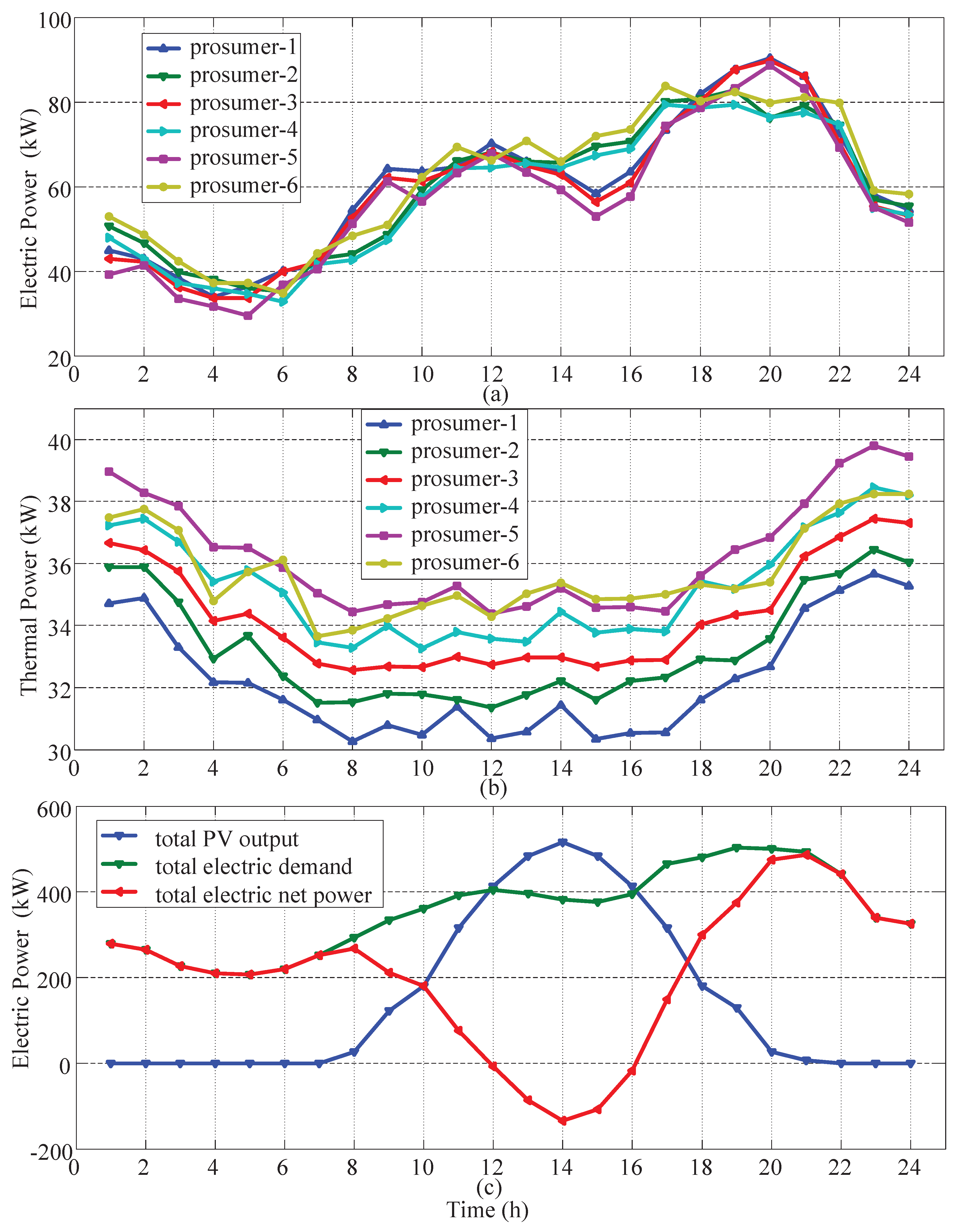
Figure 3.
Convergence results of thermal network: (a) incremental cost (utility); (b) local thermal power mismatch; (c) local generated or consumed thermal power.
Figure 3.
Convergence results of thermal network: (a) incremental cost (utility); (b) local thermal power mismatch; (c) local generated or consumed thermal power.
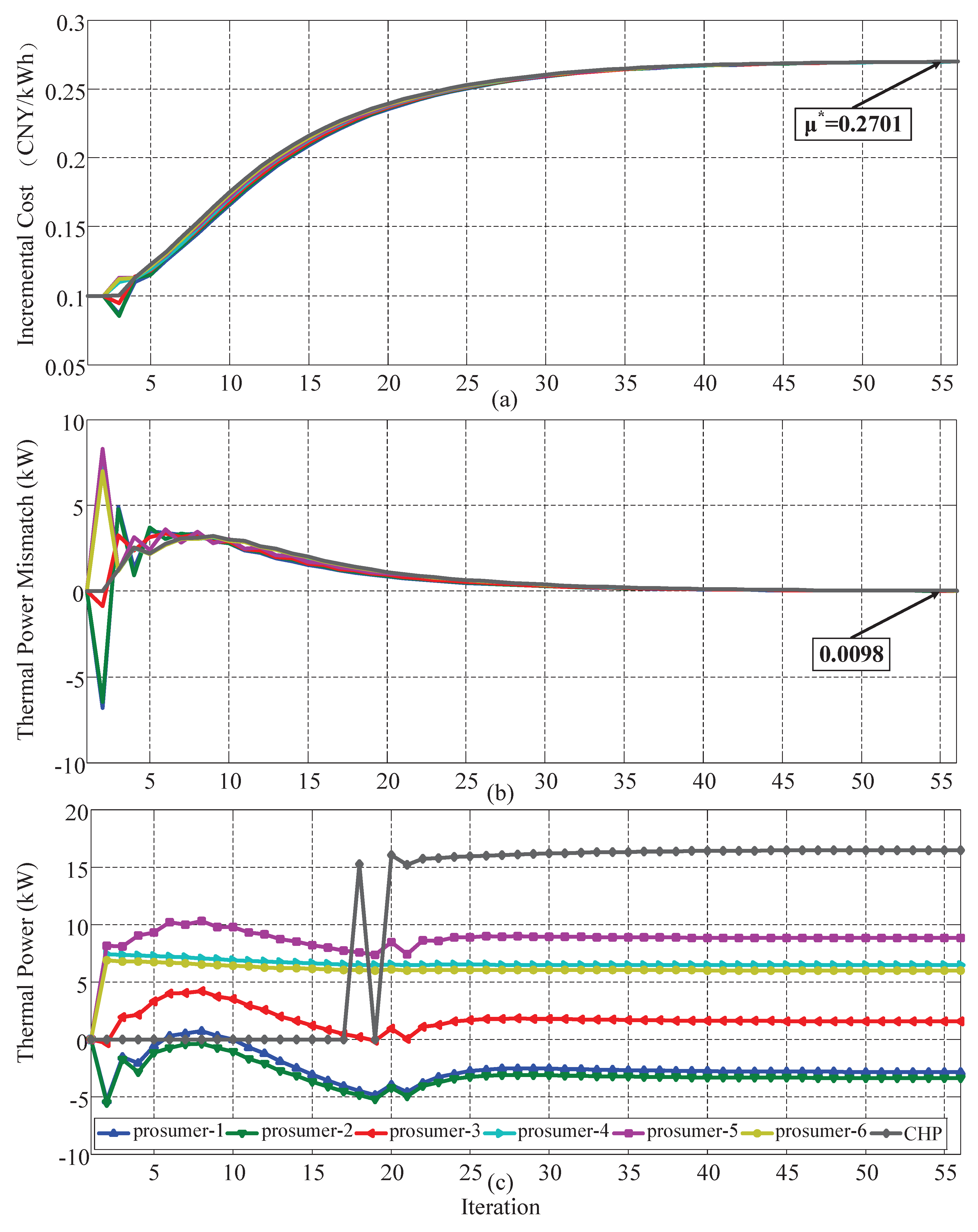
Figure 4.
Convergence results of electric network: (a) incremental cost (utility); (b) local electric power mismatch; (c) local generated and consumed electric power.
Figure 4.
Convergence results of electric network: (a) incremental cost (utility); (b) local electric power mismatch; (c) local generated and consumed electric power.

Figure 5.
Convergence results of total social welfare.

Figure 6.
(a) Electric price and (b) thermal price during the daytime.

Figure 7.
Net power during the day. (a) Net thermal power; (b) Net electric power.
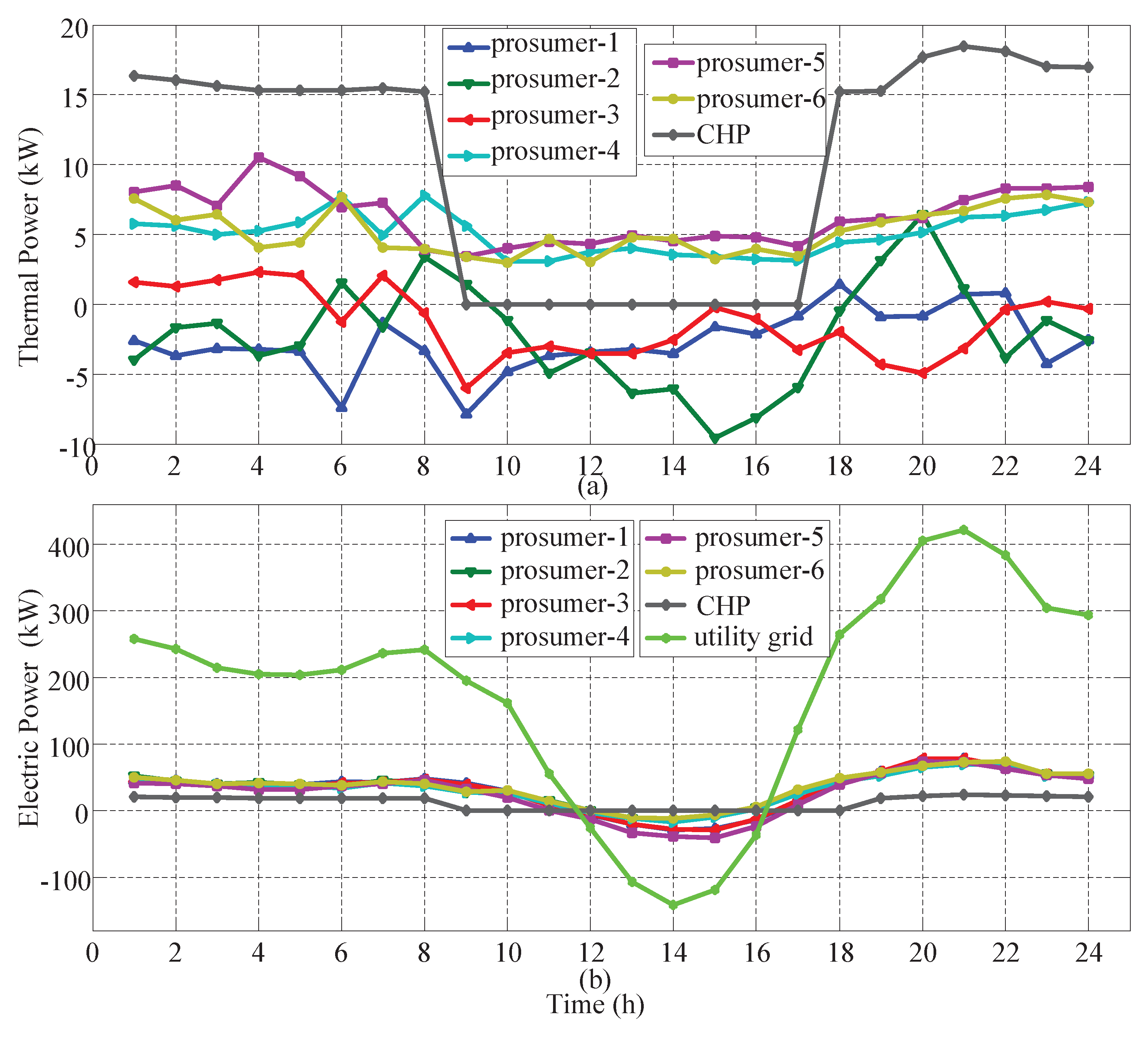
Figure 8.
Roles of prosumer during the day.


Table 1.
Parameters of participants.
| Participant | Parameters | Value |
|---|---|---|
| Utility grid | Cost coefficients | a = 0.00059, b = 0.302, c = 0 |
| Capacity | [−500, 1000] (kW) | |
| CHP | Cost coefficients | = 0.03395, = 4.6425, = 0.00442 |
| = 1.345, = 0.00384, = 0.004 | ||
| Efficiency | = 0.3441, = 0.80 | |
| Capacity | 50 (kW) | |
| PVT-HP prosumer | COP | 3 |
| Coefficients of comfort | (0.03–0.055), (0.025–0.1) | |
| Capacity of heat pump | 15 (kW) |
© 2018 by the authors. Licensee MDPI, Basel, Switzerland. This article is an open access article distributed under the terms and conditions of the Creative Commons Attribution (CC BY) license (http://creativecommons.org/licenses/by/4.0/).
Share and Cite
MDPI and ACS Style
Liu, N.; Guo, B.; Liu, Z.; Wang, Y. Distributed Energy Sharing for PVT-HP Prosumers in Community Energy Internet: A Consensus Approach. Energies 2018, 11, 1891. https://doi.org/10.3390/en11071891
AMA Style
Liu N, Guo B, Liu Z, Wang Y. Distributed Energy Sharing for PVT-HP Prosumers in Community Energy Internet: A Consensus Approach. Energies. 2018; 11(7):1891. https://doi.org/10.3390/en11071891
Chicago/Turabian StyleLiu, Nian, Bin Guo, Zifa Liu, and Yongli Wang. 2018. "Distributed Energy Sharing for PVT-HP Prosumers in Community Energy Internet: A Consensus Approach" Energies 11, no. 7: 1891. https://doi.org/10.3390/en11071891
Note that from the first issue of 2016, this journal uses article numbers instead of page numbers. See further details here.