Analysis of the Variability of Wave Energy Due to Climate Changes on the Example of the Black Sea


Shirshov Institute of Oceanology of Russian Academy of Sciences, Moscow 117997, Russia
*
Author to whom correspondence should be addressed.
Energies 2018, 11(8), 2020; https://doi.org/10.3390/en11082020
Submission received: 25 June 2018
/
Revised: 2 August 2018
/
Accepted: 2 August 2018
/
Published: 3 August 2018
(This article belongs to the Special Issue Wave and Tidal Energy)
Abstract
:An analysis of the variability of wave climate and energy within the Black Sea for the period 1960–2011 was made using field data from the Voluntary Observing Ship Program. Methods using wavelet analysis were applied. It was determined that the power flux of wave energy in the Black Sea fluctuates: the highest value is 4.2 kW/m, the lowest is 1.4 kW/m. Results indicate significant correlations among the fluctuations of the average annual wave heights, periods, the power flux of wave energy, and teleconnection patterns of the North Atlantic Oscillation (NAO), the Atlantic Multi-decadal Oscillation (AMO), the Pacific Decadal Oscillation (PDO) and the East Atlantic/West Russia (EA/WR). It was revealed that, in positive phases of long-term periods of AMO (50–60 years) as well as PDO, NAO, and AO (40 years), a decrease of wave energy was observed; however, an increase in wave energy was observed in the positive phase of a 15-year period of NAO and AO. The positive phase of changes of EA/WR for periods 50–60, 20–25, and 13 years led to an increase of wave energy. The approximation functions of the oscillations of the average annual wave heights, periods, and the power flux of wave energy for the Black Sea are proposed.
1. Introduction
Currently, numerous opportunities for renewable natural energy sources, such as wind and wave energy, are being widely discussed. The energy obtained from natural sources is environmentally friendly because it does not require the creation of special production cycles that often can pollute the environment, especially the atmosphere. For example, a unique wave energy plant was constructed in the harbor of a small fishing village Mutriku at the Basque Atlantic coastline.
To convert wave energy into electricity, special wave energy converters (WEC) are under development and are the subjects of significant research. A review of technologies which extract wave energy, an overview of wave energy potential, and the wave energy cost can be found in Rusu and Onea [1]. They have shown that the global wave power resources are 2.11 ± 0.05 TW [2].
At the same time, the distribution of wave power resources is nonhomogeneous in the World Ocean. Therefore, for the implementation of projects on wave energy use, an analysis of the available local wave energy potential is required. Traditionally, the energy potential estimations of different parts of the World Ocean are performed by modeling waves based on wind reanalysis; for example, studies by Atan and Goggins [3] and Soares et al. [4] discuss the Atlantic.
The Black Sea is an inland sea connected to the Mediterranean Sea by the Bosporus Strait. Its resources, including possible wave energy, have the great economic importance for the countries on its shores, such as Russia, Turkey, Georgia, Ukraine, Bulgaria, and Romania. For the Black Sea, such estimations for the all water area for periods 1900–2010 and 1990–2014 was conducted by Galabov [5], Rusu [6], and Divinsky and Kosyan [7]. The analysis for the wave energy potential along the southeastern coastline for the period 1995–2004 was performed in studies by Akpınar and Kömürcü [8,9].
Variability in the global climate can lead to changes in the wave climate. Recent studies have shown that a variability of climate is reflected in fluctuations in large-scale atmospheric circulation. These fluctuations are determined by so-called teleconnection patterns, for example, the North Atlantic Oscillation (NAO), the Atlantic Multi-decadal Oscillation (AMO), the Pacific Decadal Oscillation (PDO), the Arctic Oscillation (AO), and the East Atlantic-Western Russia pattern (EA/WR). Changes of teleconnection patterns can be described by corresponding climatic indices. Many studies have demonstrated the influence of these climatic indices on the variability of regional storminess, including the region of Black Sea [10,11,12,13,14,15,16,17]. For example, periods of wave climate variability for a 4–10 period were associated with fluctuations of the North Atlantic Oscillation, and a decrease in storms in the 2000s as associated with the low-frequency variability of the East Atlantic-Western Russia teleconnection pattern [11,13]. Long-term fluctuations (40–50 years) of maximum annual wave heights were identified in Polonsky et al. [12], and it was shown that fluctuations can be associated with changes of the Atlantic Multi-decadal and Pacific Decadal Oscillations.
Therefore, for wave energy extraction projects, it is necessary to know the regularities and trends of long-term changes of wave climates as well as their connection with global climate change. Notably, as a result of time-consuming computational costs and insufficient accuracy of wind reanalysis on large time scales, wave energy estimations are often made on time scales of 10–35 years and poorly reproduce fluctuations of long-term periods [18].
Meanwhile, as has been shown in Galabov [5], the modelling data obtained using different wind reanalysis may lead to significantly different estimates of wave energy for the same regions of the Black Sea. Accordingly, estimations for the average annual wind power flux for the entire Black Sea have varied considerably in recent studies, calculated at 3 kW/m in Akpınar and Kömürcü [9], 6–7 kW/m in Aydoğan et al. [19], and about 3–4 kW/m in Divinsky and Kosyan [7]. The maximum decadal average wave power of the Black Sea for 110 years (1900–2010) fluctuated from 2.7 kW/m to 3.3 kW/m during the period 1941–1950 and then decreased to 2.7 kW/m in the 2000s. Notably, wave energy fluctuations can be connected with variability in both the AMO and PDO indices [5].
In Divinsky and Kosyan [7], on the basis of modelling data analyses, the western part of the Black Sea was determined to be more energetic, especially the southwest, where the maximum wave power energy flux can reach 8–10 kW/m; in contrast, the eastern part is less energetic, about 2–4 kW/m. At the same time, for the northwestern Black Sea, average annual wave power energy flux was estimated to be about 4 kW/m [20]. The average annual wave power energy flux estimates made by Galabov [5] for the southwestern part of the Black Sea did not exceed 3 kW/m and fluctuated from 1.5 to 4 for the period 1900–2010.
Obviously, both the accuracy of the wave models and wind reanalysis data and the length of the time interval over which such estimates are made should influence wave energy estimates, especially if there is long-term climate variability of the wave data. To avoid the inaccuracies mentioned above, it would be better to use the data of field observations and to know the main periods of climatic variability of the Black Sea. However, detailed analysis of periods of variability of the wave climate for the Black Sea have not been conducted. Therefore, the main goal of this work is to analyze the wave climate variability of the Black Sea on the basis of long-term field observations data, to identify the main periods of climatic variability, and to make estimates of the possible variability of wave energy in connection with climate change.
2. Data and Methods of Analysis
A significant problem in analysing the variability of the wave climate, especially those of low-frequency, is the wave data of field observations. Wave data are available in a very limited volume, which usually belongs to national hydrometeorological services. The observation stations are located on the shore; therefore, the wave heights are recorded predominantly in the coastal zone of the sea. Concurrently, there are no data of continuous long-term (more than 20 years), full-scale field instrumental observations of the waves. Therefore, for field wave data, we will use the database from the Voluntary Observing Ship Program (VOS). More details about these observations are available at [21]. The database contains meteorological observations, including the visual registration of heights of waves and wave periods carried out by ships on a voluntary basis during sea and ocean routes. On the base of limited collections of VOS data the widly used wave statistics atlas for marine officers and naval engineers were developed [22].
One potential weakness in visual wave observations is that they are less reliable than, for example, satellite or model data because of their low accuracy due to human factor, space-time inhomogeneity, as well as some difficulties with preprocessing and bias corrections. Despite the quantitative discrepancies in estimations of wave heights which have been noted by many researchers (up to 40%), when these estimations are compared with model data and buoys measurements [23,24,25], these discrepancies largely relate to comparisons of monthly observations. When comparing mean annual data, accuracy is significantly increased, and, as noted in Gulev et al. [25], for the majority of locations, observational uncertainties are within 20% of mean values, which is sufficient for climatological studies. Notably, the accuracy of comparing VOS data with other instrumental measurements depends on the number of measuring stations in a given region: the more measuring stations, the less the discrepancy in the estimation of wave heights. Accuracy also depends on the preprocessing of VOS data [26]. The precision of modern measurements of wave heights and periods is comparable to visual observations, as shown in Grigorieva et al. [27,28] and summarized in Table 1, which is provided by Grigorieva and compiled on the basis of her analysis of wave data of National Data Buoy Center (https://www.ndbc.noaa.gov) and altimetry data of GlobWave project (http://www.globwave.org). As seen in Table 1, VOS data are comparable with the data of direct instrumental measurements and present several advantages. Moreover, in the VOS data, the parameters of wind driven sea waves and swell are recorded separately.
On the basis of the VOS data in the Shirshov Institute of Oceanology of Russian Academy of Sciences, the Wave Atlas was developed [29]. Because this relies on visual observation data, it is necessary to control a quality of records for the detection of “bugs” and other potential inaccuracies. For the Wave Atlas, the following preprocessing of VOS data was made: artificial errors correction or elimination, correction of small wave heights, examination of extreme wave heights, and inconsistency of wave parameters, etc. Black Sea VOS data from the Wave Atlas for wave heights are available for period 1948–2011. However, records of wave heights and periods are only available from 1960. Accordingly, the wave data of the wind-driven sea with the wave steepness (ratio of height to wavelength) less than 0.1 for the period 1960–2011 years were selected for analysis, which resulted in a total of 85,061 records.
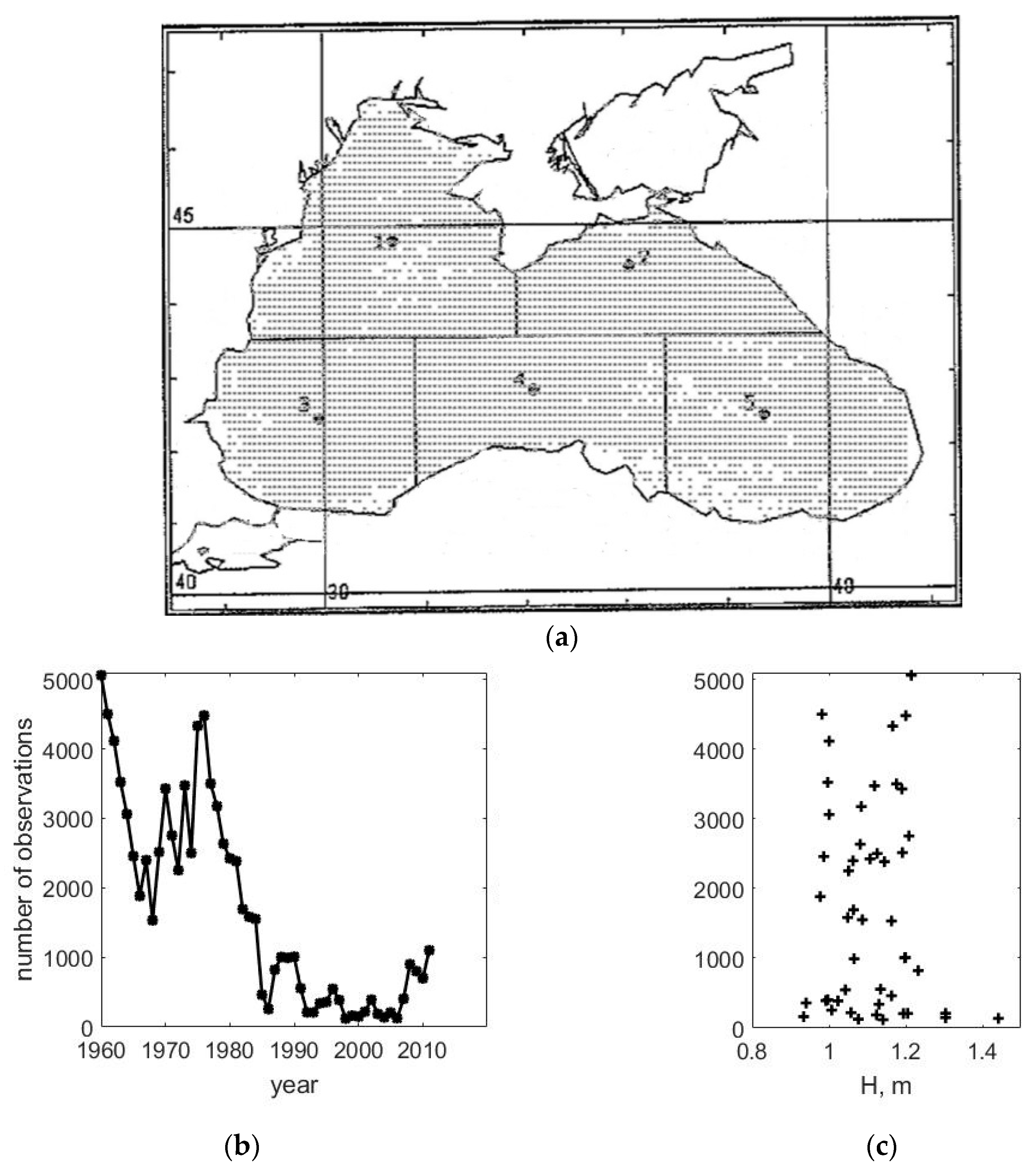
The distribution of observation points along the Black Sea, the density of observation data for different regions, the total number of observations per year, and the dependence of the average annual wave height on the number of observations are shown in Figure 1. The density of observation data for the period 1960–2011 for the five main regions of the sea includes: region 1—18,364 observations, region 2—11,762, region 3—31,132, region 4—15,742, and region 5—7876. Clearly, in recent years, the number of observations has decreased (Figure 1b), but the average annual wave height is practically independent from the number of observations (Figure 1c).
The impact of global climate variability on the wave climate and wave energy will be estimated on the basis of an analysis of the relationships of the climatic indices (NAO, AO, AMO, PDO, EA/WR) with heights, periods, and energy of average annual waves. The values of dimensionless climatic indices, calculated by certain methods, were taken from the website of the National Oceanic and Atmospheric Administration of the USA [30].
Because the time series of analysed data is rather short (only 52 terms), to reveal the periodicity, the method of continuous wavelet transform with the Morlet wavelet function was used instead of a classical spectral analysis [31]. Wavelet transform is a type of scan of the investigated time series by frequencies that allows us to analyse the structure of non-stationary processes in time and to establish periodicity even in data containing an incomplete period of change. For a mutual correlation analysis, the method of wavelet-correlation developed earlier by the authors was applied instead of a classical correlation analysis [15,18]. Wavelet-correlations are the construction of a correlation function between the wavelet transforms of two signals and between the same wavelet-frequency bands. It is an analog of the correlation analysis, for which the original signals are preliminarily filtered on a multitude of narrow-band signals of characteristic frequency bands; subsequently, the correlations between these narrow-band signals are analyzed. If the number of such narrow-band signals is sufficiently large, then each such narrow-band signal can be considered as a quasi-stationary signal that enables an analysis of the correlation relations between two nonstationary processes.
For a detailed analysis of the structure of variability processes, the spavlet analysis (analysis of the spectra of modules of wavelet coefficients) was used [32]. A spavlet analysis is an analog of spectral analysis of the envelope of the signal. It allows for a determination of amplitude modulations of some frequency scales. To construct the spectra, we used parametric spectral analysis, also known as the Yule-Walker method.
3. Fluctuations of the Average Annual Wave Heights and Periods in Connection with the Changes of Climatic Indices
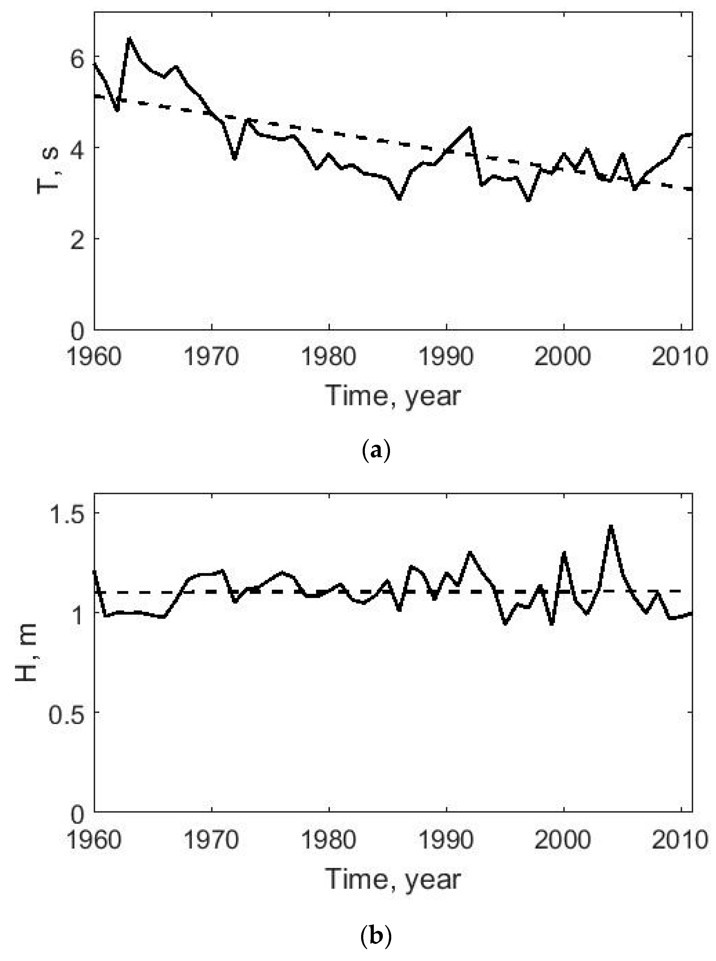
The changes of average annual wave heights and periods according to VOS data for the Black Sea from 1960 to 2011 are shown in Figure 2.
Clearly, there are inter-annual fluctuations of the average annual wave heights and periods. For wave heights, this variability increases in amplitude over the considered time period. However, the average annual wave height remains practically constant, about 1.1 m. For the period 1960–2011, the largest value of average annual waves is 1.4 m, with the smallest at 0.93 m. The average annual wave period decreases 0.04 s·year−1; the longest period is 6.4 s, with the shortest period at 3 s, and the average annual wave period for the considered 51 years is 4.1 s. It can be assumed that the change of the average annual wave period has a low-frequency periodicity: a sharp decrease was observed beginning in the 1960s and then a visible increase, starting approximately in 2005.
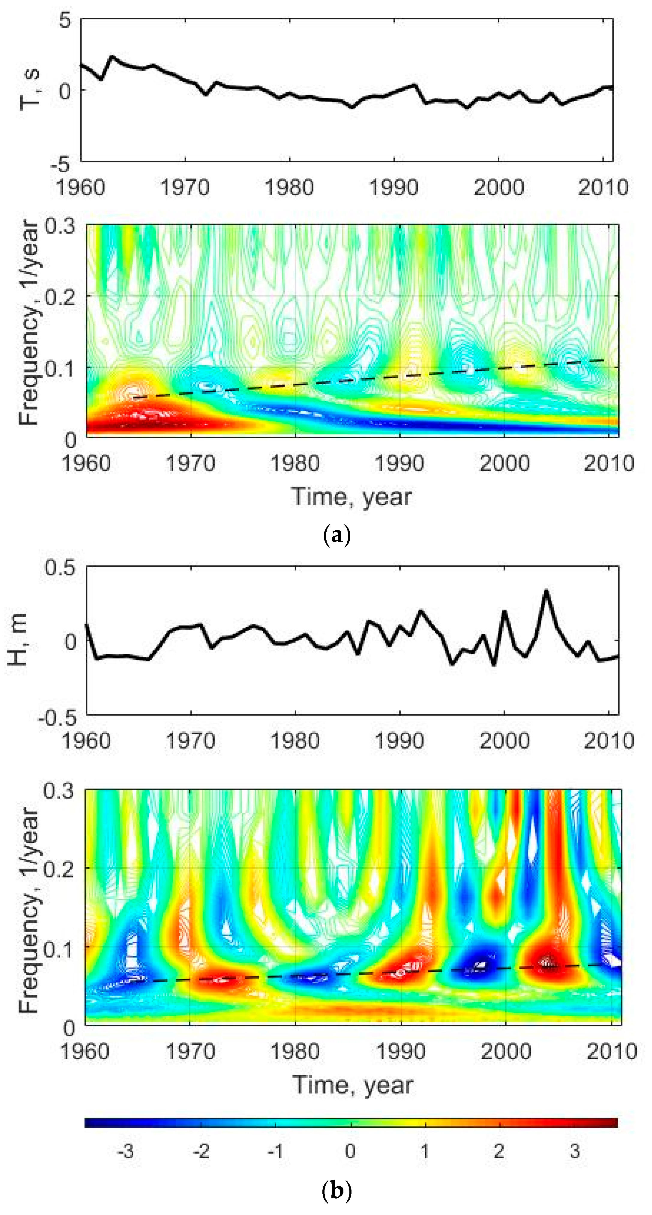
As wavelet analysis has shown, for the data of average annual wave periods, there is a periodic change on frequency scales of 0.015–0.02 year−1. Additionally, changes of the average annual period in the frequency range 0.05–0.13 year−1 are non-stationary. For example, the characteristic frequency scale of 0.07 year−1 increases with time to 0.1 year−1 (Figure 3a).
The changes of the average annual wave height are also non-stationary. For example, the characteristic frequency scale 0.05 year−1 has an increasing trend to 0.08 year−1. For frequency scales in the range 0.1–0.16 year−1, beginning in 1985, the frequency scale 0.1 year−1 increases to 0.16 year−1; after 1985, there are no trends and the frequency 0.16 year−1 is stable (Figure 3b).
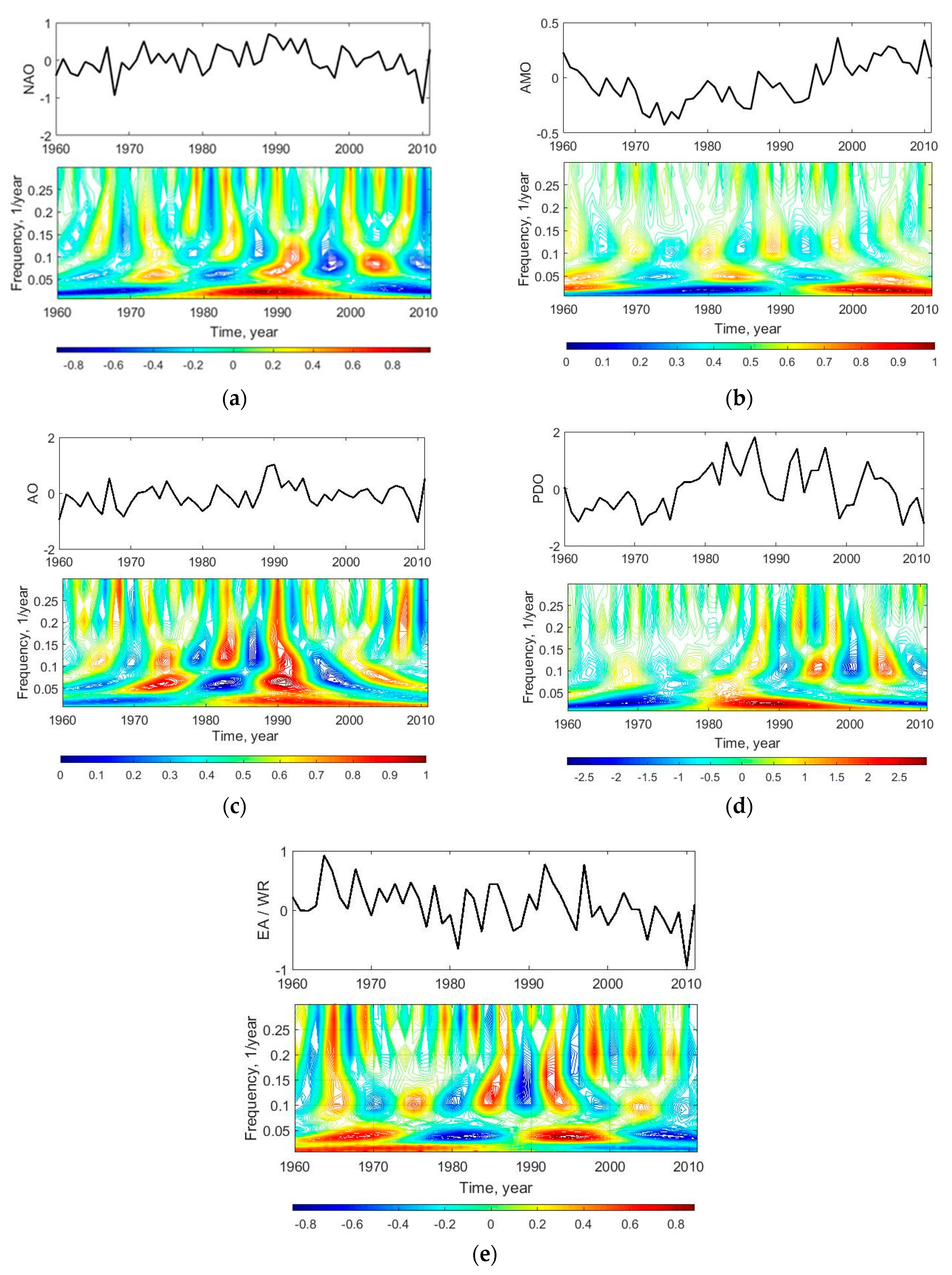
All data chosen for analysis climatic indices also changed to non-stationary. Figure 4 shows the wavelet transforms of all indices. According to the wavelet analysis, low-frequency oscillations of all indices can be identified. For AMO, the characteristic low frequencies are 0.022 and 0.05 year−1, for NAO—0.022 and 0.06 year−1, for PDO—0.025 year−1, for AO—0.026 and 0.06 year−1, and for EA-WR—0.035 and 0.1 year−1. Wavelet analysis shows that, for all climatic indices, there are different trends of frequencies changes in the range 0.09–0.13 and 0.2–0.3 year−1.
A visual comparison of the wavelet diagrams shows the similarity between the wavelet transforms of changes of NAO and the average annual wave heights, especially in the frequency range less than 0.16 year–1. Wavelet diagram of the changes of the average period are similar to wavelet diagrams of the changes seen in PDO and AMO. This similarity indicates the occurrence of an identical long-term (decadal and multi-decadal) periodicity of changes of average annual wave heights, periods, and corresponding climatic indices.
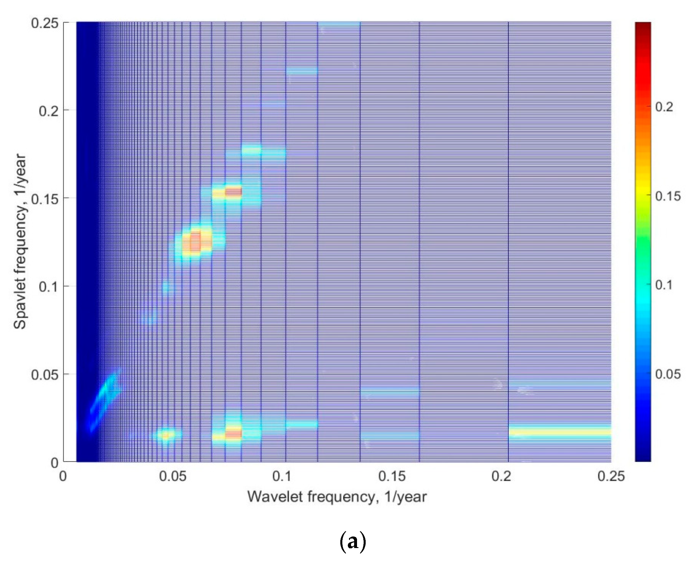
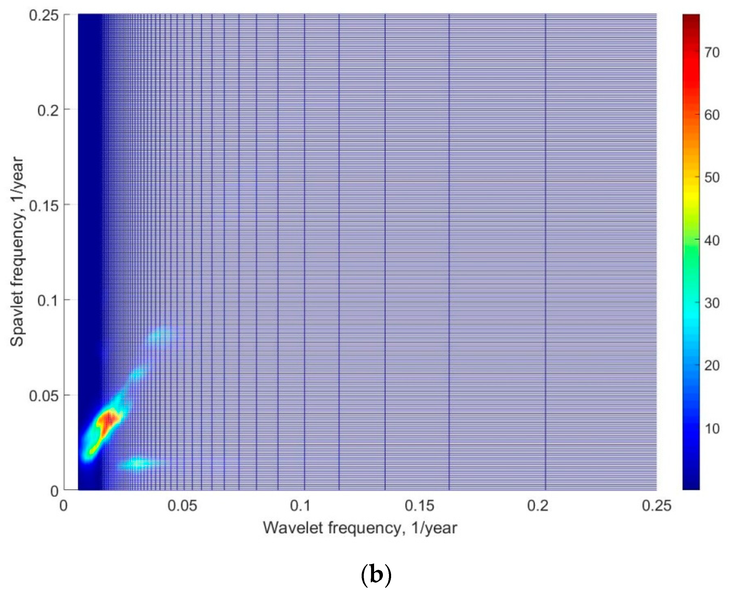
A detailed analysis of the structure of non-stationary processes of changes to average annual wave heights, periods, and climatic indices to identify a connection between them can conducted by a spavlet analysis. Spavlet is the set of spectra of the wavelet coefficient modules of each frequency scale of the wavelet transform [32]. The low-frequency components of the wavelet coefficients modules are an analog of the envelope of a narrow frequency band signal centered on the wavelet frequency of a given scale. The spectra were calculated by the Yule-Walker method of parametric spectral analysis for the best estimation of low-frequency components and period that are comparable with the duration of observations.
The spavlet analysis clearly shows the presence of low-frequency modulation, with a frequency of 0.016 year−1 and wavelet frequency scales of 0.05, 0.07–0.08, and 0.2–0.25 year−1 for average annual wave heights (Figure 5a). As seen in Figure 5a, the figure appears as a ridge parallel to the wavelet frequencies axis at spavlet′s frequency of 0.016 year−1. As seen in Figure 5, the ridge on the spavlet diagram at spavlet′s frequency equal to the double wavelet′s frequency is not significant because it was produced by the doubling of wavelets coefficients frequencies at the creation of its modules. The average annual period of waves is modulated by the same low frequency but only on a wavelet frequency of 0.03 year−1 (Figure 5b). On the basis of the structure of the spavlet, one can approximate functions for the process of periodicity of changes of average annual wave heights in the form:
FH(t) = A1cos(0.016t) + B1cos(0.016t)cos(0.05t) + C1cos(0.016t)cos(0.075t) + D1cos(0.016t)cos(0.22t),
And for the average annual wave periods as:
where coefficients A, B, C, and D should be determined empirically.
FT(t) = A2cos(0.016t) + B2cos(0.016t)cos(0.03t),
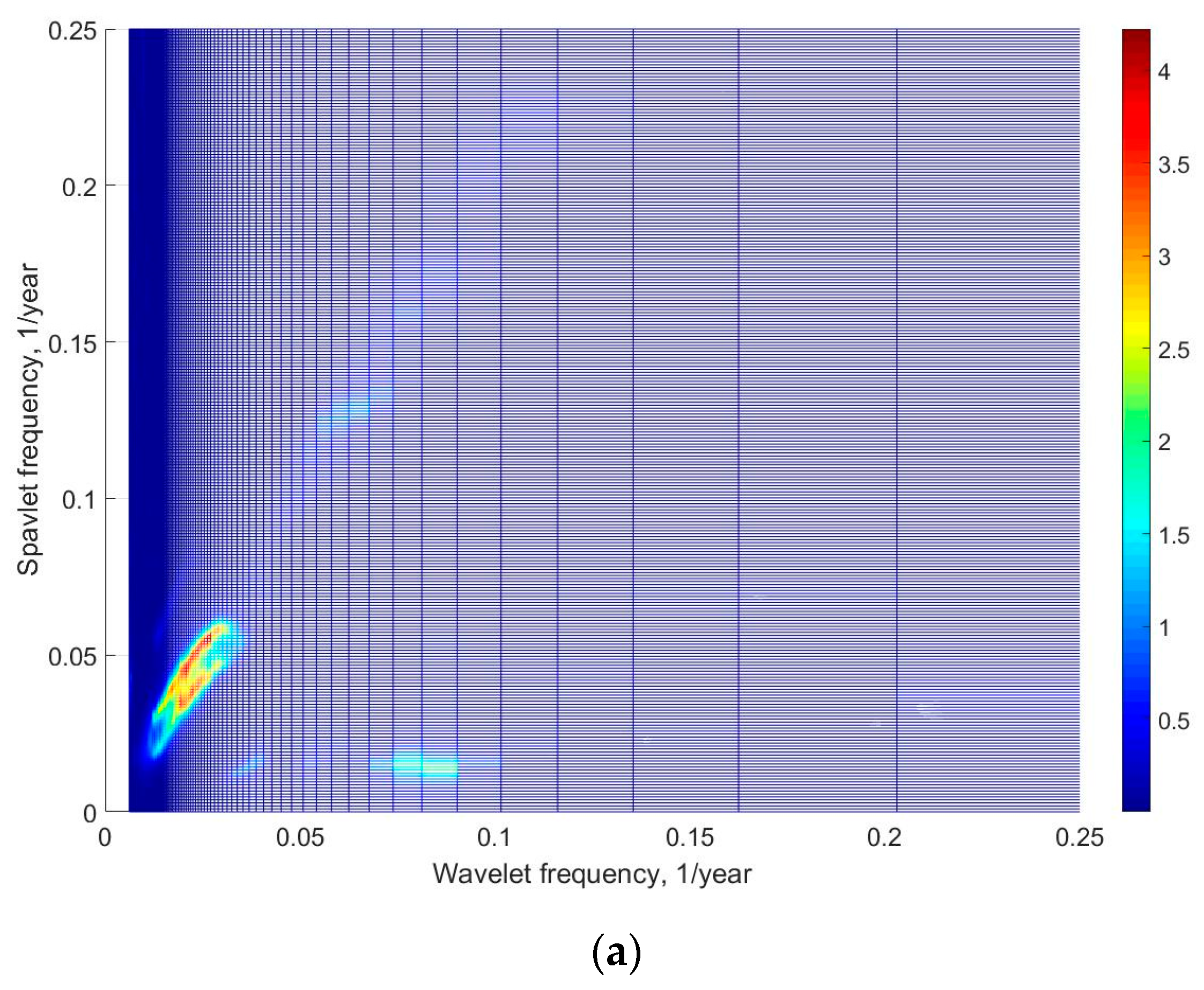
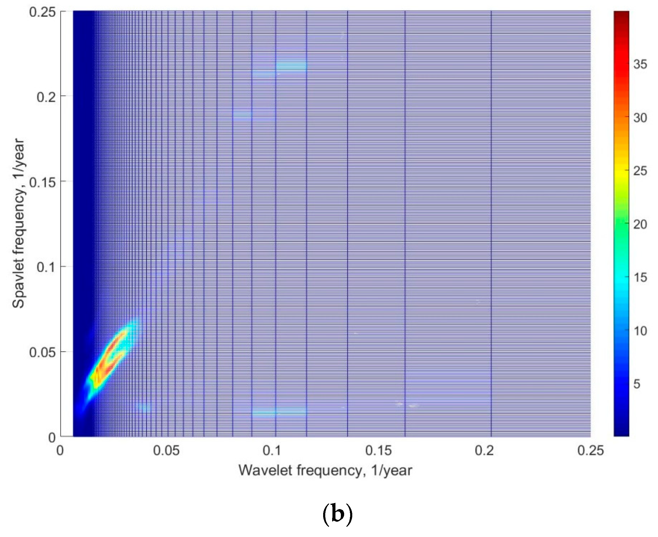
A spavlet analysis demonstrated that all climatic indices also have low-frequency modulations of wavelet frequencies in the range of 0.015–0.035 year−1. The fluctuations of average annual waves and the NAO index have the similar spavlet structures: the low-frequency modulation at a frequency of 0.016 year−1 of the main wavelet frequency scales 0.075 year−1 (Figure 5a and Figure 6a). In general, the spavlet structure of the fluctuations of the average annual wave period is similar to the structure of the PDO index: the low-frequency modulation by the frequency of 0.016 year−1 of the main wavelet frequency scales 0.03 year−1 (Figure 5b and Figure 6b).
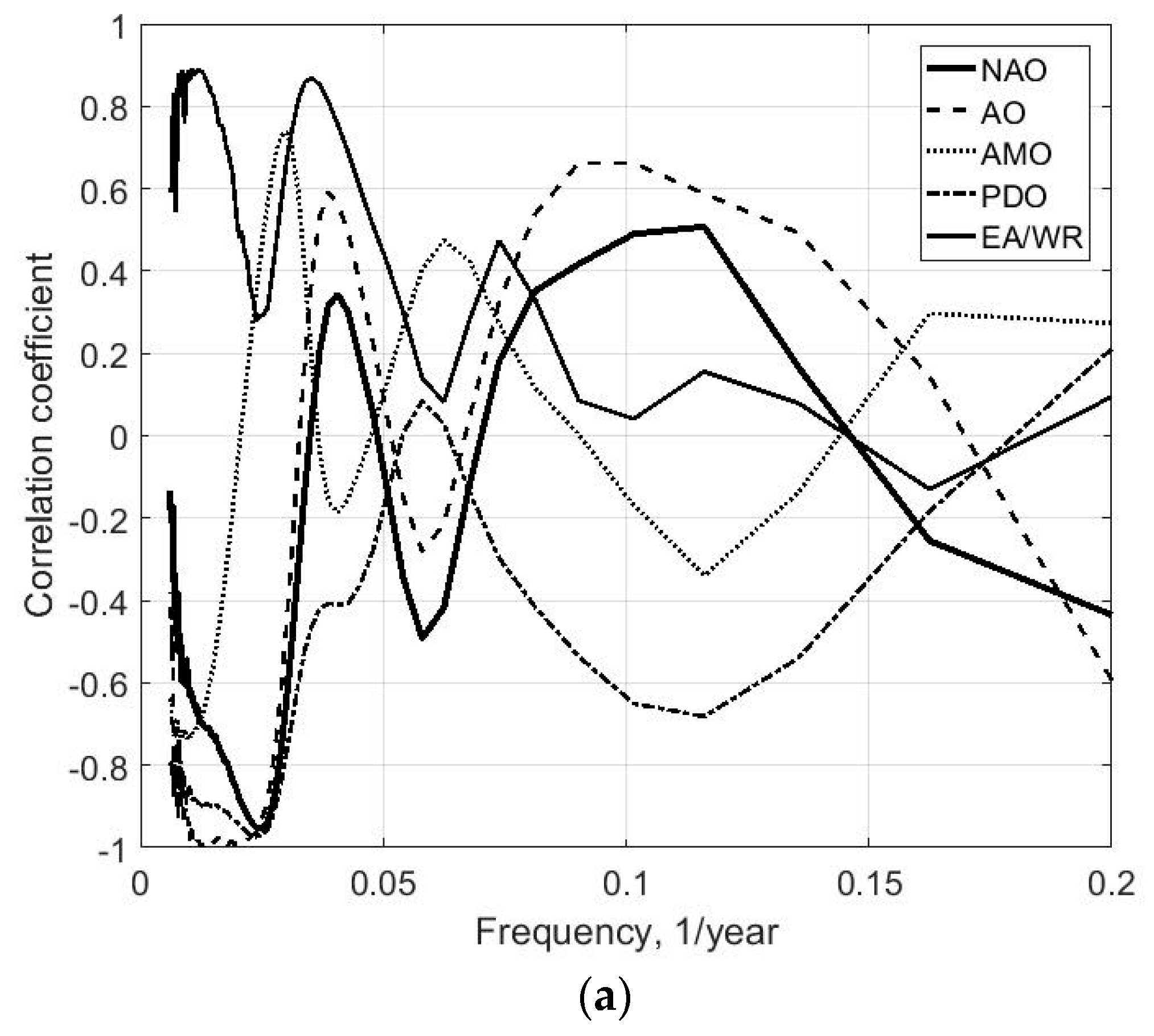
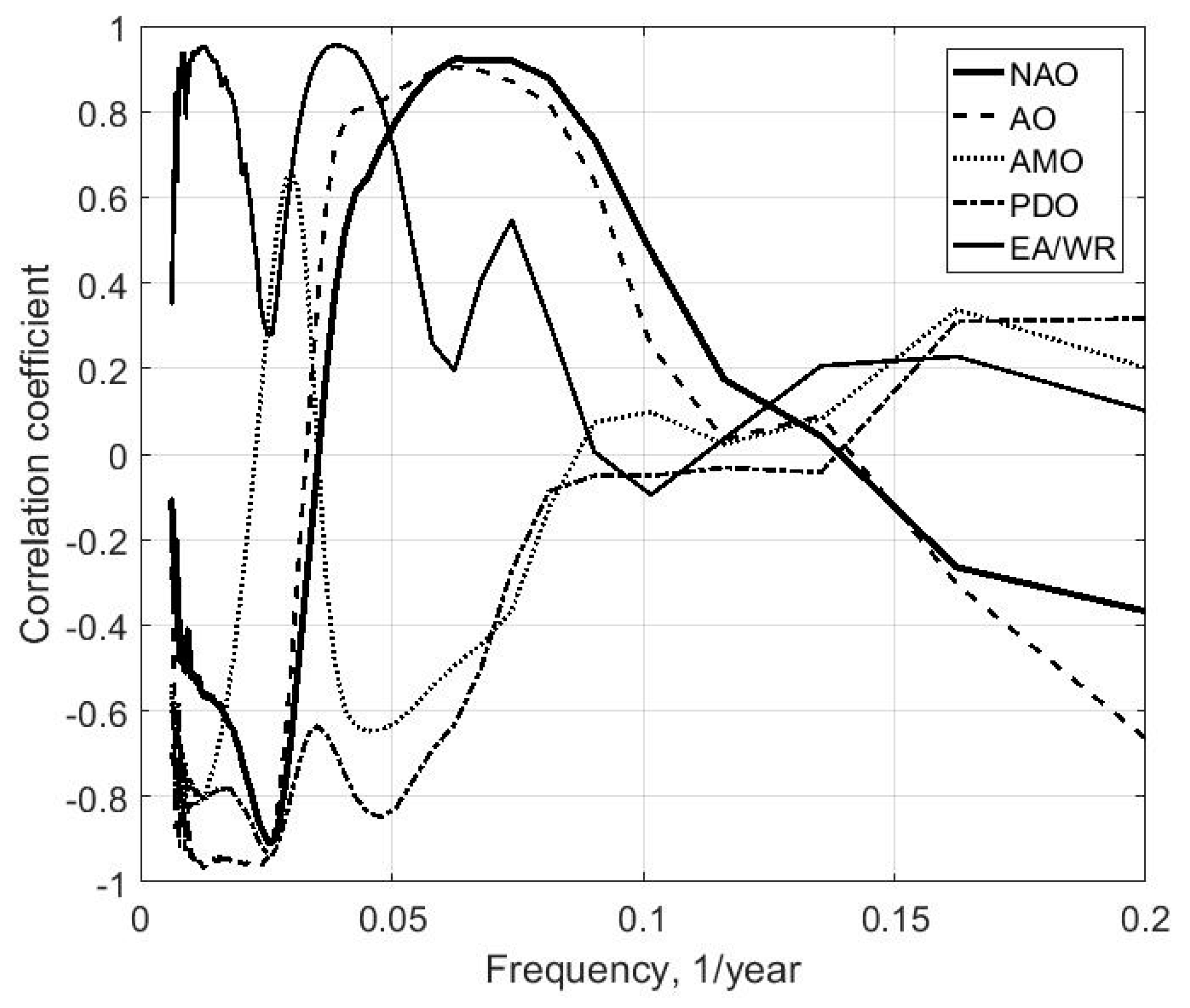
Because the changes in the wave heights, periods, and climatic indices are non-stationary, the classical correlation analysis to identify the correlation between them is inapplicable. Therefore, we propose to apply the wavelet-correlations method we developed in previous research [15,18], in which a correlation function between wavelet frequencies scales of wavelet transforms of two signals is constructed. In Figure 7, the frequency dependencies of the correlation coefficients between climatic indices and average annual wave heights and periods at zero time lags are presented.
Clearly, the changes of average annual wave heights and periods correlate well with the fluctuations of climatic indices, especially in the low-frequency range (multi-decadal and decadal periods). If we recalculate the frequencies in periods, then it is possible to identify subsequent periods of change to the average annual waves parameters in connection with the changes in climatic indices. The fluctuations of average annual wave heights are correlated with (1) NAO for periods of 40 and approximately 12–15 years; (2) AMO for periods of 30–35 years, 22, and 15 years; (3) PDO for periods of 40, 20, 8, and 6 years; (4) AO for periods of 40, 15, and 5 years; (5) EA/WR for periods of 30 and 13 years. The fluctuations of average annual wave periods are correlated with (1) NAO for periods of 40 and 10–12 years; (2) AMO for periods of 30–35 and 15 years; (3) PDO for periods of 40, 20, and 8 years; (4) AO for periods of 40, 25, 10, and 5 years; (5) EA/WR for periods of 30 and 13 years. In all cases, the values of the modulus of the correlation coefficient are more than 0.5.
According to the sign of correlation coefficients, the low-frequency fluctuations (periods more than 30 years) for the average annual wave heights occur in phase with NAO, PDO, and AO and in anti-phase with the AMO. Simultaneously, for the average annual wave periods, these fluctuations are the reverse: in phase with AMO and in anti-phase with NAO, PDO, and AO.
The largest correlation coefficients of the fluctuations of the average annual wave periods are those with changes in the PDO index and of the average annual wave heights, i.e., with the NAO index, which corresponds to the similarity of the structures of non-stationary processes revealed via a spavlet analysis.
Thus, long-term variability for both the average annual wave heights and periods can be associated with changes in PDO, AO, and NAO indices (for a 40-year period) and with AMO and EA/WR indices (i.e., periods of 30–35 years). Concurrently, there are periods of variability associated with AMO (15–16 years), PDO (8 years), and AO (5 years) indices. In the positive phase of the 40-year period of changes of the NAO, AO, and PDO, the average annual wave period decreases, but the average annual height increases. At the positive 30–35-year phase of AMO and EA/WR, the average annual wave period increases and the average annual wave height decreases. The average annual wave height also decreases in the positive phase of the 20-year period of change within PDO and AMO. The average annual wave height increases in the positive phase of NAO and AO changes during a period of 15 years. The average annual wave period will also increase in this positive phase of changes in the same indices but with a period of 10 years.
4. Fluctuations of the Power of Wave Energy Flux in the Black Sea
The power of the wave energy flux can be calculated by formula [8]:
where Hs is the significant wave height, Te = 0.9Tp, Tp is the peak period of wave spectrum.
For the Black Sea, ρ = 1015 kg/m3 and Formula (3) can be simplified to
E=0.486 Hs2Te kW/m.
Instead of taking the significant wave height and peak period, we took the average annual wave height and period. The fluctuations of the power flux are shown in Figure 8.
Overall, the power of the wave energy flux of the Black Sea is not high and does not exceed 4.2 kW/m. Similar estimates were obtained in Galabov [5], Divinsky and Kosyan [7], Akpınar and Kömürcü [8,9] and Rusu [6] according to numerical modeling. The average power of wave energy flux is 2.43 kW/m, the minimum value is 1.4 kW/m.
If we compare the changes in the average annual wave heights and periods (Figure 2), the changes of the power flux of energy strongly depend on the wave height and wave period. In general, from 1960 to 2011, there is a slight decrease in the power flux of wave energy (0.022 kW/m per year), which can be associated with a decrease of the average annual wave period. The observed increase of the oscillations of the amplitude of the power flux of energy beginning in 1985 is associated with the corresponding fluctuations of the average annual wave heights (Figure 2).
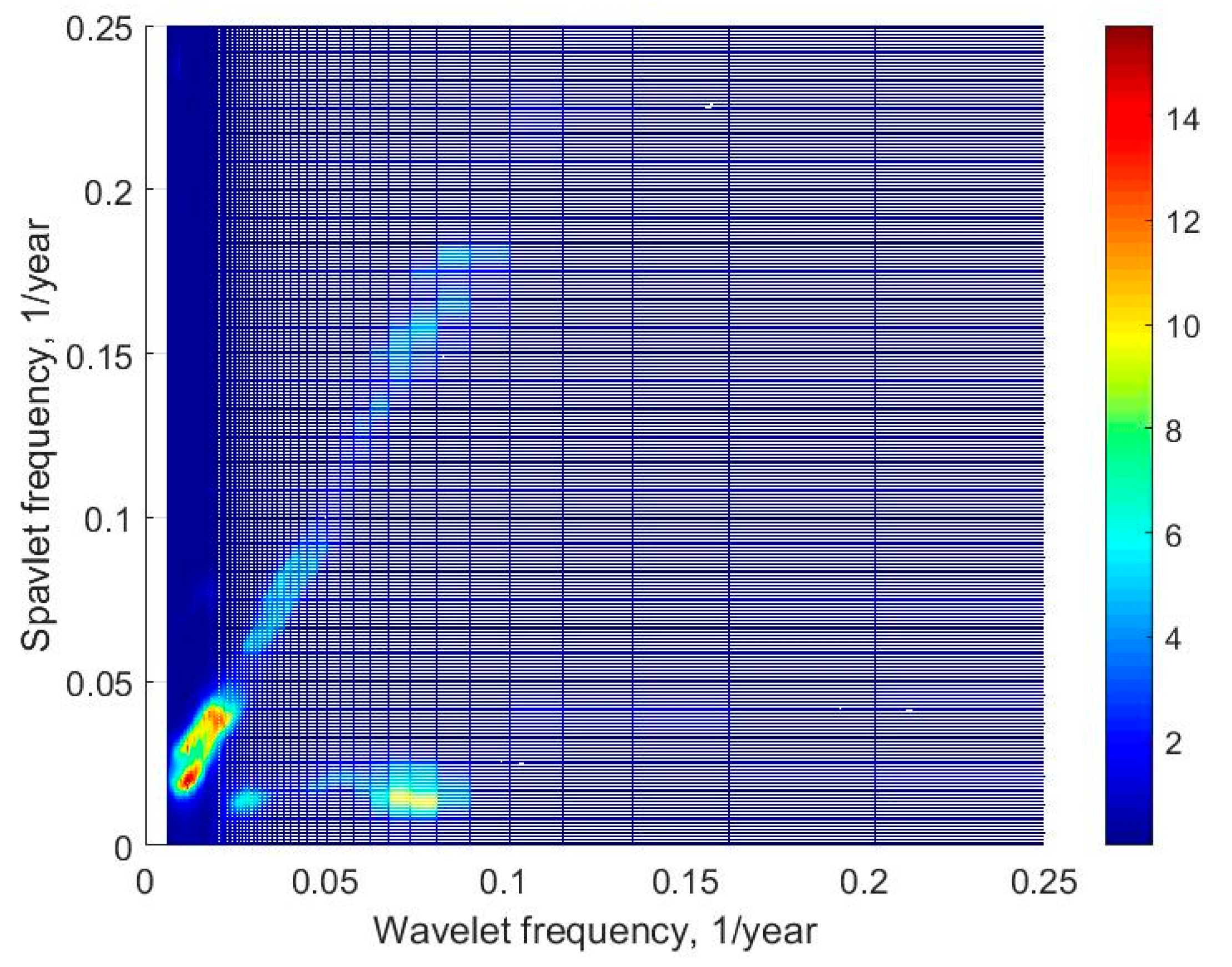
As can be seen from Formula (3), the energy nonlinearly depends on the wave height and linearly on the wave period. A spavlet analysis revealed that the changes of the power flux of wave energy at frequencies 0.03 and 0.075 are modulated by a low frequency of 0.016 year−1 (Figure 9).
From the structure of the spavlets, the fluctuations of power flux of wave energy can be approximately described by a function:
where coefficients A, B, and C should be determined empirically.
FE (t) = A3cos(0.016t) + B3cos(0.016t)cos(0.03t) + C3cos(0.016t)cos(0.075t),
The first term of right part of Equation (5) is similar to Equations (1) and (2). The second term of Equation (5) is determined by the change in the average annual period of waves (Equation (2)), and the third by the change of average annual wave heights (Equation (1)). Note that the frequency 0.016 year−1 is also present in the spavlets of the average annual heights, periods, and of the power flux of wave energy; it is also present in spavlets of all considered climatic indices as the fundamental frequency and as the modulating frequency. It is possible that the fluctuations of this period reflect the trends of global climate change.
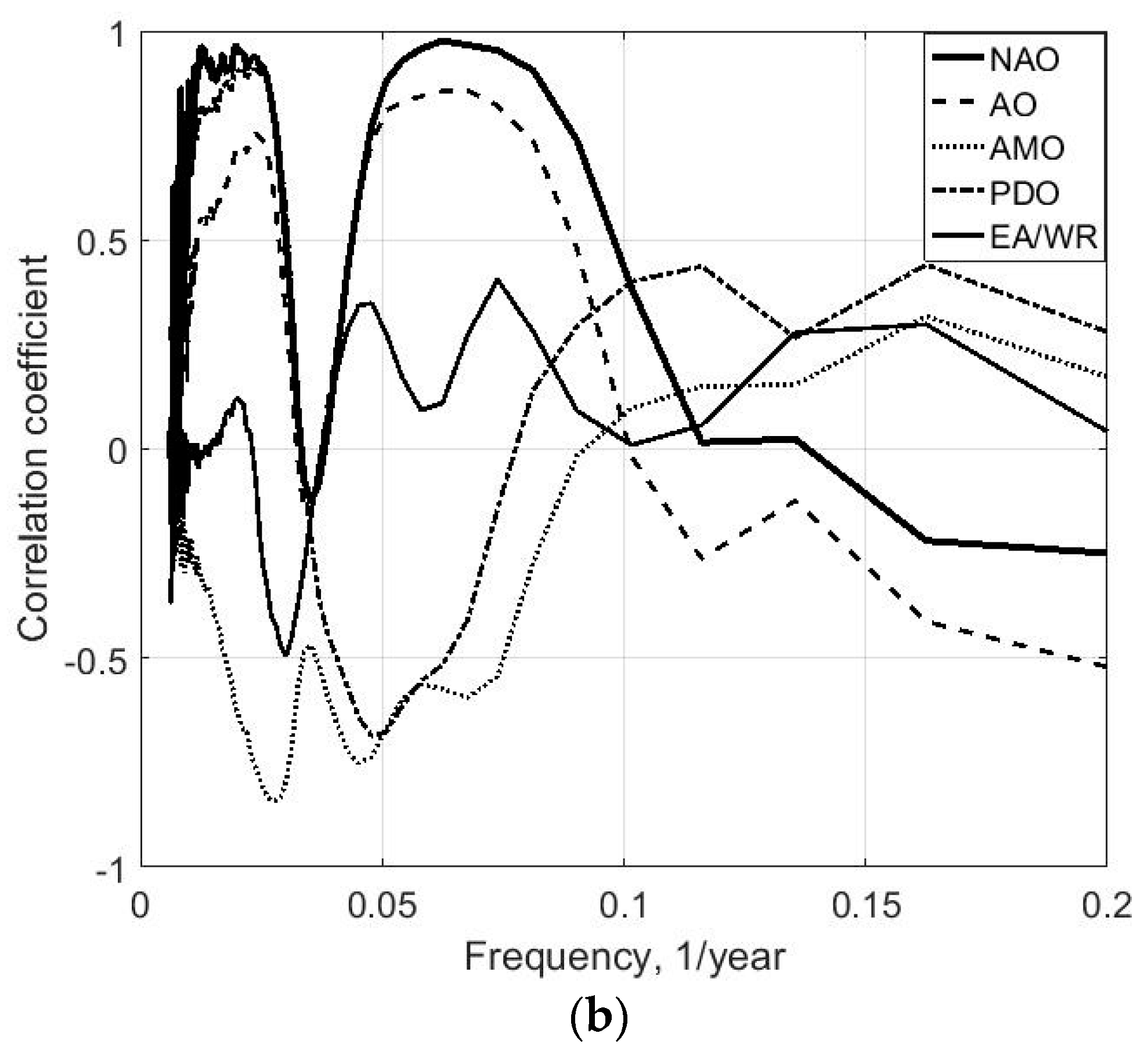
In Figure 10, the coefficients of wavelet-correlation functions between the power flux of wave energy and climatic indices at zero time lags are shown.
Clearly, long–term changes of the power flux for the periods of 50–60 years is associated with the change in EA/WR and AMO climatic indices: for the 40-year period with the indices of PDO, AO and NAO; for the 30–35-year period with EA/WR and AMO indices; for the 20–25-year periods with EA/WR, AO, and PDO indices. In addition, the variability of the NAO index will influence the changes of the power flux of wave energy with a periodicity about 15 years: for the variability of EA/WR index, a periodicity of about 13 years; for the variability of AO index, a periodicity of about 15 and 5 years. Thus, the short-term variability of the power flux of wave energy is associated with changes to NAO, EA/WR, and AO climatic indices.
Thus, the expected decrease in power flux of wave energy for a periodicity of 50–60 years is associated with the positive phase of AMO, whereas a periodicity of 40 years is associated with the positive phase of NAO, PDO, AO, and the negative phase of AMO. The increase in power flux of wave energy will occur in the positive phases of all periods of the EA/WR change with a frequency of 50–60, 20–25, and 13 years, as well as with a periodicity of 15 years in association with the positive phase of the NAO and AO for this period of variability. After a comparison of the changes in climatic indices and wave energy (Figure 4 and Figure 8) and also on the basis of the wavelet correlation analysis, it can be assumed that a significant decrease in power flux of wave energy in the mid-1980s is associated with a positive phase of PDO and NAO for long-term periods, and the largest increase in the early 1990s is associated with a positive phase of short-period changes of NAO, AO, and EA/WR.
5. Conclusions
As a result of an analysis, which used Voluntary Observing Ship Program wave data, it was found that the average power flux of the wave energy in the Black Sea during the period 1960–2011 was 2.43 kW/m, and the highest value was 4.2 kW/m. These values correspond to the estimations made earlier on the basis of modelling data [5,6,7,8,9].
The fluctuations of the power flux of wave energy are connected with changes of the wave climate, which depend on changes in the global climate and are determined by fluctuations of the teleconnection patterns such as the North Atlantic Oscillation (NAO), the Atlantic Multi-decadal Oscillation (AMO), the Pacific Decadal Oscillation (PDO), and the East Atlantic/West Russia (EA/WR). It has been shown that the changes in the average annual wave heights are primarily affected by NAO and, for the average annual wave periods, by PDO.
On the basis of a spavlet analysis, the approximation functions of the changes of the average annual wave heights, periods, and the power flux of wave energy were proposed.
The wavelet-correlations testified to a significant relationship between the changes of the power flux of wave energy and climatic indices, such as NAO, PDO, AO, AMO, and EA/WR. The main long-term periods of the fluctuations are 40, 30–35, and 20–25 years. The short-term periods of the changes of the power flux of wave energy of approximately 13–15 and 5 years are related to oscillations of NAO, EA/WR, and AO climatic indices.
It has been shown that the positive phase of long-term changes in NAO and AO (40 years) leads to a decrease of power flux of wave energy; the positive phase of short-period (15 years) fluctuation of these indices leads to an increase of power flux of energy. The positive phase of changes of the EA/WR for all periods leads to an increase of power flux of wave energy. Concurrently, the decrease of power flux of wave energy correlates well with the positive phase of long-term changes in PDO (40 years) and AMO (50–60 years).
The obtained results show that, in the implementation of any wave energy extraction projects, it is necessary to make an analysis of estimates of the possible energy potential, taking into account long-term climate variability.
Author Contributions
Conceptualization, data analysis, data preparation, main investigation, and writing of paper was done by Y.S.; Spavlet analysis was conducted by S.K.; All authors read, discussed, and approved the manuscript.
Funding
The work was partly supported by the Russian Foundation for Basic Research (grant No. 16-55-76002 ERA_a) in the frame of BS STEMA project.
Acknowledgments
The work was carried out within the framework of state task (theme No. 0149-2018-0015). The authors are grateful to Vika Grigorieva for personal communications and who kindly provided materials about the accuracy of the VOS data.
Conflicts of Interest
The authors declare no conflict of interest.
References
- Rusu, E.; Onea, F. A review of the technologies for wave energy extraction. Clean Energy 2018, 2, 10–19. [Google Scholar] [CrossRef] [Green Version]
- Gunn, K.; Stock-Williams, C. Quantifying the global wave power resource. Renew. Energy 2012, 44, 296–304. [Google Scholar] [CrossRef]
- Atan, R.; Goggins, J.; Nash, S. A detailed assessment of the wave energy resource at the Atlantic Marine Energy Test Site. Energies 2016, 9, 967. [Google Scholar] [CrossRef]
- Guedes Soares, C.; Bento, A.R.; Goncalves, M.; Silva, D.; Martinho, P. Numerical evaluation of the wave energy resource along the Atlantic European coast. Computers Geosci. 2014, 71, 37–49. [Google Scholar] [CrossRef]
- Galabov, V. The Black Sea Wave Energy: The Present State and the Twentieth Century Changes. Available online: https://arxiv.org/pdf/1507.01187.pdf (accessed on 21 May 2018).
- Rusu, L. Assessment of the wave energy in the Black Sea based on a 15-year hindcast with data assimilation. Energies 2015, 8, 10370–10388. [Google Scholar] [CrossRef]
- Divinsky, B.V.; Kosyan, R.D. Spatiotemporal variability of the Black Sea wave climate in the last 37 years. Cont. Shelf Res. 2017, 136, 1–19. [Google Scholar] [CrossRef]
- Akpınar, A.; Kömürcü, M.İ. Wave energy potential along the south-east coasts of the Black Sea. Energy 2012, 42, 289–302. [Google Scholar] [CrossRef]
- Akpınar, A.; Kömürcü, M. Assessment of wave energy resource of the Black Sea based on 15-year numerical hindcast data. Appl. Energy 2012, 101, 502–512. [Google Scholar] [CrossRef]
- Bromirski, P.D.; Cayan, D.R. Wave power variability and trends across the North Atlantic influenced by decadal climate patterns. J. Geophys. Res. Oceans 2015, 120, 3419–3443. [Google Scholar] [CrossRef] [Green Version]
- Vespremeanu-Stroe, A.; Tatui, F. The influence of North Atlantic Oscillation on Romanian Black Sea coast wind regime. Analele Universitatii din Bucuresti Seria Geografie 2005, 64, 17–26. [Google Scholar]
- Polonsky, A.; Evstigneev, V.; Naumova, V.; Voskresenskaya, E. Low-frequency variability of storms in the northern Black Sea and associated processes in the ocean-atmosphere system. Reg. Environ. Change 2014, 14, 1861–1871. [Google Scholar] [CrossRef]
- Zainescu, F.; Tatui, F.; Valchev, N.; Vespremeanu-Stroe, A. Storm climate on the Danube delta coast: evidence of recent storminess change and links with large-scale teleconnection patterns. Nat. Hazards 2017, 87, 599–621. [Google Scholar] [CrossRef]
- Masselink, G.; Austin, M.; Scott, T.; Poate, T.; Russell, P. Role of wave forcing, storms and NAO in outer bar dynamics on a high-energy, micro-tidal beach. Geomorphology 2014, 226, 76–93. [Google Scholar] [CrossRef] [Green Version]
- Saprykina, Y.V.; Kuznetsov, S.Y. Methods of analysis of nonstationary variability of wave climate of Black Sea. Phys. Oceanogr. 2018, 4, 156–164. [Google Scholar]
- Rusu, L.; Bernardino, M.; Guedes Soares, C. Wind and wave modelling in the Black Sea. J. Op. Oceanogr. 2014, 7, 5–20. [Google Scholar] [CrossRef] [Green Version]
- Cherneva, Z.; Guedes Soares, C.; Andreeva, N. Wind and wave climate over the Black Sea. In Maritime Technology and Engineering, 2nd ed.; Guedes Soares, C., Santos, T.A., Eds.; Taylor & Francis Group: London, UK, 2015; pp. 1309–1316. [Google Scholar]
- Shtremel, M.; Saprykina, Y.; Kuznetsov, S.; Ayat Aydoğan, B.; Aydoğan, B. Wave climate of the Black Sea: Visual Observations and Modelling Data. In Proceedings of the 13th International MEDCOAST Congress on Coastal and Marine Sciences, Engineering, Management & Conservation (MEDCOAST 17), Mellieha, Malta, 30 October–4 November 2017. [Google Scholar]
- Aydoğan, B.; Ayat Aydoğan, B.; Yüksel, Y. Black Sea wave energy atlas from 13 years hindcasted wave data. Renew. Energy 2013, 57, 436–447. [Google Scholar] [CrossRef]
- Silva, D.; Rusu, E.; Guedes Soares, C. Evaluation of various technologies for wave energy conversion in the Portuguese nearshore. Energies 2013, 6, 1344–1364. [Google Scholar] [CrossRef]
- World Wide Voluntary Observing Ship Program. Available online: https://www.vos.noaa.gov/ (accessed on 30 July 2018).
- Hogben, N.; Da Cunha, L.F.; Oliver, H.N. Global Wave Statistics; Unwin Brothers Limited: London, UK, 1986. [Google Scholar]
- Soares, C.G. Assessment of the uncertainty in visual observations of wave height. Ocean Eng. 1986, 13, 37–56. [Google Scholar] [CrossRef]
- Vettor, R.; Guedes Soares, C. Rough weather avoidance effect on the wave climate experienced by oceangoing vessels. Appl. Ocean Res. 2016, 59, 606–6015. [Google Scholar] [CrossRef]
- Gulev, S.K.; Grigorieva, V.; Sterl, A.; Woolf, D. Assessment for the reliability of wave observations from voluntary observing ships: insights from the validation of a global wind wave climatology based on voluntary observing ship data. J. Geophys. Res. 2003, 108, 3236. [Google Scholar] [CrossRef]
- Grigorieva, V.; (Shirshov Institute of Oceanology, Moscow, Russia). Personal communication, 2018.
- Grigorieva, V.G.; Gulev, S.K.; Gavrikov, A.V. Global historical archive of wind waves based on voluntary observing ship data. Oceanology 2017, 57, 229–231. [Google Scholar] [CrossRef]
- Grigorieva, V.G.; Badulin, S.I. Wind wave characteristics based on visual Observations and satellite altimetry. Oceanology 2016, 56, 19–24. [Google Scholar] [CrossRef]
- Gulev, S.K.; Grigorieva, V.; Sterl, A. World Ocean Waves (WOW). Available online: http://www.sail.msk.ru/wow/ (accessed on 11 July 2018).
- National Oceanic & Atmospheric Administration. Available online: https://www.esrl.noaa.gov/psd/data/climateindices/list/ (accessed on 30 July 2018).
- Torrence, C.; Compo, G.P. A practical guide to wavelet analysis. Bull. Am. Meteorol. Soc. 1998, 79, 61–78. [Google Scholar] [CrossRef]
- Petenko, I.V. Advanced combination of spectral and wavelet analysis (“spavlet analysis”). Bound.-Layer Meteorol. 2001, 100, 287–299. [Google Scholar] [CrossRef]
Figure 1.
Distribution of observation points for period 1960–2011 along the Black Sea (a), the total number of observations per year (b), and the dependence of the average annual wave height on the number of observations (c).
Figure 1.
Distribution of observation points for period 1960–2011 along the Black Sea (a), the total number of observations per year (b), and the dependence of the average annual wave height on the number of observations (c).

Figure 2.
Changes of average annual wave periods (a) and heights (b), VOS data.

Figure 3.
Wavelet transforms of the average annual wave periods (a) and heights (b). For wavelet analysis, the mean values of the time series were deleted.
Figure 3.
Wavelet transforms of the average annual wave periods (a) and heights (b). For wavelet analysis, the mean values of the time series were deleted.

Figure 4.
Wavelet transforms of NAO (a), AMO (b), AO (c), PDO (d) and EA/WR (e). For wavelet analysis, the mean values of the time series were deleted.
Figure 4.
Wavelet transforms of NAO (a), AMO (b), AO (c), PDO (d) and EA/WR (e). For wavelet analysis, the mean values of the time series were deleted.

Figure 5.
Spavlets of the average annual wave heights (a) and periods (b).


Figure 6.
Spavlets of NAO (a) and PDO (b).


Figure 7.
Coefficients of wavelet-correlation functions between climatic indices and average annual wave periods (a) and heights (b) at zero time lags.
Figure 7.
Coefficients of wavelet-correlation functions between climatic indices and average annual wave periods (a) and heights (b) at zero time lags.


Figure 8.
Change of the power of wave energy flux.

Figure 9.
Spavlet of the power flux of wave energy.

Figure 10.
Coefficients of wavelet-correlation functions between the climatic indices and the power flux of wave energy at zero time lags.
Figure 10.
Coefficients of wavelet-correlation functions between the climatic indices and the power flux of wave energy at zero time lags.


Table 1.
Comparisons of resolution of VOS, altimetry, and buoys data (data provided by Grigorieva).
| Parameter | VOS | Altimetry | Buoys Data |
|---|---|---|---|
| Wave height | 0.5 m | 0.4 m | 0.2 m |
| Wave period | 1 s | – | ≥1 s |
| Wind speed | 1 m/s | 1.5 m/s | 1 m/s |
| Direction | 10° | 17–20° | 10° |
© 2018 by the authors. Licensee MDPI, Basel, Switzerland. This article is an open access article distributed under the terms and conditions of the Creative Commons Attribution (CC BY) license (http://creativecommons.org/licenses/by/4.0/).
Share and Cite
MDPI and ACS Style
Saprykina, Y.; Kuznetsov, S. Analysis of the Variability of Wave Energy Due to Climate Changes on the Example of the Black Sea. Energies 2018, 11, 2020. https://doi.org/10.3390/en11082020
AMA Style
Saprykina Y, Kuznetsov S. Analysis of the Variability of Wave Energy Due to Climate Changes on the Example of the Black Sea. Energies. 2018; 11(8):2020. https://doi.org/10.3390/en11082020
Chicago/Turabian StyleSaprykina, Yana, and Sergey Kuznetsov. 2018. "Analysis of the Variability of Wave Energy Due to Climate Changes on the Example of the Black Sea" Energies 11, no. 8: 2020. https://doi.org/10.3390/en11082020
Note that from the first issue of 2016, this journal uses article numbers instead of page numbers. See further details here.