Spatial Environmental Assessment Tool (SEAT): A Modeling Tool to Evaluate Potential Environmental Risks Associated with Wave Energy Converter Deployments

Abstract

Wave energy converter (WEC) arrays deployed in coastal regions may create physical disturbances, potentially resulting in environmental stresses. Presently, limited information is available on the nature of these physical disturbance or the resultant effects. A quantitative Spatial Environmental Assessment Tool (SEAT) for evaluating the potential effects of wave energy converter (WEC) arrays on nearshore hydrodynamics and sediment transport is presented for the central Oregon coast (USA) through coupled numerical model simulations of an array of WECs. Derived climatological wave conditions were used as inputs to the model to allow for the calculation of risk metrics associated with various hydrodynamic and sediment transport variables such as maximum shear stress, bottom velocity, and change in bed elevation. The risk maps provided simple, quantitative, and spatially-resolved means of evaluating physical changes in the vicinity of a hypothetical WEC array in response to varying wave conditions. The near-field risk of sediment mobility was determined to be moderate in the lee of the densely spaced array, where the potential for increased sediment deposition could result in benthic habitat alteration. Modifications to the nearshore sediment deposition and erosion patterns were observed near headlands and topographic features, which could have implications for littoral sediment transport. The results illustrate the benefits of a risk evaluation tool for facilitating coastal resource management at early market marine renewable energy sites.

1. Introduction

Wave energy has enormous potential for supporting energy security and reducing greenhouse gas emissions. For example, it has been estimated that the recoverable wave resource potential along the United States outer continental shelf is 1170 TWh/year [1]. This amounts to over a quarter of the United States’ total annual electricity consumption. Wave energy converter (WEC) technology development over the past few decades has produced a wide array of wave energy technologies. The International Energy Agency Ocean Energy Systems has developed categories to describe these technologies, which include oscillating water columns, wave activated bodies (floating point absorbers), and overtopping device archetypes [2]. Within these categories, the European Marine Energy Center has counted over 250 developers to date, showing the significant interest in wave energy conversion [3].

Scaled versions of commercial devices are currently being tested in dedicated wave tanks as well as at oceanic test sites [4,5,6]. While present-day testing has generally involved laboratory-scale devices or single devices, arrays of multiple ocean-deployed WEC devices will be necessary for commercial-scale wave energy conversion to onshore electrical power. These WEC arrays, or wave farms, may conflict with other ocean uses, e.g., shipping and navigation, commercial fishing, and recreation [7]. Wave farms consisting of tens to hundreds of devices may have combinations of beneficial and adverse near- and far-field physical effects on the marine environment, such as changes to wave characteristics, circulation patterns, and sediment dynamics (e.g., [8,9,10,11,12,13,14,15]).

Characterization of the physical environment and associated potential alteration of an environment due to a single WEC or arrays of WECs must be ascertained in order to make informed predictions of device performance, system design requirements for hydrodynamic loads, and resource management decisions based on environmental responses. The survivability and maintainability of wave energy devices is directly influenced by nearshore circulation and waves, primarily where WEC infrastructure (e.g., anchors, piles) is exposed to ocean hydrodynamic forces. The WEC-associated infrastructure has the potential to modify the circulation in the water column and, depending on the location, may alter important environmental processes. For example, nutrient delivery, light availability, benthic habitat, larval motility, and many other environmental parameters may be changed by WEC-induced alteration of circulation and sediment transport patterns, thereby affecting marine and shoreline ecosystems [16].

Multiple numerical case studies have quantified the effects of wave farms on coastal processes and assessed the influences of WECs on hydrodynamics and device performance. The optimum wave farm layout for the Wave Dragon WEC was determined by Beels et al. [9] by investigating wake effects using a mild-slope wave propagation model. O’Boyle et al. [17] performed wave tank experiments to evaluate near-field wave disturbances from wave scattering and radiation around different array layouts of five oscillating water column WECs. These studies suggest that the effects of the wave farm layout on hydrodynamics due to wave scattering can be controlled by device spacing relative to wavelengths typical to the wave energy site. They also determined that wave radiation effects were found to be significant and dependent on WEC device performance characteristics and stated the importance of considering these characteristics when optimizing power capture or evaluating WEC effects on nearshore processes. Similar to O’Boyle et al. [17], Özkan-Haller et al. [15] performed wave tank experiments and numerical modeling to investigate wave field modifications in the presence of WECs. Their results suggested that the downstream environmental effects of WEC arrays may be diminished through device operational changes, specifically indicating that WECs should be designed to operate in a wave climate that is equal to or longer than the period of peak energy extraction.

Gonzales-Santamaria et al. [18] discovered significant wave farm impacts on morphological changes at the Wave Hub site (England). The authors quantified littoral transport in the lee of the WEC array and concluded that longshore currents could lead to enhanced deposition in the lee of the wave farm as well as local erosion and a northward shift in erosion and deposition patterns due to wave farm-induced wave diffraction. Abanades et al. [12] used wave and morphodynamic numerical models to investigate the effectiveness of a wave farm as a coastal defense mechanism in Cornwall, England. Their results showed substantial reduction in the erosion of beach profiles and the authors concluded that a wave farm could be considered a viable method of coastal protection. Similarly, Zanopol et al. [19] performed numerical wave and circulation models and ascertained that the northern Romanian coast of the Black Sea may benefit from certain configurations of WEC arrays, which could induce the transport of sediment from the north and enhance shoreline accretion.

Many studies have shown that the deployment of a WEC array has the potential to alter waves and nearshore currents that govern sediment mobility. It is therefore critical to evaluate the potential effects of WEC array deployments and address key physical stressors at a study site, including changes to sediment transport. The primary goal of this study is to describe the Spatial Environmental Assessment Tool (SEAT), a quantitative tool that can be used to provide input to the environmental assessment process by evaluating the potential effects of WECs on waves, circulation, and sediment transport, and thus understand potential environmental risks associated with WEC deployments. The SEAT is not intended to replace the traditional environmental assessment process, but it can provide information on a subset of potential environmental risks. As a baseline example, the SEAT was used to quantitatively assess seabed changes as the result of WEC deployments for a case study off the coast of Newport, Oregon, USA. Two stressors, bottom shear stress and seabed elevation, and metrics specific to each are presented to establish the basis of the SEAT framework for use in evaluating other environmental metrics.

2. Materials and Methods

Nonlinear combinations of winds, tides, and waves typically control nearshore circulation and mixing, with waves being the dominant driver of nearshore circulation in energetic coastlines such as the Oregon coast. Therefore, in order to capture complex wave-, tide-, and wind-induced currents and mixing, the SEAT incorporates a coupled wave, circulation, and sediment transport model with quantitative spatial risk assessment for investigating simulated WECs in nearshore environments. The risk metrics developed for the SEAT relate changes in a stressor (e.g., bottom shear stress) to values considered critical for benthic habitats (e.g., changes in the bottom substrate).

2.1. Study Site

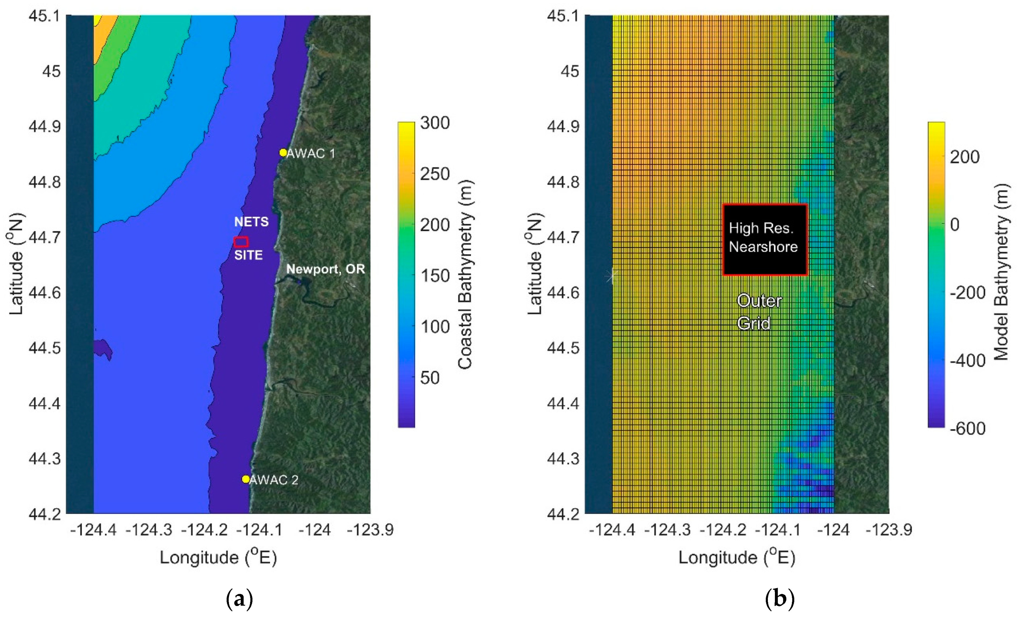
The case study site is located approximately 3.7 km to 5.5 km offshore of Newport, Oregon, USA, north of Yaquina Head, at a water depth of approximately 50 m (Figure 1). The site is known as the North Energy Test Site (NETS) of the Pacific Marine Energy Center (PMEC), where WECs have been deployed and future deployments are planned. This 1.8-km² site was chosen as the potential location of a WEC array due to the available energy resources and limited potential environmental effects. The availability of data necessary for model input boundary conditions, calibration, and validation near NETS is an additional benefit to the evaluation of this site. Long-term wave characterization and current velocity measurements are available through Oregon State University’s (OSU) Acoustic Wave and Current (AWAC; Nortek, Boston, MA, USA) data collected in the summer of 2005 near NETS. Additionally, daily-averaged surface velocities encompassing the model domain are available from two Coastal Ocean Dynamics Applications Radar (CODAR) systems deployed in the area by OSU researchers (http://bragg.oce.orst.edu/ORCoast/).

The waters off Newport, Oregon are characterized by a year-round energetic wave field. Swell heights range from zero to 7 m, swell directions vary seasonally from 180° to 315°, and wave periods range from 4 s to 20 s. The site coastline is defined by pocket beaches up to 16 km long with headlands of large cliffs. Sandy sediment ranging from 100 μm to 500 μm in diameter (fine to coarse sand) compose much of the beach material along the site’s coastline [20,21] and extend into the offshore region [22]. Seasonal variations in storm intensity move sediment between the offshore and nearshore zones. Variations in sediment transport are primarily driven by waves whose bulk statistics vary with the seasons. Winter storms are predominantly from the south. Southerly waves transport sands northward along the beaches where headlands trap sediment and promote deposition [23]. Less energetic summer swells move sediment to the south. Over long periods, this process results in little net sediment transport out of the system due to alongshore transport.

2.2. Spatial Environmental Assessment Tool (SEAT) Coupled Numerical Model

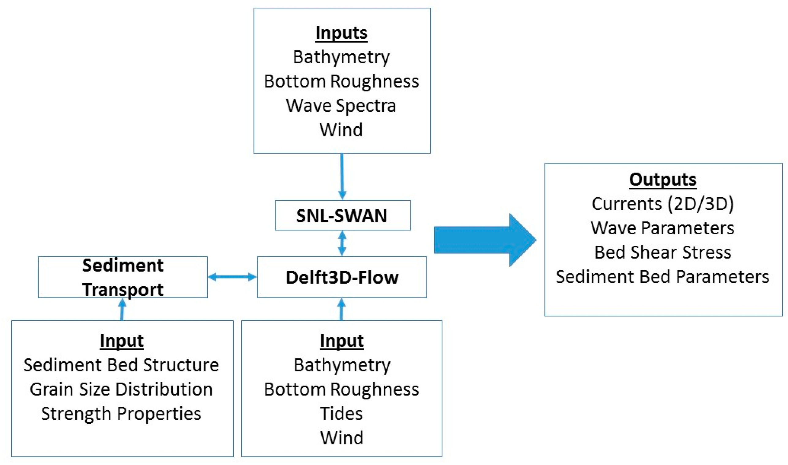
A coupled wave, circulation, and sediment transport model was developed using a hybrid modeling framework (Figure 2). Waves were modeled using a modified version of Simulating WAves Nearshore (SWAN) [24,25], named SNL-SWAN (Sandia National Laboratories-SWAN), which is a module developed by SNL and incorporated into the open-source Delft3D framework. SNL-SWAN incorporates a WEC module that accounts for device-specific WEC power take-off characteristics to more accurately evaluate each device’s effects on wave propagation and ultimately nearshore hydrodynamics [26,27,28,29]. Delft3D-FLOW is a multidimensional hydrodynamic and sediment transport model that is capable of quantifying circulation (non-steady), waves, and sediment transport phenomena as a result of forcing by tides and meteorological processes [30,31]. The coupled model allows for the evaluation of tidal- and wave-driven circulation and sediment transport in the model domain. Within the model framework, WECs are treated as obstacles that allow wave energy to be propagated and to be absorbed by the WECs.

The Newport, Oregon case study model configuration consisted of a three-dimensional (latitude, longitude, depth) nested grid over which circulation and waves were modeled (Figure 2). In Delft3D-FLOW, circulation in a nested grid was modeled as a two-way coupling between grids, while the coupled wave module was run as one-way nesting, meaning information only passed from the outer to the inner grid. The coupled Delft3D-FLOW-SNL-SWAN model simulated the hydrodynamics of tidal- and wave-driven circulation at a 3-s time step for model stability, then coupled the circulation to SNL-SWAN every 3 h to capture variations in the temporal wave field (Figure 2). This two-way coupling of waves and currents allowed for the model to capture the non-linear interactions between currents and waves and the subsequent effects on the system (Case study model set-up files are available in Supplementary Materials).

2.2.1. Model Inputs

Wave propagation and circulation in the coastal zone are fundamentally controlled by bathymetry; therefore, the coupled numerical model required accurate bottom bathymetry data as input. For the Newport, Oregon case study, model depths were defined from the National Oceanic and Atmospheric Administration (NOAA) National Geophysical Data Center high-resolution (approximately 10 m) digital elevation model of the Oregon coast. The bathymetry data was mapped to the model grid using bi-linear interpolation (Figure 1). Generally, the digital elevation model has higher spatial resolution than the computational model. Water depths within the model domain varied from less than 5 m nearshore to over 200 m in the northwestern corner of the computational grid.

2.2.1.1. Circulation Model

Surface currents in the model domain were driven by the application of time varying, spatially uniform winds. Hourly winds were derived from measurements by NOAA National Data Buoy Center (NDBC) buoy station 46089 at the outer edge of the largest-scale model domain (Figure 1). Tidal boundary conditions were applied using the TOPEX/POSEIDON global tide model (TPXO09) interpolated onto the model grid [32]. Water density was assumed constant at 1025 kg/m³ and horizontal eddy viscosity was held constant at 1.0 m²/s throughout the computational domain. Variations in density due to temperature and salinity gradients were not included in these screening level coastal models, but can be readily incorporated into future studies.

2.2.1.2. Wave Model

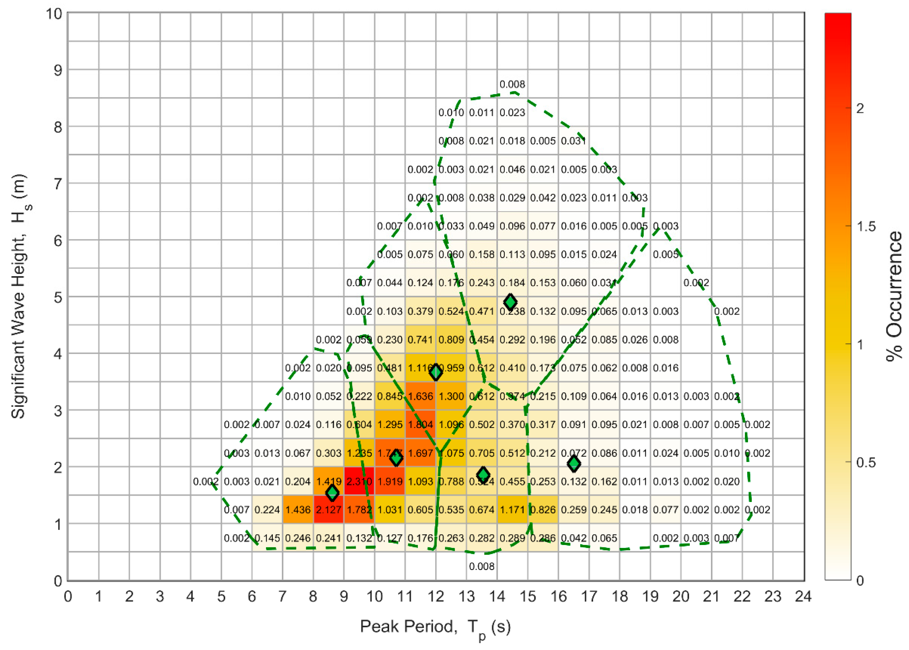
A comprehensive analysis of expected wave conditions on the Oregon coast was conducted using seven years (2005–2011) of modeled wave conditions [33]. This analysis provided approximately 300 discrete sea state bins, characterized by significant wave height (H_s), peak period (T_p), and mean wave direction (D_p) [34], along with the probability of occurrence of each sea state. In order to incorporate directionality into the characterization of the sea states, the data were split into four directional bins (200°–230°, 230°–260°, 260°–290°, 290°–320°) over which the analyzed wave directions were distributed. A joint probability distribution (JPD) of H_s and T_p was calculated for each of the four directional bins (Figure 3).

Clustering analysis (k-means) was used to reduce the number of sea states from 300 events to 24 events for model input following Bull and Dallman [35] (

Table 1. Operational sea states selected for each of the four direction vectors. The sea states are the cluster centers, identified using k-means clustering [35].

Directional Bin	Hs (m)	Tp (s)	Dp (deg)	% of Direction Bin	Total % Occurrence of the Cluster
200°–230°	1.76	6.60	221.8	15.41	0.39
	2.67	8.62	220.8	40.68	1.03
	4.06	10.16	221.3	23.47	0.59
	1.37	15.33	224.0	8.06	0.20
	7.05	12.60	223.6	3.42	0.09
	2.11	11.63	223.8	8.96	0.23
230°–260°	4.91	13.62	251.2	11.99	1.76
	1.70	7.73	244.8	15.03	2.21
	2.69	9.80	247.6	26.75	3.94
	1.23	14.62	248.8	18.54	2.73
	2.31	17.54	249.4	3.97	0.58
	2.94	11.77	250.6	23.72	3.49
260°–290°	4.90	14.43	275.8	8.78	4.70
	1.54	8.62	278.0	20.90	11.19
	3.66	12.00	277.2	20.95	11.21
	2.16	10.71	277.5	25.39	13.59
	1.85	13.54	277.2	16.21	8.67
	2.05	16.51	276.4	7.77	4.159
290°–320°	1.81	9.11	298.6	28.46	8.297
	2.16	13.35	295.7	10.70	3.120
	1.49	7.12	304.6	22.86	6.664
	2.66	11.02	297.2	26.48	7.720
	2.08	16.53	295.6	5.28	1.540
	4.65	13.23	296.2	6.22	1.813

). Briefly, k-means clustering analysis determined the sea states, or cluster centroids, via the minimization of the squared Euclidian distance between each point and a cluster centroid. The number of clusters within each directional bin was defined to be six, and an iterative partitioning method optimized the centroid of each cluster and the cluster size by minimizing the sum of point-to-centroid distances, summed over all six clusters. The resulting sea states generated by k-means are represented by the green diamonds in Figure 3.

The probability of occurrence of each sea state within each direction bin was defined as the number of individual (H_s, T_p) points assigned to a cluster, divided by the total number of (H_s, T_p) data points within a direction sector. Similarly, the probability of occurrence over all direction bins was calculated by dividing by the total number of (H_s, T_p) data points within the entire model data record. The direction, D_p, assigned to the sea states in Table 1 was determined by taking the average of the individual D_p values over the cluster. This process provided a reproducible and adjustable method to characterize the occurrence of site conditions. Clustering analysis enabled the modeling of discrete events based on probability analysis and the development of risk potential based on modeling results. This approach has the benefit of reducing run times by modeling discrete events rather than simulating long-term time series, but becomes limited by the lack of continuity between events. Despite this limitation, pairing the probability of an event with results from the modeled conditions can be used to inform stakeholders of potential long-term effects of a WEC array on a specific environment and vice versa.

The results of clustering analysis provided 24 discrete wave model inputs, characterized by bulk wave parameters (H_s, T_p, and D_p), for the Newport, Oregon case study. Significant wave height ranged from 1.23 m to 7.05 m, peak period ranged from 6.6 s to 17.5 s, and the directional window ranged from 220° to 305° (Table 1). Uniform wave boundary conditions with a JONSWAP spectrum centered on the 24 sets of bulk wave parameters were applied to the SNL-SWAN wave model. While the use of bulk parameter wave conditions (converted to a JONSWAP spectrum) seemingly represents a lower resolution wave model compared to the full spectral specification of boundary conditions, it avoids the contamination of model results by wave conditions that fall outside the pertinent events determined though the cluster analysis described above and will generally represent the peak wave-associated stressors being evaluated.

2.2.1.3. Sediment Transport Module

The Delft3D-FLOW-SNL-SWAN sediment transport module uses vertical layers in the sediment bed to define sediment characteristics and the initial thickness of each initial bed layer defines the amount of sediment available for transport [36]. Sediment layers are defined as fractions of cohesive and noncohesive sediment types, with size classes of various fractions defined in terms of mean diameter (noncohesive) and settling velocity (cohesive sediment). A unique critical shear stress for erosion is associated with each sediment type, and the critical shear stress of the sediment layer is calculated as the weighted fraction of critical shear stresses associated with each size class. Removal of non-cohesive sediment from a parent bed layer (i.e., erosion) occurs if the modeled shear stress exceeds the critical shear stress. Sediment can be advected as a suspended load or a bedload, with the only difference relating to the treatment of transport properties within the water column versus the sediment bed. Erosion rates of the sediment bed for sandy non-cohesive sediment in Delft3D-FLOW-SNL-SWAN are based on empirically defined values [37].

Based on the Coastal and Marine Ecological Classification Standard (CMECS, [22]), the majority of the coastal region within the Newport, Oregon study site is comprised of sandy sediment. However, fine cohesive sediment does exist in the Oregon coastal environment; therefore, three non-cohesive sediment size classes (sands) and one cohesive size class (silt) were incorporated into the calibrated and validated Delft3D-FLOW-SNL-SWAN wave and circulation model. The sandy sediment was represented with grain sizes of 250 μm, 200 μm, and 100 μm in equal fractions and a specific bulk density of 2650 kg/m³, representative of quartz sand. The three grain size classes highlighted differing behaviors of sediment in the environment. Non-cohesive sediment such as mud was included with a settling velocity of 2.5 × 10⁻⁴ m/s.

2.2.2. Model Validation

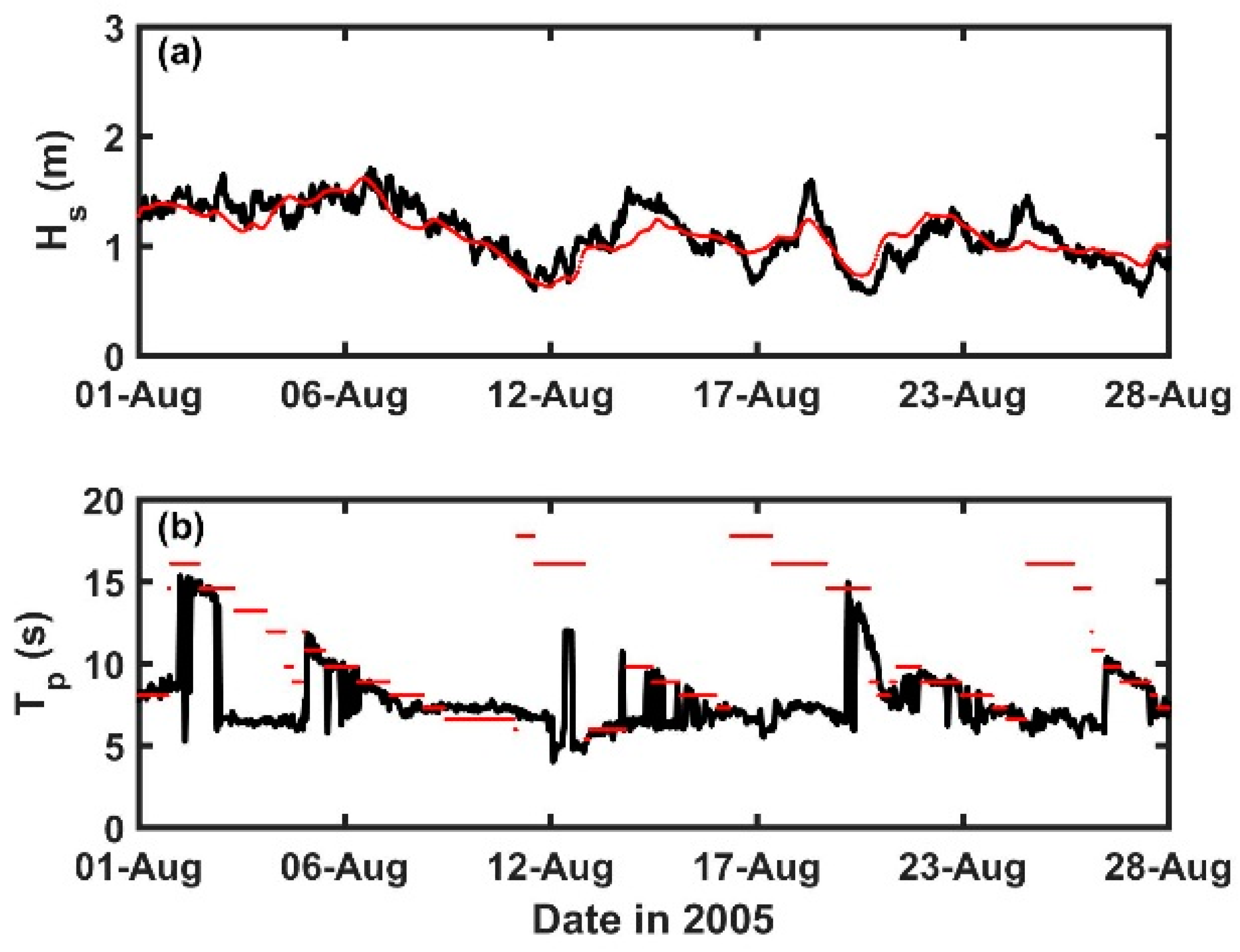
Prior to the introduction of simulated WECs to the coupled numerical model, it was necessary to validate the Delft3D-FLOW-SNL-SWAN model. The model wave and current validation data were provided by in situ CODAR and AWAC measurements within the model domain, collected by OSU researchers. Due to disparate time periods of wave and current data availability, multiple model runs over different time periods were used to compare the flow and wave model results to measurements. The SNL-SWAN wave model was initiated with offshore NOAA NDBC data and validated with in situ directional wave spectra collected by an AWAC deployed at a nearshore location within the model grid (−124.058, 44.8514; AWAC1; Figure 1) at a water depth of 12 m. Modeled versus measured comparisons were made over a 28-day period from 1 to 28 August 2005 during a period of multiple swell conditions, which provided an excellent comparison period for the model (Figure 4). CODAR daily-averaged surface current velocity measurements during a four-week period between 1 and 28 October 2009 were used to validate the circulation model (not shown). Two measurement locations, C1 and C2, were chosen for model validation due to their proximity to the NETS site (Figure 1).

Statistical metrics were determined for modeled versus measured wave parameters and current velocities over the time periods of model validation (see Section 2.2.2) (

Table 2. Comparison of modeled versus measured H_s and T_p and east-west (u) and north-south (v) current velocities. In situ wave data were measured at location AWAC1 (Figure 1). Coastal Ocean Dynamics Applications Radar (CODAR) data were compared for locations south (C1) and west (C2) of the wave energy converter (WEC) array (Figure 1). See Equations (1)–(4) for definitions of Skill, root mean square error (RMSE), Bias, Avg % diff, and Correlation.

Metric	Hs	Tp	u (C1, C2)	v (C1, C2)
Skill	0.90 m	0.90 s	0.7, 0.7 cm/s	0.90, 0.9 cm/s
RMSE	0.18 m	1.90 s	5.6, 6 cm/s	5.5, 6.3 cm/s
Bias	0.09 m	−0.71 s	3.5, 4.1 cm/s	−0.8, 1.4 cm/s
Avg % diff	12.42%	15.51%	18.9%, 13.9%	9%, 7%
Correlation	0.84	0.71	0.8, 0.8	0.9, 0.8

). The metrics included model skill (skill), root mean square error (RMSE), bias, and mean percent difference (Avg % diff), and were computed as follows:

$$\mathrm{Skill}=1-\frac{\sum {\left|\mathrm{modeled}-\mathrm{measured}\right|}^2}{{\left(\sum \left|\mathrm{modeled}-\overline{\mathrm{measured}}\right|+\left|\mathrm{measured}-\overline{\mathrm{modeled}}\right|\right)}^2},$$

(1)

$$\mathrm{RMSE}=\sqrt{\overline{{\left(\mathrm{modeled}-\mathrm{measured}\right)}^2}},$$

(2)

$$\mathrm{Bias}=\mathrm{modeled}-\mathrm{measured},$$

(3)

$$\mathrm{Avg}\%\mathrm{diff}=\overline{100\times \left(\mathrm{modeled}-\mathrm{measured}\right)/\mathrm{measured}},$$

(4)

where overbars indicate means and summation is over the entire model domain. Coefficients of determination (correlation) were determined through least-squares linear regression analysis between modeled and measured quantities. The results demonstrate the excellent ability of the numerical model to reproduce measurements (Table 2; Figure 4).

2.2.3. Case Study Model Runs

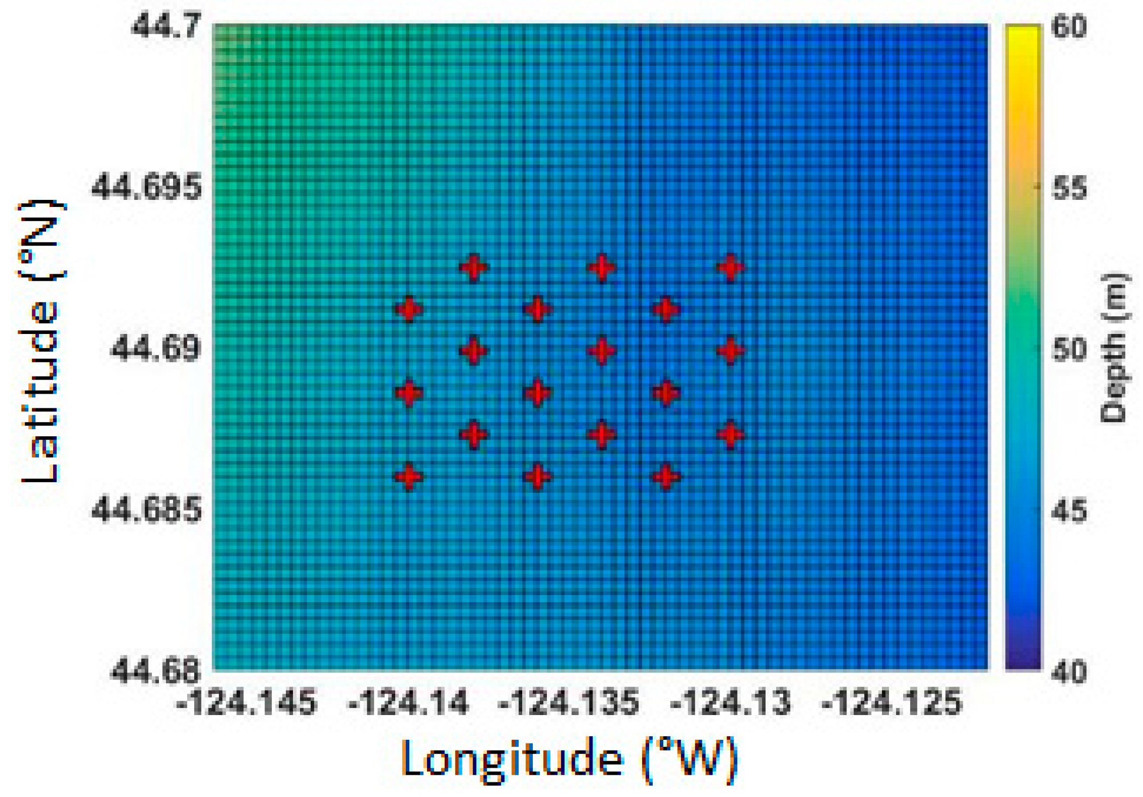
Model runs for the Newport, Oregon case study were conducted for baseline scenarios (no WECs) and WEC scenarios to study the changes within the system due to the presence of WECs. A single type of WEC device was considered for this study, the floating oscillating water column (F-OWC) inspired by the Ocean Energy (OE) Buoy developed by Ocean Energy Ltd., which has a modeled power matrix computed according to Babarit et al. [38] (device characteristics described by Babarit et al. [38]). The power matrix represents the energy extracted from the environment by the device, given a specific sea state prescribed by the significant wave height and peak period. One 18-device array configuration was evaluated at the Newport, Oregon NETS case study site, where each of the 18 modeled devices had a diameter of 50 m spaced 200 m (four diameters) apart in both the east–west and north–south directions (Figure 5).

The fully coupled Delft3D-FLOW-SNL-SWAN model was run for each of the 24 discrete wave events as returned by the cluster analysis (Table 1) with and without a simulated WEC array for a total of 48 model runs. Each model run was conducted for a period of 24 h (approximately two tidal cycles), allowing for variability in tidal conditions to affect sediment transport. Results were compiled at the end of the 24-h period, allowing for 12 h over which sediment could potentially be mobilized. The spin-up period of 12 h allowed the flow model to equilibrate and reduce the potential for numerical instabilities to cause spurious and unwanted changes to the sediment bed. The sediment transport module was run to update the bed thickness with every model time step to simulate the two-way feedbacks between the changing water depth, flow, and wave field and erosion and deposition processes. Following each 24-h model run, the sediment bed at the last time step was chosen for further evaluation. Parameters of interest such as bottom shear stress and bed elevation were extracted at the end of the model run period, and risk metrics were computed.

2.3. SEAT: Risk Assessment

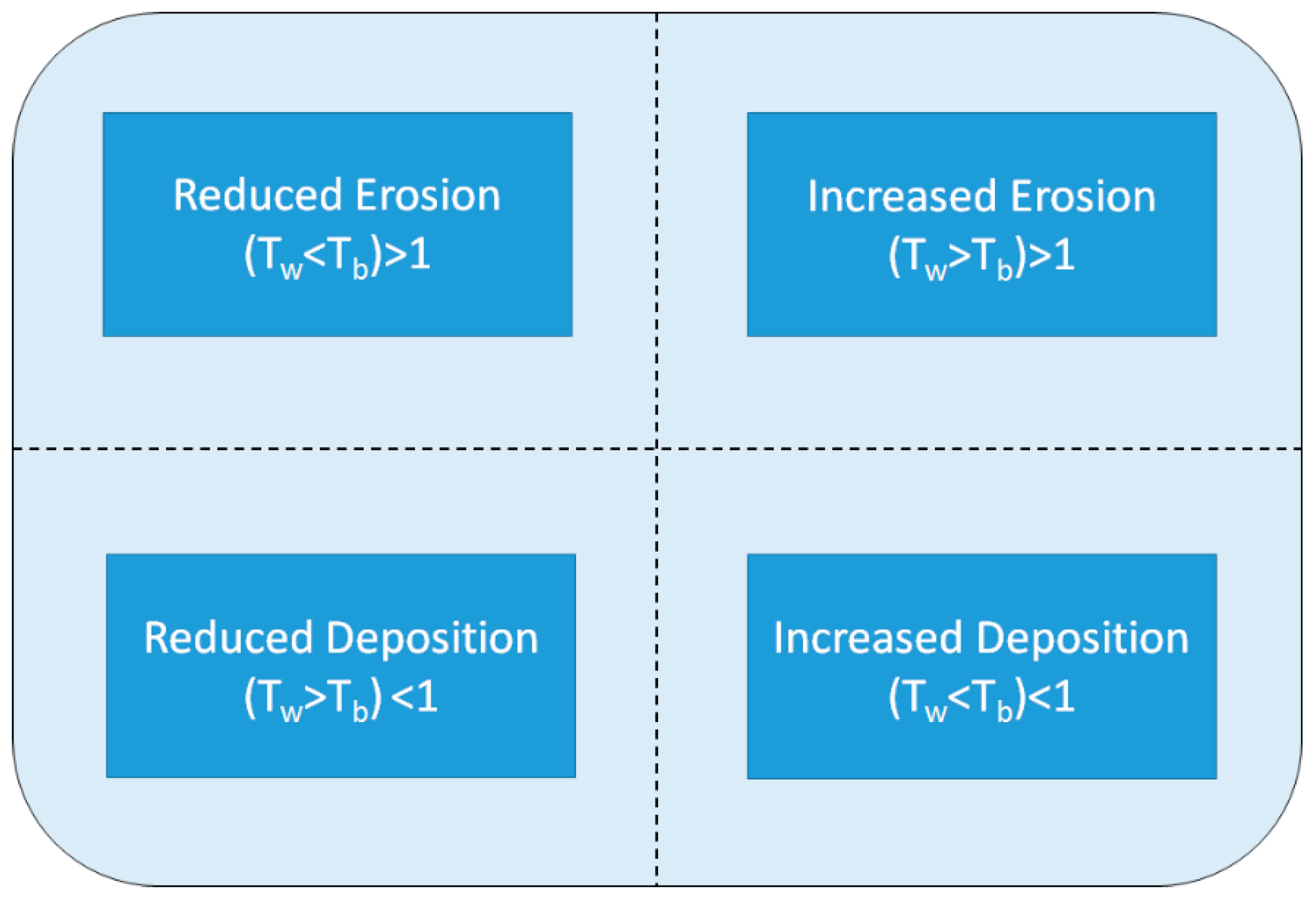
The Newport, Oregon case study focused on two SEAT stressors (near-bed shear stress and seabed elevation) that are considered critical for benthic habitat assessment. The ratio of the shear stress to critical shear stress plays a key role in assessing the risk of sediment mobility associated with the introduction of WECs in an environment. For example, WECs may have the effect of lowering shear stress in the lee of the WEC array. Should the WEC-induced decrease in shear stress result in shear stresses below critical that were once greater than critical prior to the WEC deployment, then an erosional environment would be transformed into a depositional environment. The SEAT therefore defines a sediment transport parameter, T, for each model grid point as:

$$\mathrm{T}\left(\mathrm{x},\mathrm{y}\right)=\frac{\mathsf{\tau }\left(\mathrm{x},\mathrm{y}\right)}{{\mathsf{\tau }}_{\mathrm{c}}\left(\mathrm{x},\mathrm{y}\right)},$$

(5)

where τ and τ_c represent near-bed shear stress and sediment bed critical shear stress and (x,y) denotes model grid points in the longitudinal and latitudinal directions. The sediment transport parameter provides an indication of the ability of sediment to be mobilized. For example, a value of T(x,y) > 1 occurs when shear stresses exceed the critical shear stress of the underlying sediment, as determined by the median particle size of underlying sediment, allowing sediment to be mobilized.

When summed over the 24 cases of wave conditions as returned from the cluster analysis (see Table 1) and dropping the explicit dependence on (x,y), the resulting transport parameter for the baseline (no WECs) scenarios can be expressed as:

$${\mathrm{T}}_{\mathrm{b}}={{\displaystyle \sum }}_{\mathrm{i}}{\mathrm{P}}_{\mathrm{i}}\frac{\mathsf{\tau }}{{\mathsf{\tau }}_{\mathrm{c}}},$$

(6)

where T_b represents the baseline transport parameter and P_i is the probability of the occurrence of the wave event. Similarly, a transport parameter, T_w, was defined for the model scenario with WECs present using the analog of Equation (6). Possible scenarios associated with sediment mobility, based on the relationship between T_b and T_w, and the critical shear stress of the underlying sediment are shown in Figure 6.

Mathematically, the risk of sediment mobility, R_τ, can be defined in terms of a non-dimensional number:

$${\mathrm{R}}_{\mathsf{\tau }}=\mathrm{int}\left(\frac{{\mathrm{T}}_{\mathrm{w}}-{\mathrm{T}}_{\mathrm{b}}}{\left|{\mathrm{T}}_{\mathrm{w}}-{\mathrm{T}}_{\mathrm{b}}\right|}{\mathrm{T}}_{\mathrm{w}}\right)+\left[{\mathrm{T}}_{\mathrm{w}}-{\mathrm{T}}_{\mathrm{b}}\right],$$

(7)

where the int( ) operation represents the integer value of the term. The first term in Equation (7) can be thought of as constraining the risk to the correct quadrant (R < –1, –1 ≤ R < 0, 0 ≤ R < 1, R > 1; see Figure 6). The second term quantifies the risk value within the quadrant. The resulting risk metrics for sediment mobility, Equation (7), therefore consists of four regimes. The first, R_τ ≤ –1, represents a reduction in erosion. The second, –1 < R_τ ≤ 0, represents an increase in deposition. The third, 0 ≤ R_τ < 1, represents a reduction in deposition, and the fourth, R_τ ≥ 1 represents an increase in erosion.

Bottom critical shear stress (and therefore erosion and deposition) is closely related to water depth through the dependences between depth and water column velocities. Physical processes such as tides, waves, and sediment transport result in a change in effective seabed elevation relative to that of a quiescent ocean. The presence of WECs can influence variability in seabed elevation and affect benthic habitats. Therefore, seabed elevation changes were incorporated into the case study risk framework associated with the SEAT. The risk associated with seabed elevation changes associated with WEC deployments was defined as:

$${\mathrm{R}}_{\mathsf{\eta }}={{\displaystyle \sum }}_{\mathrm{i}}{\mathrm{P}}_{\mathrm{i}}\left({\mathsf{\eta }}_{\mathrm{w}}-{\mathsf{\eta }}_{\mathrm{b}}\right)$$

(8)

where η_w and η_b are the seabed elevations in the absence and presence of WECs at each model grid point. Here, R_η has units of elevation (meters) unlike the non-dimensional risk metrics for sediment mobility (Equations (7) and (8)). This difference is primarily due to the difficulty in defining a critical depth of importance to benthic habitat. For example, one could define a critical depth below which eelgrass cannot grow. However, the growth of eelgrass is governed not only by depth, but also by other parameters such as water clarity and photosynthetically available radiation, water column nutrient concentrations, ambient currents, and a host of other environmental parameters. However, in the event that a critical depth for eelgrass growth can be determined for a site, a revised metric similar to Equation (7) can be defined for seabed elevation changes.

3. Results and Discussion

3.1. Wave Energy Converter (WEC) Effects on Sediment Transport

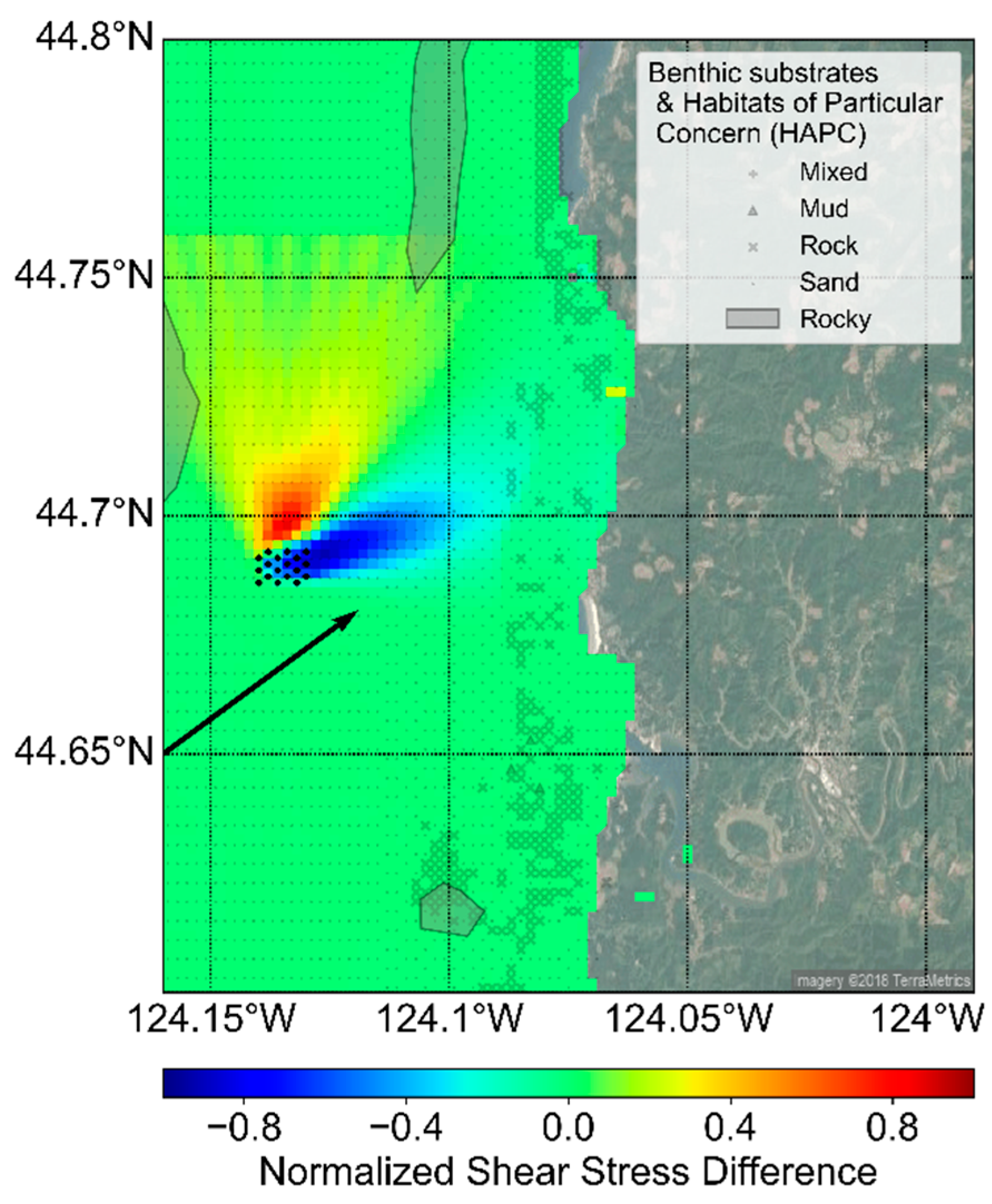
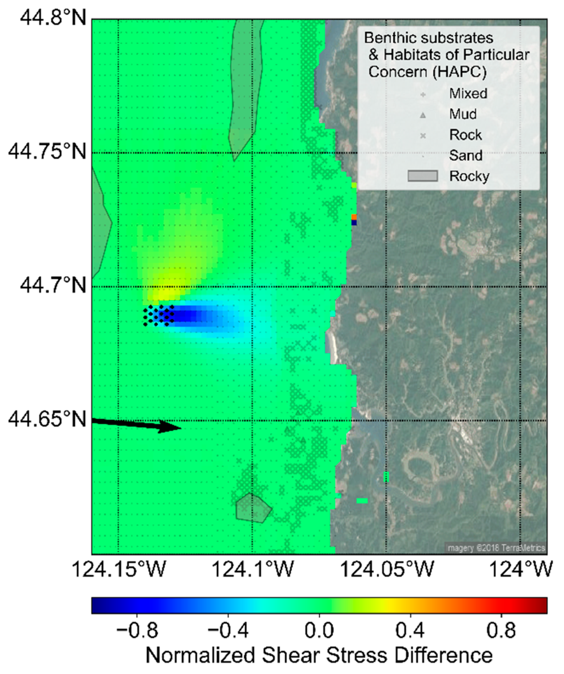
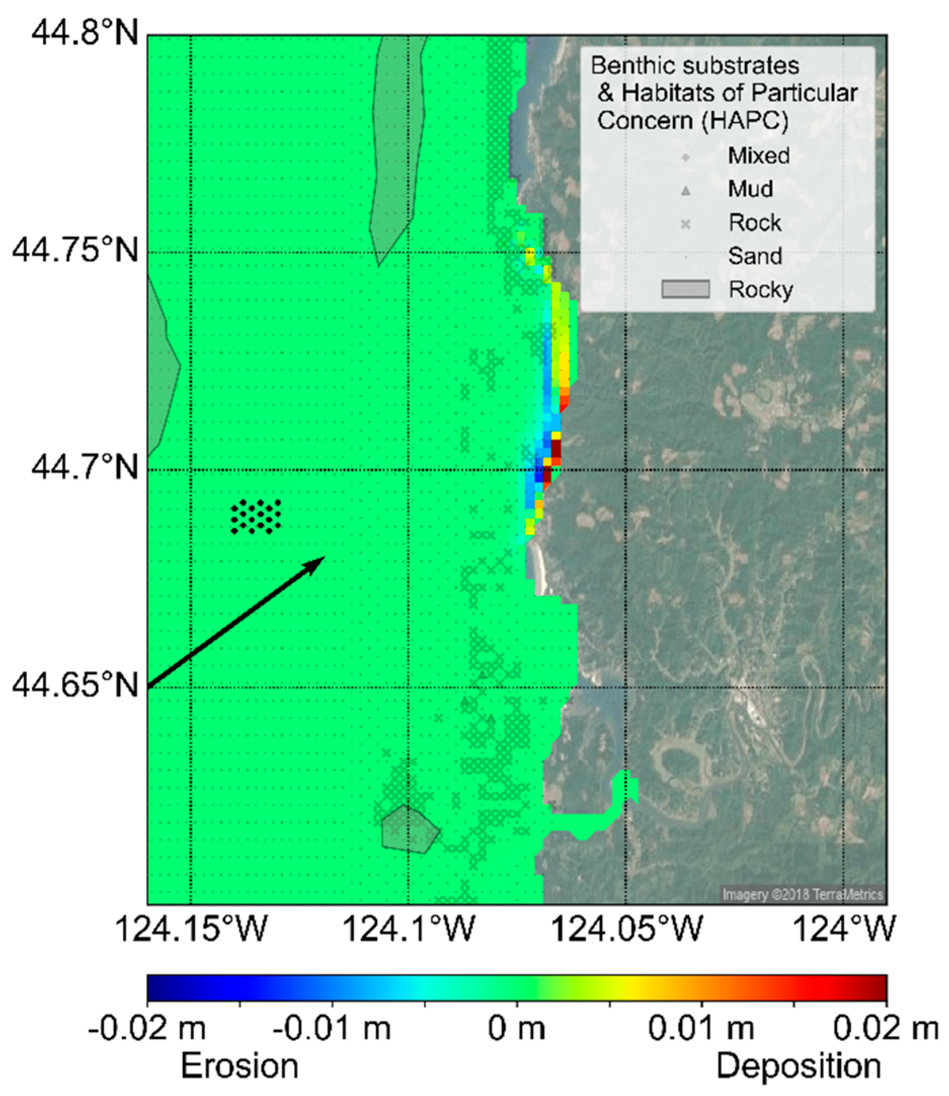
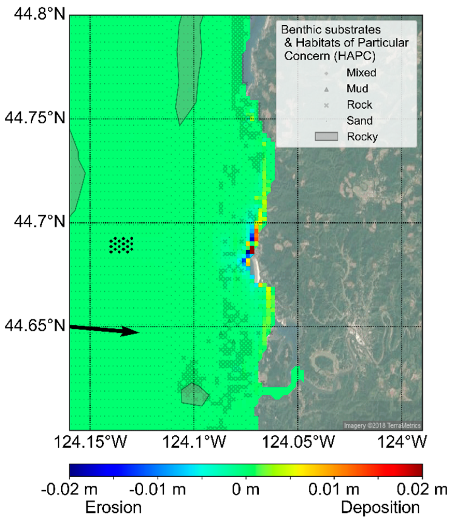
The fully coupled Delft3D-FLOW-SNL-SWAN model of the SEAT framework enables the assessment of changes in hydrodynamic and sediment transport parameters simulated with and without WECs in the environment. For the Newport, Oregon case study, maximum shear stress and bed elevation change were identified as two key parameters that influence variability in nearshore morphological characteristics. Two wave events with the highest annual probability of occurrence out of a total of 24 events were simulated within the SEAT framework and normalized changes in shear stress and change in bed elevation with and without an array of WECs for these two wave events were evaluated (Figure 7, Figure 8, Figure 9 and Figure 10), where normalized change = $\frac{{\mathrm{N}}_{\mathrm{W}}-{\mathrm{N}}_{\mathrm{b}}}{\left|{\mathrm{N}}_{\mathrm{b}}\right|}$ and change = ${\mathrm{N}}_{\mathrm{W}}-{\mathrm{N}}_{\mathrm{b}}$. The parameters N_W and N_b represent shear stress or bed elevation in the presence and absence of WECs, respectively. Therefore, negative values of normalized change indicate decreases in values as the result of the WEC array and vice versa. The two wave events shown are typical of summer (Figure 7 and Figure 9) and winter (Figure 8 and Figure 10) conditions on the Oregon coast.

The SEAT numerical model results indicate that variations in normalized shear stress are primarily observed in the vicinity of the WECs. During conditions typical of summer and winter, decreases in shear stress are observed to occur at the WECs and in the lee of the WEC array along an approximately 15-km swath oriented in the same direction as peak wave direction. Shear stress increased to the north of the WEC array in both cases in the presence of WECs. In winter conditions, reductions in normalized shear stress exceeded increases to the north of the array. It is important to note that while there are noticeable changes in normalized shear stress in the vicinity of the WEC array, absolute changes in shear stress are generally insufficient to cause significant changes in coastal sediment transport as the magnitudes are much lower than the critical shear stress for sediment mobility; however, even small changes can have implications on the nearshore circulation where sediment is mobile. For example, if shear stresses are above the critical shear stress for erosion in the absence of WECs, then the reduction in velocity in the lee of the WEC can change an erosional environment to a depositional environment.

Wave shadowing and coastal transport processes resulted in changes in modeled bed elevation between the presence and absence of WECs, which were expected [20]. While minimal, the wave shadow in the lee of the WEC array, in simulations in the presence of WECs, resulted in enhanced deposition in the nearshore regions (<20 m water depth). A corresponding reduction of deposition was observed in adjacent offshore cells. These deviations were in the order of 0.5% relative to the simulations in the absence of WECs. Interestingly, greater changes in the nearshore sediment bed were observed during summer as compared to winter conditions. It is likely that this is due to a combination of Yaquina Head acting as a wave shadow for the peak wave direction of 224° during summer conditions as compared to 277° during winter and the shift in the peak wave period from 15 s (summer) to 10 s (winter), (Figure 9 and Figure 10).

3.2. SEAT Risk Analysis

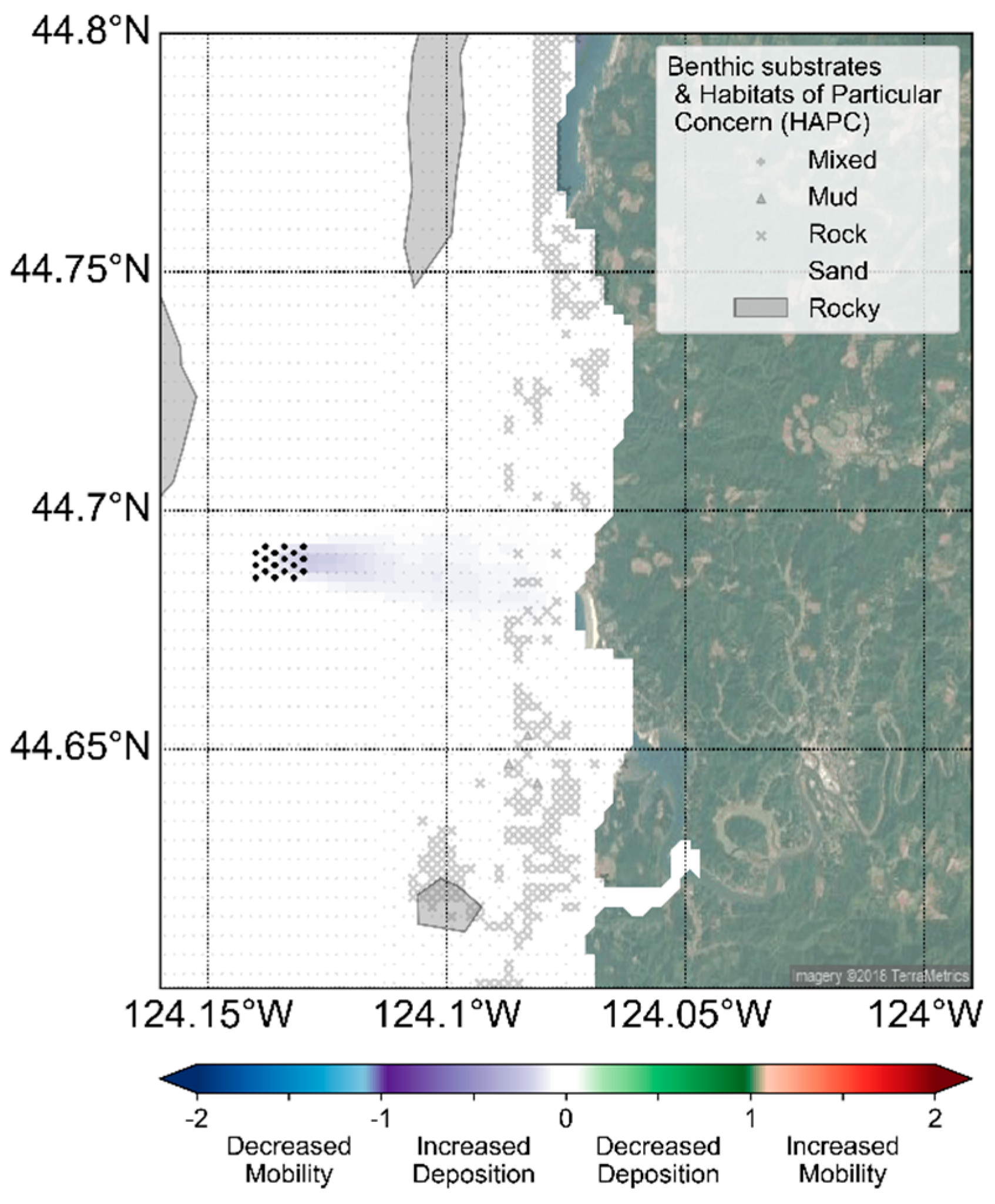
The SEAT enables the application of the probabilistic framework to compute the risk associated with key potential stressors to the marine environment. Figure 11 shows the risk of sediment mobility (R_τ) (Equation (7)) for the Newport, Oregon case study in the context of habitats of particular concern (HAPC), as defined by CMECS [22]. As can be expected, there are moderate changes to sediment mobility in the lee of a WEC array, with expected increased deposition. However, all of these changes are in a region where the potential for changes in deposition rates are naturally limited by sediment supply and are therefore not significant. Most importantly, little to no risk is seen in HAPC, such as rocky reefs and kelp patches.

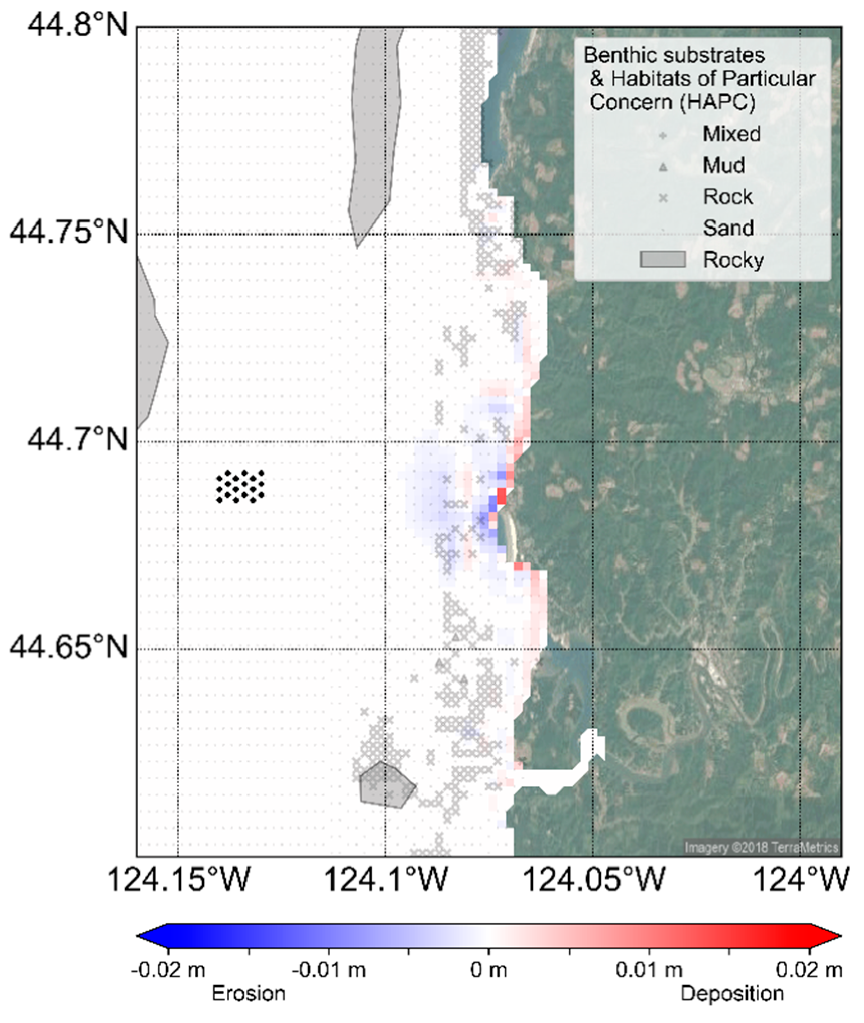
Figure 12 is a map of risk metrics when applied to bottom elevation changes. As discussed in Section 2.3, bottom elevation risk is expressed in changes in bed elevation in units of meters. Changes less than zero meters reflect an erosional environment and changes greater than zero meters reflect a depositional environment. SEAT results indicate that there is generally no change in bed elevation in the majority of the model domain. In regions where bottom elevation risk is non-zero, e.g., in shallow coastal areas, changes in the order of 1 cm are observed. These changes are largely insignificant (<0.5%) when considering that coastal bed elevations are in the order of 5 m.

A quantitative assessment of risk by habitat type is presented in

Table 3. Change in SEAT risk for seabed parameters by habitat type (Equations (7) and (8)).

Habitat	Sediment Mobility Risk (max, non-dim)	Bed Elevation Risk (max, meters)
Estuary	9.38 × 10−7	0.0008
Kelp	0.0009	0.0006
Seagrass	0	0
Rocky	0.0050	1.83 × 10−5
Mixed	5.12 × 10−5	1.04 × 10−5
Mud	−0.0004	8.71 × 10−5
Rock	0.0015	0.0013
Sand	0.0355	0.0132

, which shows the maximum risk of sediment mobility and bed elevation for different habitats found within the model domain. The low numbers suggest that maximum risk values for both sediment mobility and bed elevation are negligible in the presence of WECs. Sediment mobility risk values are very close to zero, noting that regime shifts in sediment mobility occur at ±1 (Equation (7)) and modeled bed changes are generally considerably less than 1 cm. The maximum risk values are in the most dynamic rocky and sandy environments that have high baseline sediment mobility potential.

4. Summary and Conclusions

The present study accomplishes three goals:

• To develop a suitable case study that exemplifies tools and techniques for supporting marine environmental assessments,
• To outline the application of the SEAT at the case study site, and
• To develop maps and tables of WEC-induced stressors and the relationship to sediment transport and seabed changes as determined in the assessment.

The inclusion of sediment parameters in the coupled Delft3D-FLOW-SNL-SWAN model allows for a probabilistic assessment of the effect of WECs on the benthic and coastal environments, forming the basis of the SEAT. The methodology was examined using a subset of wave events, based on long-term site evaluations, which form the typical annual wave climate off the coast of Oregon. The data and results generated by a coupled wave, circulation, and sediment transport model can provide a wealth of information to assess the potential nearshore effects of WECs on hydrodynamics and sediment characteristics. However, the interpretation of the model results may be challenging and subjective. Therefore, the development of a risk assessment tool that utilizes model results, such as the SEAT, may provide a more effective means for coastal resource management.

The SEAT utilizes a holistic approach to site assessments that incorporates a joint probability distribution to capture wave dynamics over the course of a climatological year. Using the occurrence distribution of various wave events based on the analysis of a seven-year wave record, representative discrete wave events were chosen using clustering methodology to reduce the number of discrete wave events to a reasonable number. The clustering method is grounded in the specific wave dynamics in the region of interest, such as typical directional ranges, directional spreading associated with typical swell events, and the variance in significant wave height and period. When taken together, the cumulative sum of discrete wave events formed a climatological set that enabled an evaluation of the spatial risk potential. This probabilistic approach allowed for the calculation of expected changes to parameters such as annual changes in critical shear stress and bed elevation.

The risk metrics presented in this study allow for a spatial characterization of physical risk for several key parameters such as sediment mobility and bed elevation change. These risk metrics for sediment mobility are based on the concept of critical thresholds above which sediment mobilization is likely. The critical threshold for sediment mobility was defined as the critical shear stress of the underlying sediment. The spatial visualization of risk allows for the rapid identification of potential changes to the system and percent changes for parameters in each habitat type allow for a comprehensive evaluation of change. The overall WEC-induced physical stressors risk is very low for the Newport, Oregon case study, with no significant changes in risk that affect sediment mobility or bed elevation change.

The results of the SEAT illustrate the benefits of a site evaluation tool in facilitating coastal resource management at early market WEC sites. Though the SEAT is not intended to replace the traditional environmental assessment process, it can provide important information on potential components of environmental risk. Furthermore, whereas the methodologies shown here were applied to a hypothetical WEC array, these analysis techniques can be applied to other sectors of the renewable energy market such as tidal and offshore wind installations. In addition, risk parameters can be extended to include the effects of marine hydrokinetic energy installations on larval motility or light levels in the context of seagrass sustainability.

References

- Jacobson, P.; Hagerman, G.; Scott, G. Mapping and Assessment of the United States Ocean Wave Energy Resource; Technical Report for Electric Power Research Institute: Palo Alto, CA, USA, December 2011. [Google Scholar]
- Handbook of Ocean Wave Energy; Pecher, A., Kofoed, J.P., Eds.; Springer International Publishing: Basel, Switzerland, 2017; pp. 1–287. [Google Scholar]
- EMEC: European Marine Energy Centre. Available online: http://www.emec.org.uk/marine-energy/wave-developers/ (accessed on 23 July 2018).
- de Sousa Prado, M.G.; Gardner, F.; Damen, M.; Polinder, H. Modelling and test results of the Archimedes wave swing. Proc. IMechE Part A: J. Power Energy, 2006, 220, 855–868. [Google Scholar] [CrossRef]
- Contestabile, P.; Iuppa, C.; Di Lauro, E.; Cavallaro, L.; Andersen, T.L.; Vicinanza, D. Wave loadings acting on innovative rubble mound breakwater for overtopping wave energy conversion. Coast. Eng. 2017, 122, 60–74. [Google Scholar] [CrossRef]
- Cameron, L.; Doherty, R.; Henry, A.; Doherty, K.; Van’t Hoff, J.; Kaye, D.; Naylor, D.; Bourdier, S.; Whittaker, T. Design of the next generation of the Oyster wave energy converter. In Proceedings of the 3rd International Conference on Ocean Energy, Bilbao, Spain, 6–8 October 2010; pp. 1–12. [Google Scholar]
- Nelson, P.A.; Behrens, D.; Castle, J.; Crawford, G.; Gaddam, R.N.; Hackett, S.C.; Largier, J.; Lohse, D.P.; Mills, K.L.; Raimondi, P.T.; Robart, M.; Sydeman, W.J.; Thompson, S.A.; Woo, S. Developing wave energy in coastal California: potential socio-economic and environmental effects. 2008; California Energy Commission. Available online: https://www.energy.ca.gov/2008publications/CEC-500-2008-083/CEC-500-2008-083.PDF (accessed on 5 April 2018).
- Millar, D.; Smith, H.C.M.; Reeve, D.E. Modelling analysis of the sensitivity of shoreline change to a wave farm. Ocean Eng. 2007, 34, 884–901. [Google Scholar] [CrossRef]
- Beels, C.; Troch, P.; De Visch, K.; Kofoed, J.P.; De Backer, G. Application of the time-dependent mild-slope equations for the simulation of wake effects in the lee of a farm of Wave Dragon wave energy converters. Renew. Energy 2010, 35, 1644–1661. [Google Scholar] [CrossRef]
- Haller, M.C.; Özkan-Haller, T. Physical-environmental effects of wave and offshore wind energy extraction: a synthesis of recent oceanographic research. Available online: https://core.ac.uk/download/pdf/10196785.pdf (accessed on 20 April 2018).
- Smith, H.C.M.; Pearce, C.; Millar, D.L. Further analysis of change in nearshore wave climate due to an offshore wave farm: An enhanced case study for the Wave Hub site. Renew. Energy 2010, 40, 51–64. [Google Scholar] [CrossRef]
- Abanades, J.; Greaves, D.; Iglesias, G. Wave farm impact on the beach profile: A case study. Coast. Eng. 2014, 86, 36–44. [Google Scholar] [CrossRef]
- O’Dea, A.M.; Haller, M.C. Analysis of the impacts of wave energy converter arrays on the nearshore wave climate. In Proceedings of the 2nd Marine Energy Technology Symposium, METS2014, Seattle, WA, USA, 15–17 April 2014; pp. 36–44. [Google Scholar]
- Riefolo, L.; Lanfredi, C.; Azzellino, A.; Vicinanza, D. Environmental impact assessment of wave energy converters: A review. In Proceedings of the International Conference on Applied Coastal Research, SCACR 2015, Florence, Italy, 28 September–1 October 2015. [Google Scholar]
- Özkan-Haller, T.; Haller, M.C.; McNatt, J.C.; Porter, A.; Lenee-Bluhm, P. Analyses of wave scattering and absorption produced by WEC arrays: Physical/numerical experiments and model assessment. Mar. Renew. Energy 2017, 71–97. [Google Scholar]
- Watson, J.R.; Hays, C.G.; Raimondi, P.T.; Mirarai, S.; Dong, C.; McWilliams, J.C.; Blanchette, C.A.; Caselle, J.E.; Siegel, D.A. Currents connecting communities: nearshore community similarity and ocean circulation. Ecology 2011, 92, 1193–1200. [Google Scholar] [CrossRef] [PubMed]
- O’Boyle, L.; Elsabet, B.; Whittaker, T. Experimental measurement of wave field variations around wave energy converter arrays. Sustainability 2017, 9, 70. [Google Scholar] [CrossRef]
- Gonzalez-Santamaria, R.; Zou, Q.; Pan, S. Modelling of the impact of a wave farm on nearshore sediment transport. Coast. Eng. Proc. 2012, 1, 66. [Google Scholar] [CrossRef]
- Zanopol, A.T.; Onea, F.; Rusu, E. Coastal impact assessment of a generic wave farm operating in the Romanian nearshore. Energy 2014, 72, 652–670. [Google Scholar] [CrossRef]
- Shih, S.M.; Komar, P.D. Sediments, beach Morphology, and Sea Cliff Erosion within and Oregon Coast Littoral Cell. J. Coast. Res. 1994, 19, 144–157. [Google Scholar]
- Twenhofel, W.H. Minerological and Physical Composition of the Sands of the Oregon Coast from Coos Bay to the Mouth of the Columbia River; Bulletin No. 30; Department of Geology and Mineral Industries: Portland, OR, USA, 1946.
- Federal Geographic Data Committee. Coastal and Marine Ecological Classification Standards (CMECS); June 2016. Available online: https://iocm.noaa.gov/cmecs/ (accessed on 19 June 2018).
- Harlett, J.C.; Kulm, L.D. Suspended sediment transport on the northern Oregon continental shelf. Geol. Soc. Amer. Bull. 1973, 84, 3815–3826. [Google Scholar] [CrossRef]
- Booij, N.; Ris, R.C.; Holthuijsen, L.H. A third-generation wave model for coastal regions. Part I: Model description and validation. J. Geophys. Res. 1999, 104, 7649–7666. [Google Scholar] [CrossRef]
- Delft University of Technology. SWAN User Manual, SWAN Cycle III version 41.01; Delft University of Technology: Delft, The Netherlands, 1993. [Google Scholar]
- Ruehl, K.; Porter, A.; Posner, A.; Roberts, J. Development of SNL-SWAN, a Validated Wave Energy Converter Array Modeling Tool. In Proceedings of the 10th European Wave and Tidal Energy Conference, Aalborg, Denmark, 2–5 September 2013. [Google Scholar]
- Ruehl, K.M.; Chartrand, C.; Porter, A. SNL-SWAN Manual, Version 1.0; SAND Report; Sandia National Laboratories: Albuquerque, NM, USA, 2014.
- Ruehl, K.M.; Porter, A.; Chartrand, C.; Smith, H.; Chang, G.; Roberts, J. Development, Verification and Application of the SNL-SWAN Open Source Wave Farm Code. In Proceedings of the 11th European Wave and Tidal Energy Conference, Nantes, France, 6–11 September 2015; pp. 1–8. [Google Scholar]
- Chang, G.; Ruehl, K.; Jones, C.A.; Roberts, J.; Chartrand, C. Numerical modeling of the effects of wave energy converter characteristics on nearshore wave conditions. Renew. Energy 2016, 89, 636–648. [Google Scholar] [CrossRef]
- Roelvink, J.A.; Van Banning, G.K.F.M. Design and development of DELFT3D and application to coastal morphodynamics. Oceanogr. Lit. Rev. 1995, 42, 925–938. [Google Scholar]
- Gerritsen, H.; deGoede, E.D.; Platze, F.W.; van Kester, J.A.Th.M.; Gensenberger, M.; Uittenbogaard, R.E. Validation Document Delft3D-FLOW, A Software System for 3D Flow Simulations; Deltares: Delft, The Netherlands, 2008. [Google Scholar]
- Egbert, G.D.; Erofeeva, S.Y. Efficient inverse modeling of barotropic ocean tides. J. Atmos. Ocean. Technol. 2002, 19, 183–204. [Google Scholar] [CrossRef]
- García-Medina, G.; Özkan-Haller, H.T.; Ruggiero, P. Wave resource assessment in Oregon and southwest Washington, USA. Renew. Energy 2014, 64, 203–214. [Google Scholar] [CrossRef]
- Kuik, A.J.; vanVledder, G.P.; Holthuijsen, L.H. A method for the routine analysis of pitch-and-roll buoy wave data. J. Phys. Oceanogr. 1988, 18, 1020–1034. [Google Scholar] [CrossRef]
- Bull, D.; Dallman, A. Wave Energy Prize experimental sea state selection. In Proceedings of the OMAE 36th International Conference on Ocean, Offshore and Arctic Engineering, Trondheim, Norway, 25–30 June 2017. [Google Scholar] [CrossRef]
- Lesser, G.R.; Roelvink, J.A.; van Kester, J.A.T.M.; Stelling, G.S. Development and validation of a three-dimensional morphological model. Coast. Eng. 2004, 51, 883–915. [Google Scholar] [CrossRef]
- Soulsby, R.L. Dynamics of Marine Sands—A Manual for Practical Applications; Thomas Telford Publications: London, UK, 1997. [Google Scholar]
- Babarit, A.; Hals, J.; Muliawan, M.J.; Kurniawan, A.; Moan, T.; Krokstad, J. Numerical benchmarking study of a selection of wave energy converters. Renew. Energy 2012, 41, 44–63. [Google Scholar] [CrossRef]
© 2018 by the authors. Licensee MDPI, Basel, Switzerland. This article is an open access article distributed under the terms and conditions of the Creative Commons Attribution (CC BY) license (http://creativecommons.org/licenses/by/4.0/).