A Novel Single-Terminal Fault Location Method for AC Transmission Lines in a MMC-HVDC-Based AC/DC Hybrid System


The Key Laboratory of Smart Grid of Ministry of Education, Tianjin University, Tianjin 300072, China
*
Author to whom correspondence should be addressed.
Energies 2018, 11(8), 2066; https://doi.org/10.3390/en11082066
Submission received: 17 July 2018
/
Revised: 30 July 2018
/
Accepted: 7 August 2018
/
Published: 8 August 2018
(This article belongs to the Special Issue Fault Diagnosis on MV and HV Transmission Lines)
Abstract
:Accurate and reliable fault location method for alternating current (AC) transmission lines is essential to the fault recovery. MMC-based converter brings exclusive non-linear characteristics to AC networks under single-phase-to-ground faults, thus influencing the performance of the fault location method. Fault characteristics are related to the control strategies of the converter. However, the existing fault location methods do not take the control strategies into account, with further study being required to solve this problem. The influence of the control strategies to the fault compound sequence network is analyzed in this paper first. Then, a unique boundary condition that the fault voltage and negative-sequence fault current merely meet the direct proportion linear relationship at the fault point, is derived. Based on these, a unary linear regression analysis is performed, and the fault can be located according to the minimum residual sum function principle. The effectiveness of the proposed method is verified by PSCAD/EMTDC simulation platform. A large number of simulation results are used to verify the advantages on sampling frequency, fault resistance, and fault distance. More importantly, it provides a higher ranging precision and has extensive applicability.
1. Introduction
Modular multilevel converter-based high voltage direct current (MMC-HVDC) plays an increasingly important role in the field of renewable energy integration and regional power grid interconnection, due to its outstanding advantages in having no commutation failure, flexible control, and superior harmonic performance [1]. The world’s first ± 500 kV four-terminal MMC-HVDC demonstration project is currently under construction in Zhangbei, China, which is attracting more research interest in direct current (DC) short-circuit faults. But as an alternating current (AC)/DC hybrid system, the influence of AC faults should not be neglected. The single-phase-to-ground fault is one that happens frequently in AC transmission line, and the short-circuit current will seriously affect the safety and stability of the system. Therefore, locating and clearing the fault point as soon as possible is of great significance to improve the economy and reliability of the system operation [2]. However, the fault transient characteristics of the MMC-based converters in AC sides are influenced by the control strategies, which will cause some difficulties for locating fault [3].
At present, the existing fault location methods for AC transmission lines can be classified into three main categories: traveling wave methods [4,5,6], artificial intelligence-based methods [7,8,9], and impedance-based methods [10,11,12,13,14,15,16,17,18,19]. Based on global positioning system, synchronized transient voltage measurements from double terminals are used to locate the fault in [4]. Reference [5] depends on the time difference between the first incident wave and the successive reflections from the fault point, which provide a method for identifying the reflected wave. In order to exert low computation burden, a method based on the Gabor transform is presented in [6]. Traveling wave methods have proven to have many excellent characteristics, but its limitations are apparent. The requirement of high sampling rate, reflected traveling waves that are hard to identify, and the poor anti-interference capability, will affect the accuracy of fault location. Artificial intelligence-based methods are suitable for handling the uncertainties of power systems. Artificial neural networks and support vector machines are used in [7]. Reference [8] is based on support vector regression, and uses the amplitudes of the single-terminal fault voltage waveforms to locate the fault. In [9], a machine-learning algorithm is proposed. However, these methods depend severely on the training process, and samples are often not available in practice.
For the aspect of impedance-based methods, methods based on two-terminal electrical quantities are introduced in [10,11,12]. The methods might not be feasible due to data synchronization, communication technology, and high investment cost. References [10,11] make efforts to solve the problem of data synchronization, but the iterative computation involved is too complicated. With the development of phasor measurement units, methods based on synchronized phasor is proposed in [12]. Impedance-based methods based on single-terminal electrical quantity calculate the fault location from the apparent impedance [13,14,15,16,17,18,19]. The principle of such methods is simple and easy to implement, but the accuracy is seriously affected by fault resistance and opposite terminal systems. In order to improve the ranging precision, improved methods are introduced in [14,15]. Considering the non-linear characteristics of the arc, the arc voltage is equivalent to the current-controlled square wave source in [16]. The effect of mutual coupling in the double-circuit transmission lines is taken into account in [17,18], which are based on six-sequence components to locate faults. However, the assumption that the current through the fault branch is in phase with the current at the measurement point, is a problem that the methods are unable to avoid. Reference [19] proposes to combine the impedance-based method with the traveling wave method, but this brings new difficulties in algorithm cooperation. In addition, some methods based on wide area measurements are proposed in [20,21]. These methods put forward higher requirements for the development of the future power grid.
To improve the ability of continuous operating, the MMC-based converter adopts a fault ride through control strategy, which displays major differences from traditional AC systems. The control system adjusts the magnitude and phase of the output current in real time, according to the falling degree of the positive-sequence voltage. As a result, the output behavior of the converter is non-linear [22]. Once a serious short-circuit fault occurs at the near end of the converter, and the falling degree of voltage exceeds the capacity of the fault control strategy, the converter will be blocked. Due to the output electrical quantity of the converter cannot be obtained effectively, impedance-based methods based on two-terminal are not suitable. Moreover, the angle between the AC bus voltage and the output current of the converter is no longer equal to the line impedance angle under the fault condition, and it further breaks the in-phase assumption of the single-terminal impedance-based methods. As a result, the methods mentioned above need improvement in order to meet the fault location task for the AC transmission line in MMC-HVDC-based AC/DC hybrid systems [23], and the control strategies of the converter must be considered.
In this paper, the influence of control strategies adopted by the converter is analyzed in detail first. Based on the analysis, a feasible fault location method is proposed to improve the precision of the fault location. Through the proposed method, a single-phase-to-ground fault can be accurately located by single-terminal electrical quantity of the traditional power source side.
The rest of this paper is organized as follows: Section 2 introduces the control system of the MMC-HVDC-based AC/DC hybrid system and analyzes the influence of the negative-sequence current restraint strategy. The principle and criterion of the fault location method are introduced in Section 3. The parameters of the simulation model using PSCAD/EMTDC (X4.5, Manitoba HVDC Research Centre Inc., Winnipeg, MB, Canada) and simulation results of the proposed method are presented in Section 4. Some conclusions are summarized in Section 5.
2. Control System of the AC/DC Hybrid System
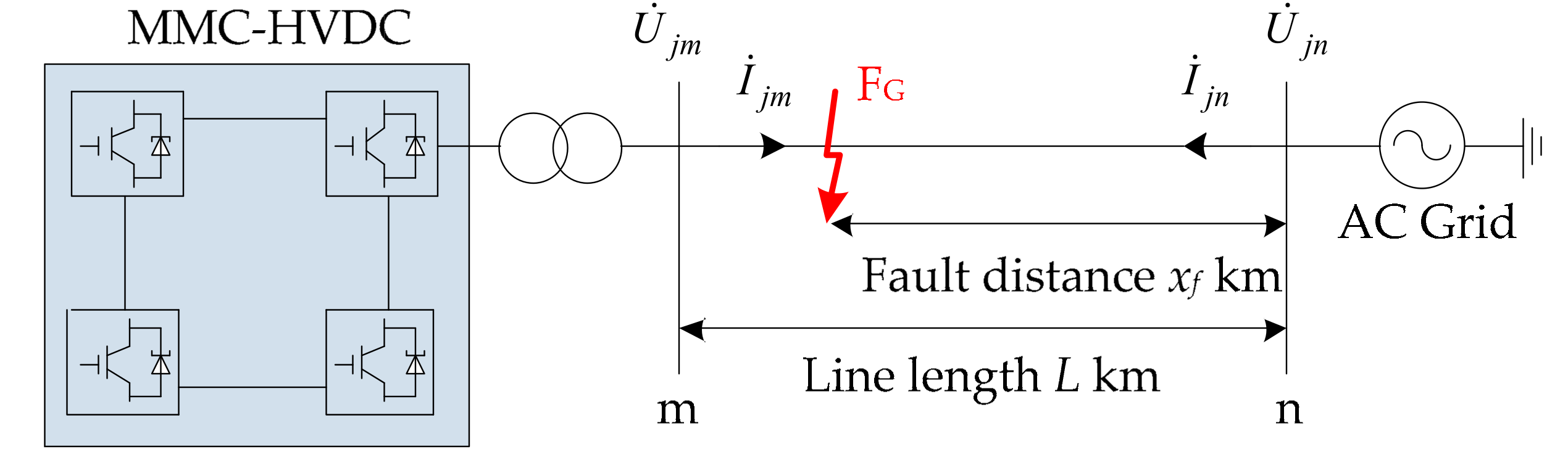
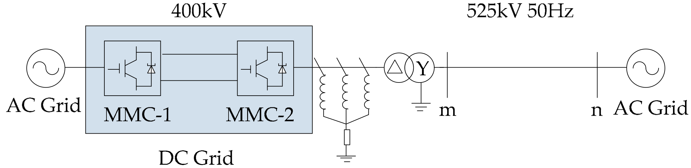
The model of an AC/DC hybrid system is shown in Figure 1, which contains a typical four-terminal MMC-HVDC transmission system [24]. The single-phase-to-ground fault FG arises at the AC transmission line mn, which emanates from the converter. and are the voltage and current phasors, respectively, and j represents three-phase of the line mn (j = A, B and C). The total length of the line is L km and xf denotes a random fault distance from the bus n.
The control system of each MMC-based converter is composed of inner positive-sequence current control loops, inner negative-sequence current control loops, outer power control loops [25], a synchronous d-q frame phase detector [26], and a fault ride through control strategy, and so on.
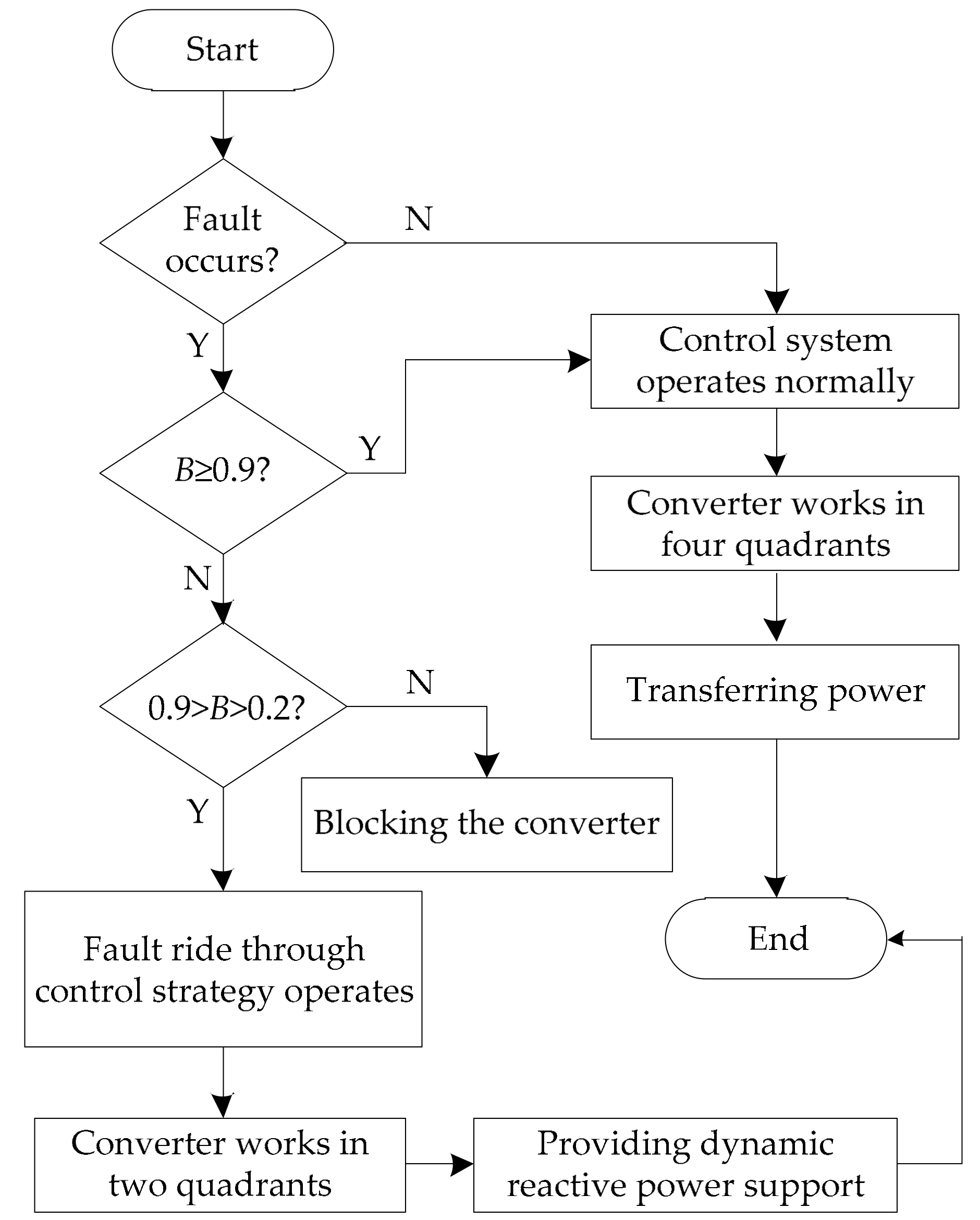
A flowchart of the control system is shown in Figure 2. If there is no fault occurring on the transmission line, the control system of the MMC-based converter will operate normally. The converter can work in all four quadrants of the P–Q operating plane, to realize the function of the power transmission, and the power factor ranges from −1 to 1. If there is a fault and the ratio between the actual positive sequence voltage of the AC bus and the rated voltage B ≥ 0.9, the control system will maintain the same control target as that under normal operation. On the contrary, if 0.9 > B > 0.2, the fault ride through control strategy will operate to adjust the magnitude and phase of the output current [27]. In order to provide dynamic reactive power support for the AC system, the converter will work in two quadrants where Q > 0. In addition, if B < 0.2, converter will be blocked and quit operating.
When the AC system operates under unbalanced conditions, the inner negative-sequence current control loops will eliminate the negative-sequence output current of the fault side converter, to improve the performance of converters and to ensure the security of systems. The command reference of negative-sequence power currents and are set as zero, so that the negative-sequence component of the output current is no longer obvious. This control method is called negative-sequence current restraint strategy [28].
3. The Fault Location Method
3.1. Principle of the Proposed Method
Based on Section 2, when a phase-A-to-ground fault occurs in the line mn and B > 0.2, the fault side converter can rapidly take corresponding control strategies, which will limit the negative-sequence current flowing from the converter close to zero. , which is provided by the converter, is composed of positive- and zero-sequence components, and it can be expressed as . On the contrary, the traditional AC grid side will still generate a negative-sequence component, and can be expressed as .
Therefore, the negative-sequence network of the phase-A-to-ground fault only contains the traditional AC grid side, which constitutes a single-terminal network. The negative-sequence current of the fault point is provided by the traditional AC grid. Thus, it rules out the influence that fault information of the converter side made to the fault point in principle. Based on the above characteristic, accurate fault location adopting the single-terminal electrical quantity of the bus n side can be realized.
According to Figure 1, assuming that the phase-A-to-ground fault occurs with fault grounding resistance Rf. and are the residual voltage of the fault point in phase A, and the current flowing through the fault branch, respectively. Their relationship can be written as Equation (1):
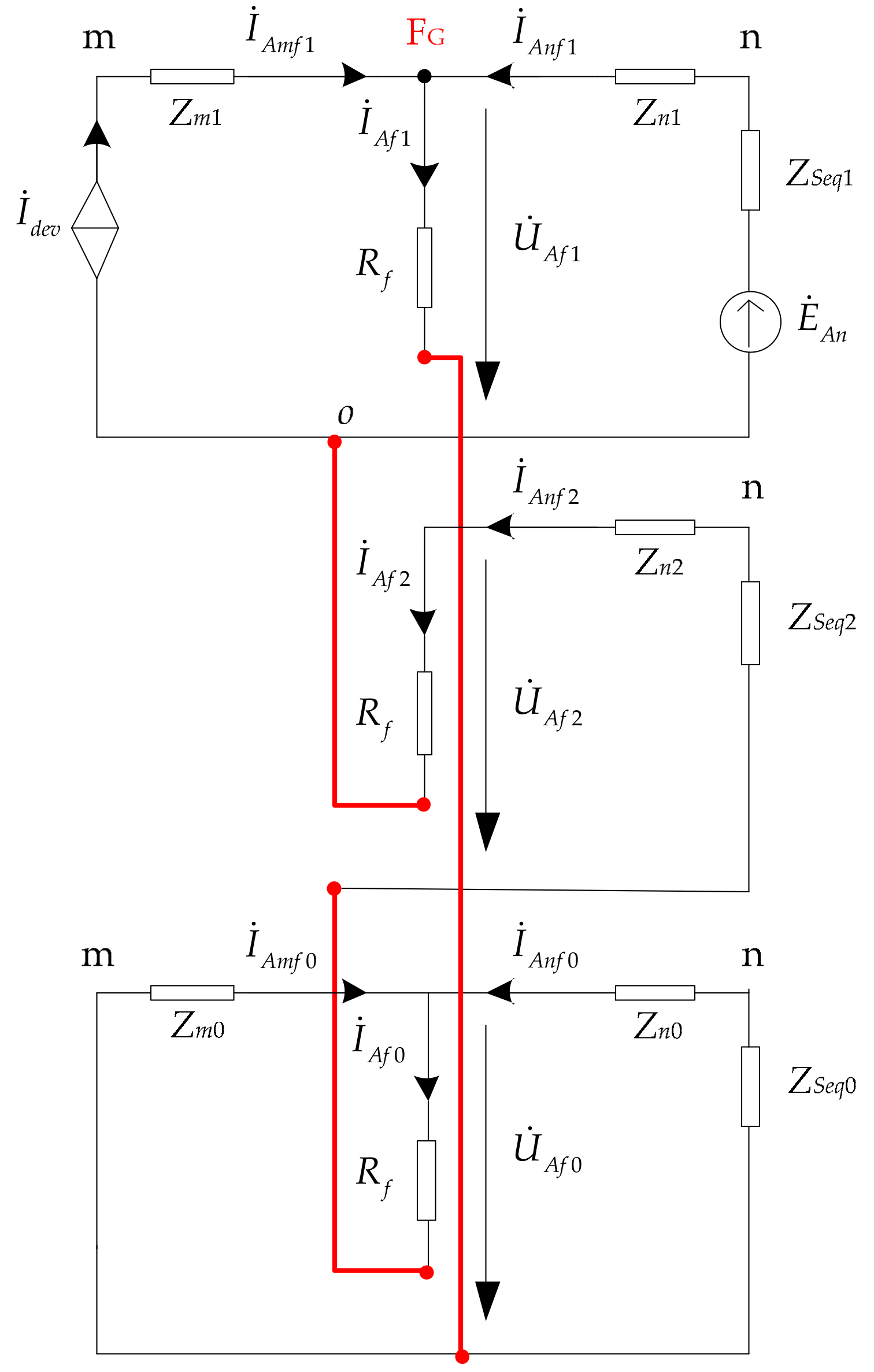
The compound sequence network under the phase-A-to-ground fault is shown in Figure 3, which is the series of positive-, negative-, and zero-sequence networks. The converter and its system behind can be equivalent to a controlled positive-sequence current source , which is not influenced by its working state in a rectifier or inverter [29]. Meanwhile, whatever the fault ride through control strategy adopted by the converter, the equivalence exists. Thus, the fault location method is not influenced by the fault ride through control strategy. Noted that and are the fault sequence component currents at the fault point from the bus m side and n side, respectively. Zm1,0, Zn1,2,0, and ZSeq1,2,0 are the sequence component impedances between the bus m and the fault point, the sequence component impedances between the bus n and the fault point, and the equivalent sequence component impedances of the AC network at the back side of bus n, respectively. The impedance of the converter is neglected in this paper.
The positive-, negative-, and zero-sequence components of the fault branch current meet Equation (2):
where , and .
According to Equations (1) and (2), the boundary condition under the phase-A-to-ground fault at the fault point is:
For a random position in the fault phase line, its fault voltage and negative-sequence fault current only satisfy Equation (3) at the fault point. But in the other positions other than the fault point, due to the influence of the distributed parameter, their relationship is non-linear.
Therefore, the fault location can be realized under Equation (3)’s boundary condition. Fault voltage and negative-sequence fault current distributing along the fault phase line can be calculated based on the single-terminal electrical quantity of the bus n side. The analysis above is based on B > 0.2. If B < 0.2, the converter will be blocked and cease from operating. The negative-sequence network of the phase-A-to-ground fault is a single-terminal network, and Equation (3)’s boundary condition still exists. Thus, fault location can be realized as long as the fault occurs.
3.2. Criterion of the Proposed Method
According to the analysis above, the data set (, , where i represents different times), locating x off the bus n side, consists of the fault voltage and negative-sequence fault current. It meets the direct proportion linear relationship merely at the fault point.
A direct proportion linear model is established as follow:
The residual sum function H(x) is introduced:
According to the least squares method, to achieve the minimum H(x), the proportional coefficient can be calculated as:
As a consequence, by performing a unary linear regression analysis of the data set, using Equations (5) and (6), the residual sum function H(x) of the whole line can be calculated. The higher the fitting degree between the data set and Equation (4) is, the smaller H(x) will be. The factors affecting the accuracy of the fault location method include the transient process of the converter control system restraining its negative-sequence output current, the rounding error in the process of calculating the fault voltage and negative-sequence fault current, the calculation error in the linear regression analysis, and the current transformer error in the practical application, etc. It is a principle that H(x) is minimum at the fault point, and therefore the fault distance can be located according to the fault location criterion Equation (7):
3.3. Calculation Method for the Fault Voltage and the Negative-Sequence Fault Current
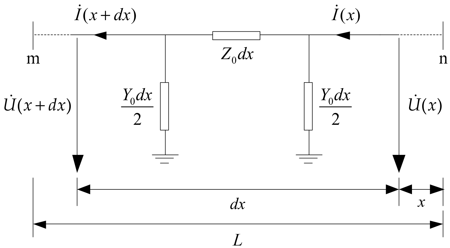
The fault location method is based on the fault voltage and negative-sequence fault current distribution along the fault phase line. In this section, a specific calculation method will be given. The distributed parameter model of a single transmission line is shown in Figure 4, where is the series impedance per unit length of the line, and is the shunt admittance per unit length of the line.
For an infinitesimal section dx, which is located at x from the bus n side, the relationship between the voltage and current can be defined as:
According to single-terminal electrical quantity of the bus n side, Equation (9) can be obtained from Equation (8):
where and are the fundamental frequency voltage and current phasor of the bus n side, respectively, x is the distance between the calculating point and the bus n, is the characteristic impedance of the line, and is the propagation constant.
Electromagnetic induction exists in a three-phase transmission line, which will affect the calculating accuracy of the voltage and current distribution along the line. Thus, before substitution into Equation (9), it is necessary to convert electric quantity of the bus n side into independent modulus components, through a decoupling transformation matrix. The symmetrical component method is one of the most common decoupling transformation matrixes in fault analysis, and the positive-, negative-, and zero-sequence components resulting from the decomposition are independent. A symmetrical component transformation matrix is shown as Equation (10):
For each sequence component, Equation (9) can be written as Equation (11):
where p represents the corresponding sequence component (p = 1, 2 and 0).
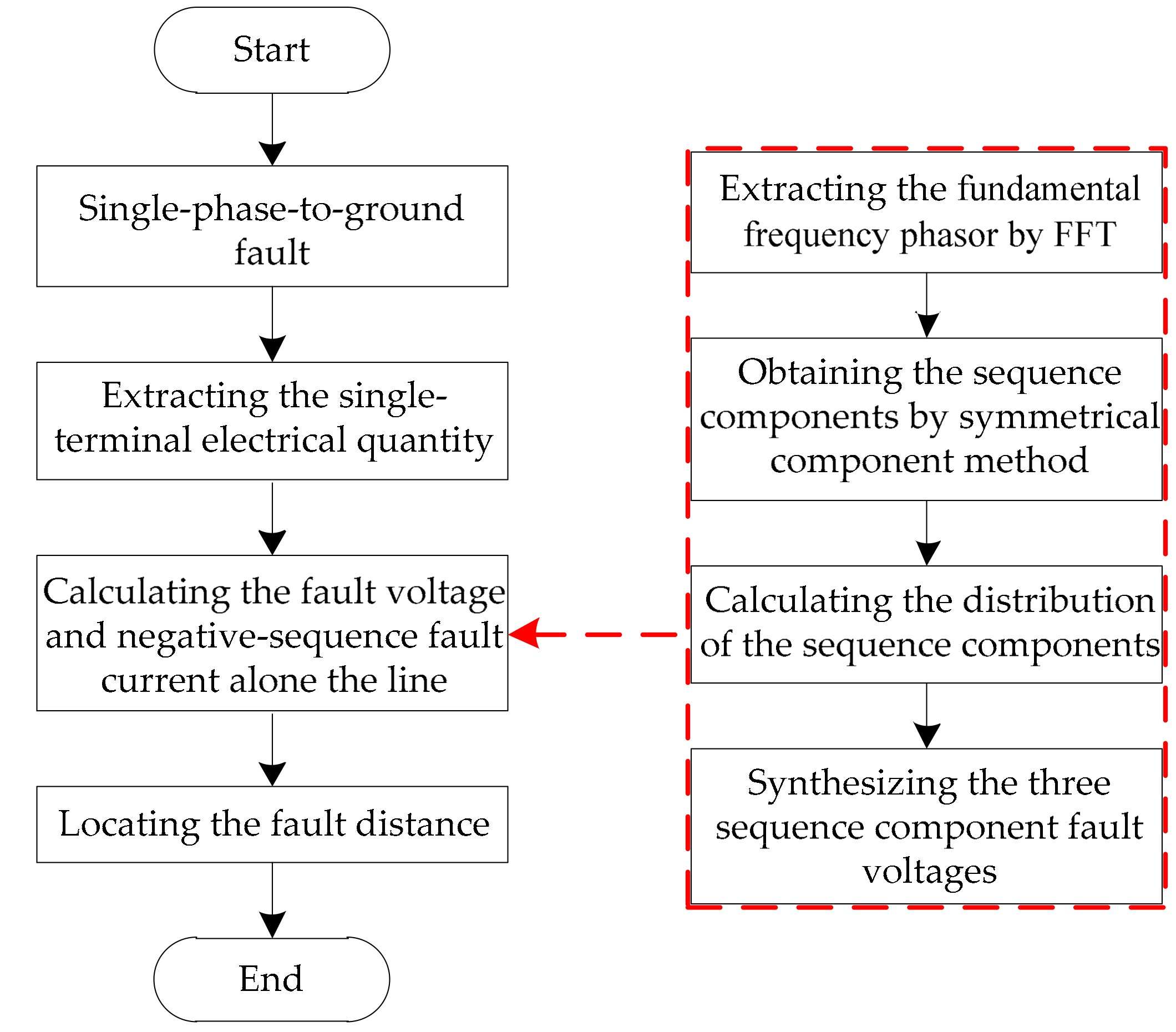
In conclusion, in terms of the distributed parameter, the calculation method of the fault voltage and the negative-sequence fault current distribution along the fault phase line is proposed as follows:
- The fundamental frequency electrical quantity can be extracted from the bus n side by fast fourier transform with a window of sampling data.
- In the frequency domain, the symmetrical component method is used to obtain the sequence components of the fault voltage and fault current.
- Under the sequence component, the line parameters corresponding to the sequence components are substituted into Equation (11), respectively. As a result, the distribution of negative-sequence fault current, positive-, negative-, and zero-sequence fault voltages in the fault phase along the line can be calculated.
- By using the phase-model reverse transformation matrix, the three sequence component fault voltages are synthesized into the fault phase voltage.
3.4. The Process of the Fault Location Method
The overall flowchart of the proposed fault location method is shown in Figure 5. The concrete steps are described as follows:
- The single-phase-to-ground fault can be detected through the protection method proposed in [27], and the fault phase can also be selected.
- The single-terminal electrical quantity of the traditional power source side is extracted.
- The fault voltage and the negative-sequence fault current distributing along the fault phase line are calculated by the method introduced in Section 3.3.
- In the time domain, a data set is obtained, which consists of the fault voltage and the negative-sequence fault current at different times, for each distance along the fault phase line, and the criterion introduced in the Section 3.2 is used to locate the fault distance.
4. Simulation and Verification
4.1. Case Study
Through the analysis in Section 3, we can find that, whether the DC side is a two-terminal or multi-terminal MMC-HVDC transmission system, or whether the DC side adopts a symmetric monopole or a symmetric bipolar connection mode, the fault location method proposed in this paper is applicable.
In order to verify the effectiveness of the fault location method, a typical AC/DC hybrid system simulation model was built on the PSCAD/EMTDC simulation platform, which is shown in Figure 6. The specific parameters of the test model are listed in Table 1, and the fault location algorithm was tested with MATLAB (R2013b, MathWorks, Natick, MA, USA). The converter transformer adopted a Yn/Δ connection mode, and the Δ side of the transformer adopted the small fault current grounding method, which contains star-connected reactors with high grounding resistance [30]. The transmission line adopted the distributed parameter model. The control mode of MMC-1 was constant DC voltage and constant reactive power control, and MMC-2 possessed constant active power and constant reactive power control.
4.2. Simulation Results
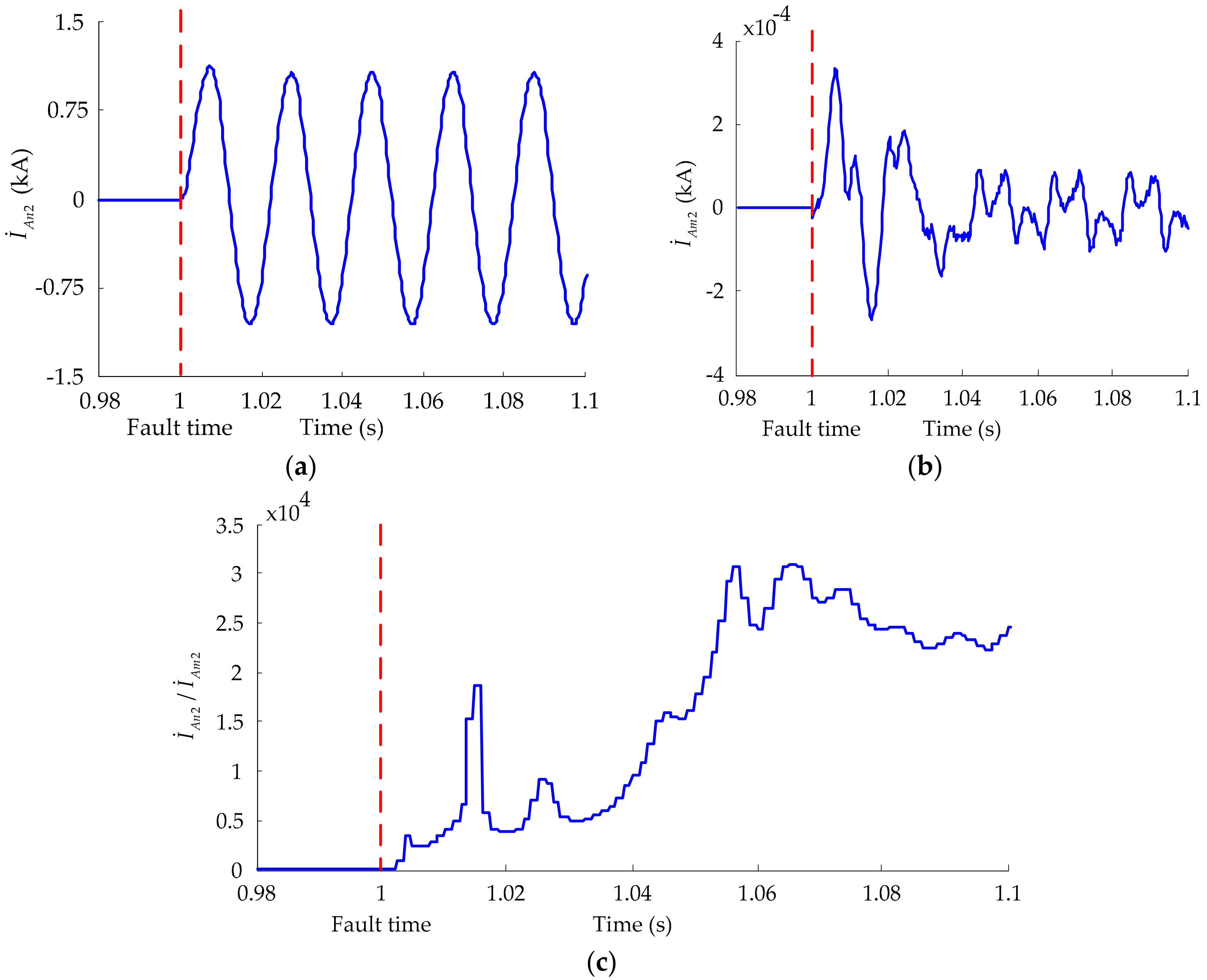
A phase-A-to-ground fault with 100 Ω fault resistance occurred in the line mn at 1 s, and the distance between the fault point and the bus n was 218 km.
The simulation results of negative-sequence fault currents at both sides and their ratio are shown in Figure 7. As shown in Figure 7b, due to the influence of the negative-sequence current restraint strategy, the negative-sequence fault current flowing from the bus m was suppressed quickly. A transient process existed when reduced to zero. It can be seen from Figure 7c, was much bigger than . After 20 ms from the fault inception, their ratio was nearly 5000 and still increasing. Thus, compared with , could be ignored, which verified the rationality of the analysis in Section 3.1.
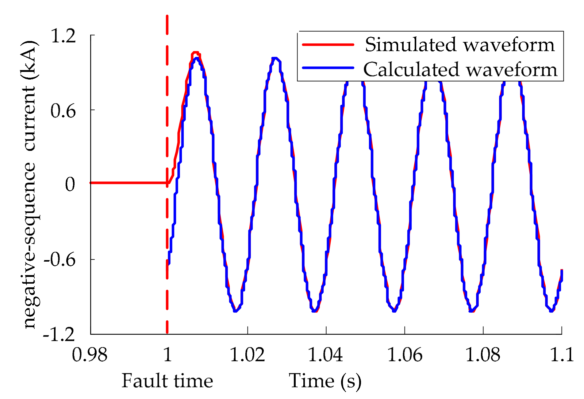
Figure 8 shows the comparison between the calculated negative-sequence current waveform obtained by Equation (11) and the simulated waveform at the fault point. It can be seen that nearly no errors were observed between them at the steady state, which verified the validity of the calculation method proposed in Section 3.3.
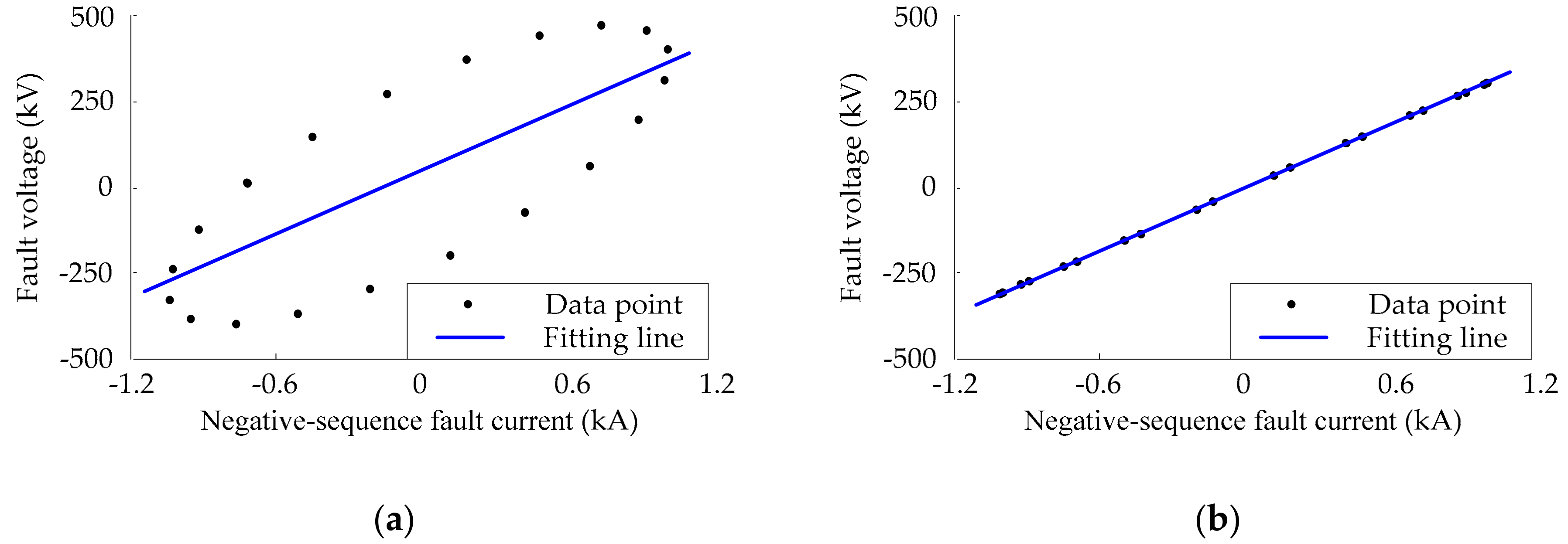
Fitting results between the data set and (4) at the starting point of the line (the bus n) as well as the fault point are shown in Figure 9. As displayed in Figure 9a, the fitting result performed badly at the starting point, making H(x) bigger. But it can be seen from Figure 9b that a high fitting precision was achieved at the fault point, and that the curve slope was about three times the fault resistance, which was consistent with the previous theoretical analysis.
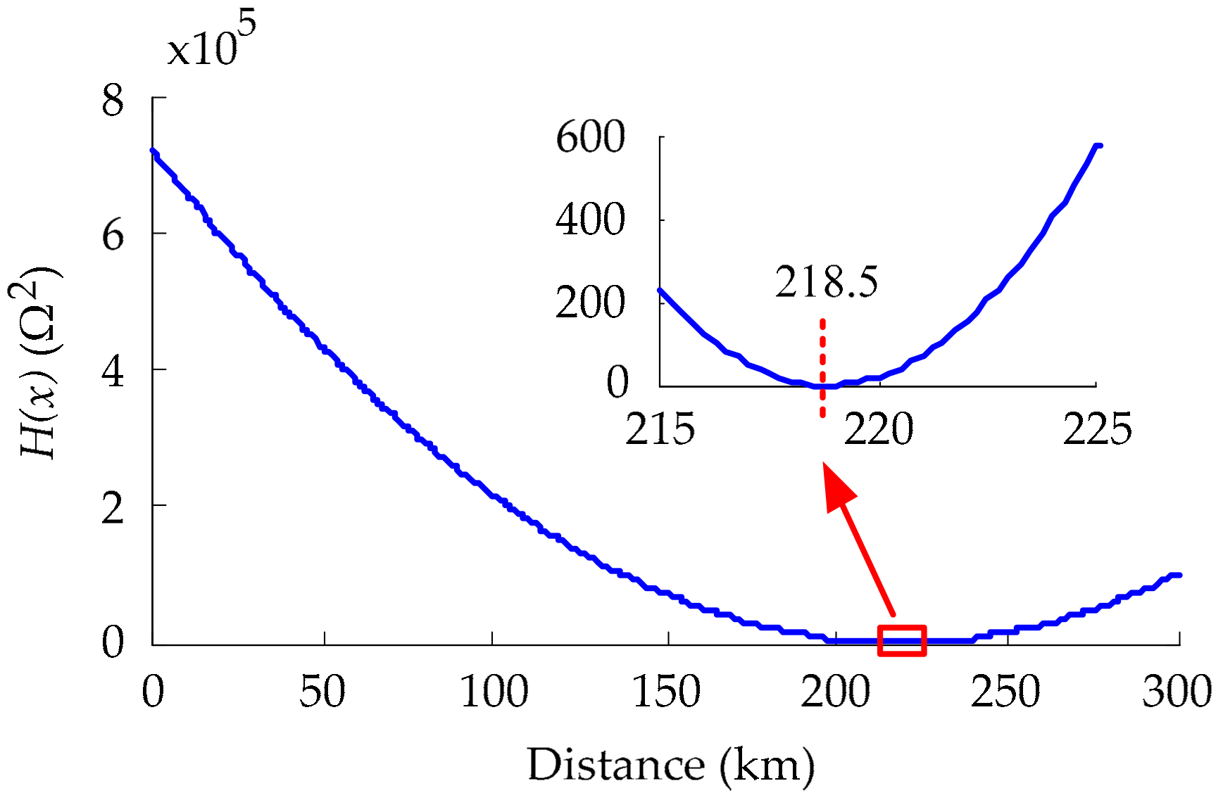
The fault location result is shown in Figure 10. The horizontal axis in the figure represents the distance from the bus n, and the vertical axis represents H(x). It can be seen that the value of H(x) is minimum at 218.5 km, and that the absolute error of fault location is 0.5 km. The result shows that the ranging precision is high, which verifies the feasibility of the fault location method.
4.3. Performance Evaluation
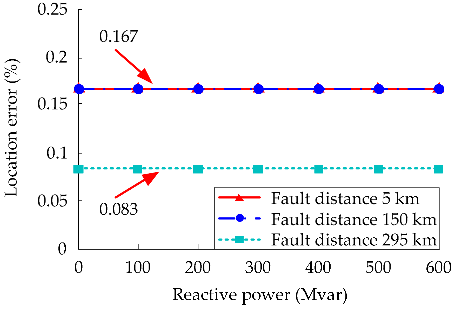
In order to provide dynamic reactive power support for the AC system, fault ride through control strategy of the converter will operate to adjust the magnitude and phase of the output current, which may affect the ranging precision of the fault location method. The simulation results with a different output reactive power of the converter when a single-phase-to-ground fault with 100 Ω fault resistance occurred at 5 km, 150 km, and 295 km of the transmission line were compared in Figure 11. As the figure shows, the location error did not vary with the output reactive power of the converter, which verified that the proposed method had a good fault location performance.
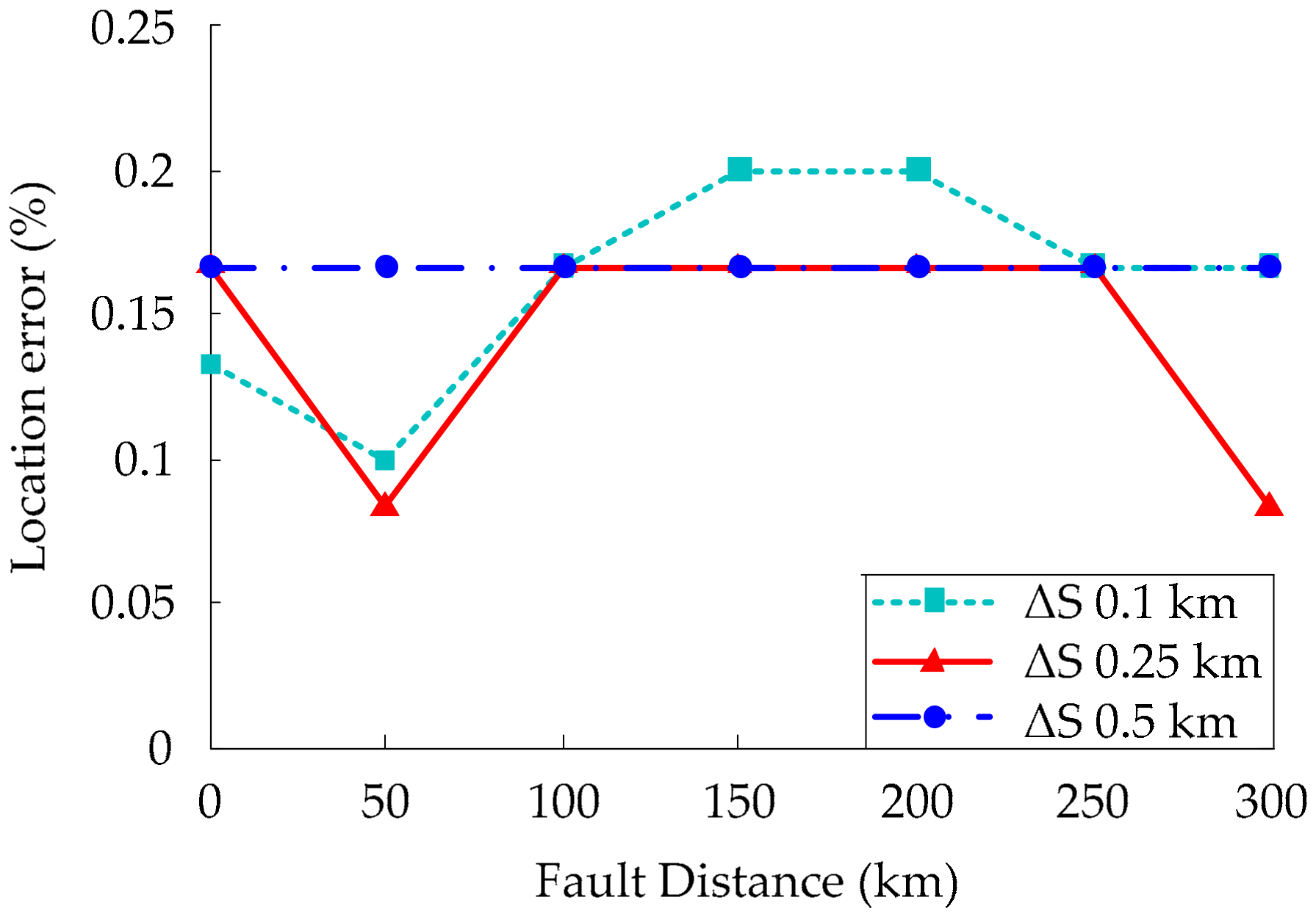
In principle, the more intensive the calculating step ΔS of the fault voltage and negative-sequence fault current along the line is, the higher the ranging precision will be. However, intensive ΔS will also affect the calculating speed of the fault location algorithm. The ranging precision is more valued when conflict occurs. The simulation results with different calculating steps when a single-phase-to-ground fault with 100 Ω fault resistance occurred at different positions of the transmission line, are shown in Figure 12. It can be seen that the location errors were close. In order to improve the calculating speed and ensure accuracy, ΔS was suggested as 0.25 km in the actual project.
The influence of sampling frequency was also taken into account. Table 2 shows the simulation results with different sampling frequencies when a single-phase-to-ground fault with 100 Ω fault resistance occurred at 5 km, 150 km, and 295 km of the transmission line. As shown, the fault location error was not significantly affected, even for a low sampling frequency of 1 kHz. Thus, the proposed method was independent of sampling frequency, making it more practical in implementation.
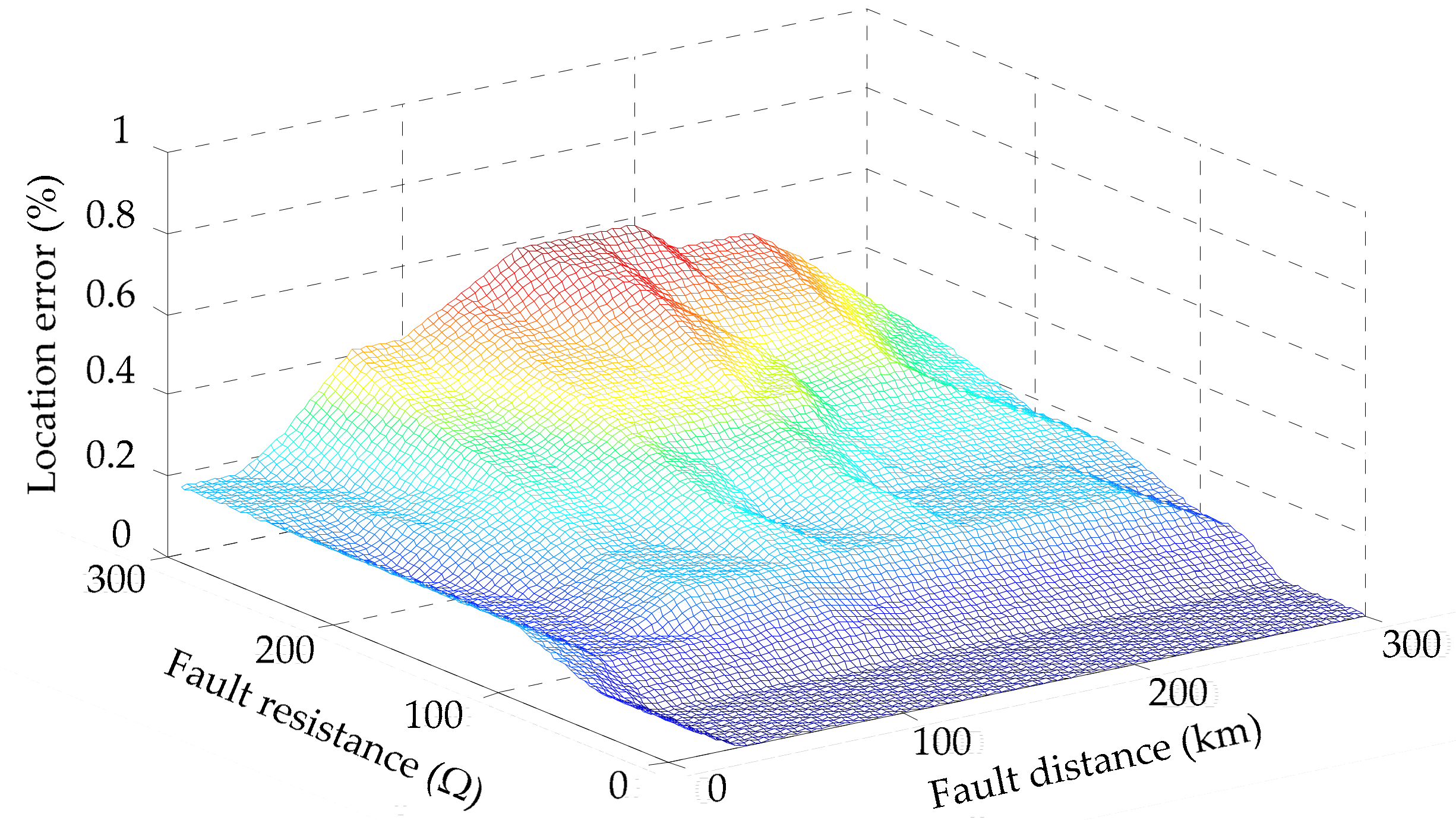
In order to further verify the effectiveness and accuracy of the fault location method, Figure 13 illustrates the fault location error under the single-phase-to-ground fault, with different resistances and different distances. The fault location error = |actual fault distance − calculated fault distance|/total line length × 100%.
It is obvious that within the full length of the line mn, the proposed fault location method detected accurate fault location, and the fault location error was less than 0.6%. The fault location error was not affected by fault distance, but increased as the fault resistance increased. Even so, the fault location method had a strong capability to resist the fault resistance, and it had a high precision even when the fault resistance reached 300 Ω.
Table 3 shows some specific data of Figure 13. What is notable is that due to the calculating step adopted in the paper being 0.25 km, the interval of fault location error was 0.083%. This verifies that the proposed fault location method could maintain good performance irrespective of the fault distance and fault resistance.
5. Conclusions
A novel single-terminal fault location method considering the influence of the control strategies to the fault compound sequence network was proposed in this paper. It is based on the unique boundary condition at the fault point provided by the negative-sequence current restraint strategy of the converter. The fault location method proposed in this paper has the following advantages:
- It solves the problem that the traditional fault location methods are not applicable.
- It is not affected by specific fault ride through control strategy of the MMC-based converter.
- It has a high ranging precision, which is hardly affected by fault resistance, fault distance, sampling frequency, and the distributed capacitance of the line.
- It has extensive applicability, which is applicable to the AC transmission line with a traditional power source, and an MMC-based converter that adopts a negative-sequence current restraint strategy, or voltage source converter-interfaced distributed generators.
Investigation using a real power system will be further conducted to confirm the performance of the proposed fault location method. Further research may lead to method improvements in order to reduce location errors under high fault resistances. In addition, the single-terminal fault location method for other fault types is also our focus.
Author Contributions
S.X. and J.L. put forward the idea and theoretical verification. S.X. conceived and designed the simulation model. J.L. performed the simulation and drafted the article. Valuable comments on the first draft were received from C.L., Y.S., B.L. and C.G.
Funding
This research was funded by The National Key Research and Development Program of China (Grant No. 2016YFB0900901) and the National High Technology Research and Development Program (863 program) of China (No. 2015AA050102).
Acknowledgments
We acknowledge the help of Ruochen An for the English polish.
Conflicts of Interest
The authors declare no conflict of interest.
Nomenclature
The following nomenclatures are used in this manuscript:
| MMC-HVDC | Modular multilevel converter based high voltage direct current |
| FG | Single-phase-to-ground fault |
| The voltage phasor of the bus | |
| The current phasor flowing from the bus | |
| B | The ratio between the actual positive sequence voltage of the AC bus and the rating |
| L | The total length of the line mn |
| xf | Random fault distance from the bus n. |
| The command reference of the negative-sequence active power current | |
| The command reference of the negative-sequence reactive power current | |
| The current flowing from the bus m under a phase-A-to-ground fault | |
| The positive- and zero-sequence components of | |
| The current flowing from the bus n under a phase-A-to-ground fault | |
| The positive-, negative- and zero-sequence components of | |
| Rf | Fault grounding resistance |
| The residual voltage of the fault point in phase A | |
| The current flowing through the fault branch in phase A | |
| The output current of the controlled positive-sequence current source | |
| The fault sequence components current at the fault point from the bus m side | |
| The fault sequence components current at the fault point from the bus n side | |
| Zm1,0 | The sequence impedances between the bus m and the fault point |
| Zn1,2,0 | The sequence impedances between the bus n and the fault point |
| ZSeq1,2,0 | The equivalent sequence impedances of the AC network at the back side of bus n |
| The fault voltage data set | |
| The negative-sequence fault current data set | |
| H(x) | The residual sum function |
| The proportional coefficient | |
| The series impedance per unit length of the line | |
| The shunt admittance per unit length of the line | |
| dx | An infinitesimal section |
| The fundamental frequency voltage phasor of the bus n | |
| The fundamental frequency current phasor of the bus n | |
| The characteristic impedance of the line | |
| The propagation constant | |
| TS | Symmetrical component transformation matrix |
| ΔS | The calculating step |
| The ratio between negative-sequence currents flowing from both sides |
References
- Debnath, S.; Qin, J.; Bahrani, B.; Saeedifard, M.; Barbosa, P. Operation, control, and applications of the modular multilevel converter: A review. IEEE Trans. Power Electron. 2014, 30, 37–53. [Google Scholar] [CrossRef]
- Institute of Electrical and Electronics Engineers (IEEE). IEEE Guide for Determining Fault Location on AC Transmission and Distribution Lines; IEEE Std.: New York, NY, USA, 2015. [Google Scholar]
- Shi, X.; Wang, Z.; Liu, B.; Liu, Y.; Tolbert, L.M.; Wang, F. Characteristic investigation and control of a modular multilevel converter-based HVDC system under single-line-to-ground fault conditions. IEEE Trans. Power Electron. 2014, 30, 408–421. [Google Scholar] [CrossRef]
- Hamidi, R.J.; Livani, H. Traveling-wave-based fault-location algorithm for hybrid multiterminal circuits. IEEE Trans. Power Deliv. 2017, 32, 135–144. [Google Scholar] [CrossRef]
- Lopes, F.V.; Dantas, K.M.; Silva, K.M.; Costa, F.B. Accurate two-terminal transmission line fault location using traveling waves. IEEE Trans. Power Deliv. 2018, 33, 873–880. [Google Scholar] [CrossRef]
- Moravej, Z.; Movahhedneya, M.; Pazoki, M. Gabor transform-based fault location method for multi-terminal transmission lines. Measurement 2018, 125, 667–679. [Google Scholar] [CrossRef]
- Thukaram, D.; Khincha, H.P.; Vijaynarasimha, H.P. Artificial neural network and support vector machine approach for locating faults in radial distribution systems. IEEE Trans. Power Deliv. 2005, 20, 710–721. [Google Scholar] [CrossRef]
- Fei, C.G.; Qi, G.Y.; Li, C.X. Fault location on high voltage transmission line by applying support vector regression with fault signal amplitudes. Electr. Power Syst. Res. 2018, 160, 173–179. [Google Scholar] [CrossRef]
- Chen, Y.Q.; Fink, O.; Sansavini, G. Combined fault location and classification for power transmission lines fault diagnosis with integrated feature extraction. IEEE Trans. Ind. Electron. 2018, 65, 561–569. [Google Scholar] [CrossRef]
- Elsadd, M.A.; Abdelaziz, A.Y. Unsynchronized fault-location technique for two- and three-terminal transmission lines. Electr. Power Syst. Res. 2018, 158, 228–239. [Google Scholar] [CrossRef]
- Hinge, T.; Dambhare, S. Synchronised/unsynchronised measurements based novel fault location algorithm for transmission line. IET Gener. Transm. Distrib. 2018, 12, 1493–1500. [Google Scholar] [CrossRef]
- Deng, Y.; He, Z.; Fu, L.; Lin, S.; Liu, L.; Zhang, J. Research on fault location scheme for inverter AC transmission line of AC–DC hybrid system. IEEJ Trans. Electr. Electron. 2018, 13, 455–462. [Google Scholar] [CrossRef]
- Sachdev, M.S.; Baribeau, M.A. A new algorithm for digital impedance relays. IEEE Trans. Power App. Syst. 1979, 98, 2232–2240. [Google Scholar] [CrossRef]
- Adu, T. A new transmission line fault locating system. IEEE Trans. Power Deliv. 2001, 16, 498–503. [Google Scholar] [CrossRef]
- Farshad, M.; Sadeh, J. Accurate single-phase fault-location method for transmission lines based on k-nearest neighbor algorithm using one-end voltage. IEEE Trans. Power Deliv. 2012, 27, 2360–2367. [Google Scholar] [CrossRef]
- Radojevic, Z.M.; Shin, J.R. New one terminal digital algorithm for adaptive reclosing and fault distance calculation on transmission lines. IEEE Trans. Power Deliv. 2006, 21, 1231–1237. [Google Scholar] [CrossRef]
- Ramar, K.; Low, H.S.; Ngu, E.E. One-end impedance based fault location in double-circuit transmission lines with different configurations. Int. J. Electr. Power Energy Syst. 2015, 64, 1159–1165. [Google Scholar] [CrossRef]
- Tian, B.; Li, Z.X.; Yao, Y.; Wang, L.; Wang, X. Six-sequence component based single ended fault location method of transmission line. In Proceedings of the 2016 International Conference on Electrical Engineering and Automation (ICEEA 2016), Xiamen, China, 18–19 December 2016. [Google Scholar]
- Wang, B.; Dong, X.; Lan, L.; Xu, F. Novel location algorithm for single-line-to-ground faults in transmission line with distributed parameters. IET Gener. Transm. Distrib. 2013, 7, 560–566. [Google Scholar] [CrossRef]
- Das, S.; Singh, S.P.; Panigrahi, B.K. Transmission line fault detection and location using wide area measurements. Electr. Power Syst. Res. 2017, 151, 96–105. [Google Scholar] [CrossRef]
- Dobakhshari, A.S. Wide-area fault location of transmission lines by hybrid synchronized/unsynchronized voltage measurements. IEEE Trans. Smart Grid 2018, 9, 1869–1877. [Google Scholar] [CrossRef]
- Leon, A.E.; Mauricio, J.M.; Solsona, J.A.; Gomez-Exposito, A. Adaptive control strategy for VSC-based systems under unbalanced network conditions. IEEE Trans. Smart Grid 2010, 1, 311–319. [Google Scholar] [CrossRef]
- Chen, K.; Huang, C.; He, J. Fault detection, classification and location for transmission lines and distribution systems: A review on the methods. High Volt. 2016, 1, 25–33. [Google Scholar] [CrossRef]
- Ahmed, N.; Angquist, L.; Mahmood, S.; Antonopoulos, A.; Harnefors, L.; Norrga, S.; Nee, H.P. Efficient modeling of an MMC-based multiterminal DC system employing hybrid HVDC breakers. IEEE Trans. Power Deliv. 2015, 30, 1792–1801. [Google Scholar] [CrossRef]
- Song, H.S.; Nam, K. Dual current control scheme for PWM converter under unbalanced input voltage conditions. IEEE Trans. Ind. Electron. 1999, 46, 953–959. [Google Scholar] [CrossRef]
- Lee, S.J.; Kang, J.K.; Sul, S.K. A new phase detecting method for power conversion systems considering distorted conditions in power system. In Proceedings of the IEEE Industry Applications Conference: Thirty-Fourth IAS Annual Meeting, Phoenix, AZ, USA, 3–7 October 1999. [Google Scholar]
- Xue, S.; Yang, J.; Chen, Y.; Wang, C.; Shi, Z.; Cui, M.; Li, B. The applicability of traditional protection methods to lines emanating from VSC-HVDC interconnectors and a novel protection principle. Energies 2016, 9, 400. [Google Scholar] [CrossRef]
- Guan, M.; Xu, Z. Modeling and control of a modular multilevel converter-based HVDC system under unbalanced grid conditions. IEEE Trans. Power Electron. 2012, 27, 4858–4867. [Google Scholar] [CrossRef]
- Xue, S.; Shi, Z.; Huang, R.; Chang, Q.; Lu, J.; Yang, J. A criterion for non-voltage directional elements applied in AC networks connected with VSC-based interconnection devices. IEEE Trans. Power Electron. 2017, 13, 143–149. [Google Scholar] [CrossRef]
- Hu, J.; Xu, K.; Lin, L.; Zeng, R. Analysis and enhanced control of hybrid-MMC-based HVDC systems during asymmetrical DC voltage faults. IEEE Trans. Power Deliv. 2017, 32, 1394–1403. [Google Scholar] [CrossRef]
Figure 1.
Model of a MMC-HVDC-based AC/DC hybrid system.

Figure 2.
Flowchart of the control system of the MMC-based converter.

Figure 3.
Compound sequence network under the phase-A-to-ground fault of the hybrid system.

Figure 4.
Distributed parameter model.

Figure 5.
Overall flowchart of the proposed fault location method.

Figure 6.
A typical AC/DC hybrid system simulation model.

Figure 7.
Simulation results of the negative-sequence fault currents under the phase-A-to-ground fault: (a) Negative-sequence fault current flowing from the bus n; (b) Negative-sequence fault current flowing from the bus m; (c) The ratio between negative-sequence currents.
Figure 7.
Simulation results of the negative-sequence fault currents under the phase-A-to-ground fault: (a) Negative-sequence fault current flowing from the bus n; (b) Negative-sequence fault current flowing from the bus m; (c) The ratio between negative-sequence currents.

Figure 8.
Comparison between the calculated negative-sequence current waveform and the simulated waveform at the fault point under the phase-A-to-ground fault.
Figure 8.
Comparison between the calculated negative-sequence current waveform and the simulated waveform at the fault point under the phase-A-to-ground fault.

Figure 9.
Fitting results of the fault voltage and negative-sequence fault current under the phase-A-to-ground fault: (a) Starting point of the line; (b) Fault point of the line.
Figure 9.
Fitting results of the fault voltage and negative-sequence fault current under the phase-A-to-ground fault: (a) Starting point of the line; (b) Fault point of the line.

Figure 10.
Location result under the phase-A-to-ground fault.

Figure 11.
Location error with different output reactive power.

Figure 12.
Location error with different calculating steps.

Figure 13.
Location error with different resistances and different distances.


Table 1.
Simulation parameters of the test model.
| System Parameter | Parameter Value |
|---|---|
| DC Voltage/kV | ±400 |
| AC Voltage/kV | 525 |
| Transformer ratio | 525/380 |
| Rated transmission power/MVA | 1000 |
| System frequency/Hz | 50 |
| Grounding electrode resistance/Ω | 1000 |
| Grounding electrode inductance/H | 3 |
| Transmission line length/km | 300 |
| Positive-sequence resistance/(Ω/km) | 0.034676 |
| Positive-sequence inductance/(mH/km) | 1.347616 |
| Positive-sequence capacitance/(nF/km) | 8.6771 |
| Zero-sequence resistance/(Ω/km) | 0.300023 |
| Zero-sequence inductance/(mH/km) | 3.63714 |
| Zero-sequence capacitance/(nF/km) | 6.16105 |
| Sampling frequency/kHz | 3.2 |
| Sampling time/ms | 10 |
| Calculation step ΔS/km | 0.25 |
Table 2.
Location error with different sampling frequencies.
| Actual Fault Distance/km | Sampling Frequency/kHz | Calculated Fault Distance/km | Fault Location Error/% |
|---|---|---|---|
| 5 | 1 | 5.50 | 0.167 |
| 3.2 | 5.50 | 0.167 | |
| 5 | 5.50 | 0.167 | |
| 150 | 1 | 150.50 | 0.167 |
| 3.2 | 150.50 | 0.167 | |
| 5 | 150.50 | 0.167 | |
| 295 | 1 | 295.25 | 0.083 |
| 3.2 | 295.25 | 0.083 | |
| 5 | 295.25 | 0.083 |
Table 3.
Partial results of the location error with different resistances and different distances.
| Actual Fault Distance/km | Fault Resistance/Ω | Calculated Fault Distance/km | Fault Location Error/% |
|---|---|---|---|
| 5 | 0 | 5.25 | 0.083 |
| 100 | 5.50 | 0.167 | |
| 300 | 5.50 | 0.167 | |
| 50 | 0 | 50.00 | 0.000 |
| 100 | 50.25 | 0.083 | |
| 300 | 50.75 | 0.250 | |
| 100 | 0 | 100.00 | 0.000 |
| 100 | 100.50 | 0.167 | |
| 300 | 101.25 | 0.417 | |
| 150 | 0 | 150.00 | 0.000 |
| 100 | 150.50 | 0.167 | |
| 300 | 151.75 | 0.583 | |
| 200 | 0 | 200.00 | 0.000 |
| 100 | 200.50 | 0.167 | |
| 300 | 201.75 | 0.583 | |
| 250 | 0 | 250.00 | 0.000 |
| 100 | 250.50 | 0.167 | |
| 300 | 251.50 | 0.500 | |
| 295 | 0 | 295.00 | 0.000 |
| 100 | 295.25 | 0.083 | |
| 300 | 295.75 | 0.250 |
© 2018 by the authors. Licensee MDPI, Basel, Switzerland. This article is an open access article distributed under the terms and conditions of the Creative Commons Attribution (CC BY) license (http://creativecommons.org/licenses/by/4.0/).
Share and Cite
MDPI and ACS Style
Xue, S.; Lu, J.; Liu, C.; Sun, Y.; Liu, B.; Gu, C. A Novel Single-Terminal Fault Location Method for AC Transmission Lines in a MMC-HVDC-Based AC/DC Hybrid System. Energies 2018, 11, 2066. https://doi.org/10.3390/en11082066
AMA Style
Xue S, Lu J, Liu C, Sun Y, Liu B, Gu C. A Novel Single-Terminal Fault Location Method for AC Transmission Lines in a MMC-HVDC-Based AC/DC Hybrid System. Energies. 2018; 11(8):2066. https://doi.org/10.3390/en11082066
Chicago/Turabian StyleXue, Shimin, Junchi Lu, Chong Liu, Yabing Sun, Baibing Liu, and Cheng Gu. 2018. "A Novel Single-Terminal Fault Location Method for AC Transmission Lines in a MMC-HVDC-Based AC/DC Hybrid System" Energies 11, no. 8: 2066. https://doi.org/10.3390/en11082066
Note that from the first issue of 2016, this journal uses article numbers instead of page numbers. See further details here.