Empirical Comparison of Neural Network and Auto-Regressive Models in Short-Term Load Forecasting

Abstract

Artificial Intelligence (AI) has been widely used in Short-Term Load Forecasting (STLF) in the last 20 years and it has partly displaced older time-series and statistical methods to a second row. However, the STLF problem is very particular and specific to each case and, while there are many papers about AI applications, there is little research determining which features of an STLF system is better suited for a specific data set. In many occasions both classical and modern methods coexist, providing combined forecasts that outperform the individual ones. This paper presents a thorough empirical comparison between Neural Networks (NN) and Autoregressive (AR) models as forecasting engines. The objective of this paper is to determine the circumstances under which each model shows a better performance. It analyzes one of the models currently in use at the National Transport System Operator in Spain, Red Eléctrica de España (REE), which combines both techniques. The parameters that are tested are the availability of historical data, the treatment of exogenous variables, the training frequency and the configuration of the model. The performance of each model is measured as RMSE over a one-year period and analyzed under several factors like special days or extreme temperatures. The AR model has 0.13% lower error than the NN under ideal conditions. However, the NN model performs more accurately under certain stress situations.

1. Introduction

The development of Short-Term Load Forecasting (STLF) tools has been a common topic in the late years [1,2,3]. STLF is defined as forecasting from 1 h to several days ahead, and it is usually done hourly or half-hourly. The application of STLF include transport and system operators that need to ensure reliability and efficiency of the system and networks and producers that require to establish schedules and utilization of their power facilities. In addition, STLF is required for the optimization of market bidding for both buyers and sellers in the market. The ability to foresee the electric demand will reduce the costs of deviations from the committed offers. These aspects have been especially relevant in the last decade in which the deregulation of the Spanish market following European directives has been enforced. In addition, the increasing availability of renewable energy sources, makes the balancing of the system more unstable as it adds more uncertainty on the producing end. All of these reasons make STLF a critical aspect to ensure reliability and efficiency of the power system.

Forecasting models use several techniques that can be grouped in Statistical, Artificial Intelligence and Hybrid techniques. Statistical methods require a mathematical model that provide the relationship between load and other input factors. These methods were the first ones used and are still currently relevant. They include multiple linear regression models [4,5,6], time-series [7,8,9,10] and exponential smoothing techniques [11]. Pattern recognition is a key aspect of load forecasting. Determining the daily, weekly and seasonal patterns of consumers is at the root of the load-forecasting problem. Pattern recognition techniques stem from the context of computer vision and from there, they have evolved to applications in all fields of engineering in forms of different types of Artificial Intelligence. These techniques (AI) have gained attention over the last 20 years. AI offers a variety of techniques that generally require the selection of certain aspects of their topology but they are able to model non-linear behavior from observing past instances. The term refers to methods that employ Artificial Neural Networks [12,13,14,15,16], Fuzzy Logic [13,15,17,18,19,20], Support Vector Machines [21] or Evolutionary Algorithms [15,17,22,23,24]. Hybrid models are those that combine the use of two or more techniques in the forecasting process. These are some examples that include some of the already mentioned [15,23,25,26,27]. Other application of pattern recognition and AI techniques to STLF include smaller scale systems, which present their own specificities [28,29].

The previous paragraph focused solely on the forecasting engine used to calculate the actual forecast, as this part usually receives the most attention. However, it is not the only key aspect of the forecasting problem. In [30], it is proposed a standard that includes 5 stages that need to be properly addressed in order to obtain accurate forecasts:

• Data Pre-processing: Data normalizing, filtering of outliers and decomposition of signals by transforms. This last aspect has received significant attention recently [23,24,31,32].
• Input Selection: Analysis of the available information and of how the forecasting engines process this information best. In [33], an example of how to determine which variable should be included is shown. The information about special days is also included in this stage, relevant attempts to determine the best way to convert type of day information to valid input to the forecasting engine are found in [18,19,20,34,35,36].
• Time Frame Selection: Refers to determining which period should be used for training. In [16], a time scheme including similar days is proposed. In this paper, this issue will be addressed by determining how the availability of historical data affects the accuracy of forecasts carried out by different forecasting engines.
• Load Forecasting: Refers to the forecasting engine.
• Data Post-Processing: De-normalizing, re-composition, etc.

To sum up, it is also relevant to mention examples of real world applications [37,38,39]. The publishing of models that are validated through actual use by the industry instead of through lab conditions is especially important for the advancement of the field [2].

The referred examples contain descriptions of particular forecasting models that are usually described by defining their input and the inner workings, topology, configuration and other characteristics of the forecasting engine. They also include the results of the model when it has been tested on a specific database and for a certain period of time. This methodology has provided a wide variety of models for the industry and scientific community to choose from for any particular application. However, it has provided very little information on how to compare each method and how to determine the strong and weak suits of each technique. The lack of analysis of the characteristics of the database, and in some cases the use of testing periods shorter than a full year, makes it very difficult for the reader to a priori determine which of the proposed models would suit best their own personal case.

This issue has been treated in [40,41], in which the authors propose a certain methodology to adopt different techniques depending on the forecasting problem. These papers include an analysis of the load prior to the actual forecasting process. However, they only test one technique for the forecasting engine. In [42] the issue of predictability of databases is addressed to provide a benchmark indicator that could provide a fair comparison among results of different models on different databases that may or may not be similarly affected by the same factors (temperature, social activities…). This type of information along with the standardization proposed in [30] would be useful to determine the characteristics of a specific problem and the features of each model available that best addresses the subject at hand.

Consequently, there is consensus that a general solution does not exist and that the STLF problem does not have a “one-size-fits-all” fix. Nevertheless, the objective of this paper is to provide a comparison between two of the most common forecasting engines: the autoregressive model (AR) and the Neural Network (NN). The goal is to determine how a given set of conditions and configuration parameters affect the accuracy of each technique (AR and NN) and use this information to define their strong and weak points.

The methodology aims to determine the circumstances under which each of the forecasting engines performs more accurately. The conditions of the forecasts: historical data available, sources of temperature information, computational burden, maintenance needed… are modified to determine how each of them affects each technique. In addition, the performance results are analyzed in terms of type of days (cold, hot, special days) in order to better assess whether one of the forecasting engines performs better on a certain type of day.

This paper provides results from a real application using two different techniques under the same set of conditions. These results are classified by the type of day to facilitate the analysis. The obtained results provide proof that NN models are more reliable when meteorological information is scarce (only few locations are available) or when it is not properly pre-processed. Nevertheless, the NN requires a larger historical database to match the accuracy of the AR model. The overall results show that each technique is better suited for specific types of days, but more importantly, that there are conditions under which one technique clearly outperforms the other.

Section 2 contains the description of the forecasting engines that are compared, the parameters and conditions under which the forecasting engines are tested and the categorization of type of days used to compare the results. On Section 3, the characteristics of the data used are explained: characteristics of the load, meteorological variables and their treatment and information to determine the type of day. Section 4 includes the results obtained on the tests: a revision of each parameter and how its variation affects the performance to both forecasting engines. Finally, Section 5 includes a brief conclusion that summarizes the most relevant aspects of the results.

2. Methodology

This section provides a detailed description of the analyzed forecasting techniques, the conditions under which they are tested and the classification of the results used to draw conclusions.

2.1. Forecasting Models

Both forecasting models under analysis are extracted from the STLF system currently working at Red Eléctrica de España (REE), the Transport System Operator in Spain. They have been thorughly described in [39], and have been running on the REE headquarters for over two years now. Both forecasting engines use the same data filtering system to discard outliers, usually caused by malfunctioning of the data acquisition systems. The forecasting scheme provides a forecast every hour that contains the forecasted hourly profile for the current day and the next nine days. Internally, each hour is forecasted separately by different sub-models. Therefore, each full model includes 24 sub-models to forecast the load profile of a full day, and different submodels are used depending on how distant in the future the forecasted day is.

To simplify the comparison, the metric that will be used as reference is the error of the forecast made at 9 a.m. for the full 24 h of the next day. This forecast is the most relevant for REE as it is the one that serves as a base for operation and planning.

The input for any of the submodels is a vector that contains the latest load information available, temperature forecasts, annual trends and calendar information. This data will be further discussed on the next section, but it is the same for both techniques AR and NN that are now explained.

2.1.1. Auto-Regressive Model

The auto-regressive model is actually an auto-regressive model with errors that includes exogenous variables. Regression models with time series errors describe the behavior of a series by accounting for linear effects of exogenous variables. However, the errors are not considered white noise but a time series. This type of model is described in Equation (1).

$$y_t={\displaystyle \sum }_{i=1}^p{\phi }_i·e_{t-i}+X_t·\theta +{\epsilon }_t$$

(1)

where, the output y_t is expressed as a linear combination of previous known errors, e_t-i, exogenous variables X_t and a random shock, ε_t. The coefficients φ_i and vector θ are calculated from the training data by a maximum likelihood method. The parameter p expresses the number of lags of the error that are included in the model.

2.1.2. Neural Network

The Neural Network model uses a non-linear auto-regressive system with exogenous input. mathematically expressed in Equation (2):

$$y_t=f\left(y_{t-1,},\dots ,y_{t-n_y},u_{t-1,},\dots ,u_{t-n_u}\right)$$

(2)

where, the output value y_t is a non-linear function of n_y previous outputs and n_u inputs. This non-linear function is, in our case, a feedforward neural network. Further description of this model can be found in [39]. Figure 1 shows a visualization of this type of networks working online. The figure shows a feedforward neural network with 119 exogenous inputs and a feedback of 14 previous values, 10 neurons in the hidden layer and 1 output.

The random nature of the training process of the NARX systems requires certain redundancy to estabilize the output. This is achieved by using a number NN in parallel. Also, the ability of the NN to capture non-linear behavior depends on the size of the hidden layer. Both of these parameters affect the computational burden imposed on the system, which is one of the conditions under which the models are tested.

2.2. Parameters and Forecasting Conditions

The forecasting engines described above have been tested with different configuration parameters and external conditions to determine how they adapt to different situations. External conditions are historical load availability, temperature locations availability and response timeliness, which is related to computational burden. Configuration parameters are temperature treatment, frequency of training and number of auto-regressive lags.

2.2.1. Historical Load Availability

The most important input of a load-forecasting model is its past behavior. A persistent model that only takes into account previous values may provide, in some cases, a valid baseline to start developing a more complex one. However, in many situations, and especially in industry applications, the availability of such historical data is not as deep as desired and it is restricted due to the quantity or the quality of the stored data. In some cases, the data acquisition system has not been running long enough, or a change in its configuration may cause old data to be obsolete.

The question of how old the data that we use in our forecasting system should be is a valid one. The inclusion of data from too far back may cause the model to learn obsolete behavior that has changed over the years and that is not currently accurate: the increment of air conditioning systems may increase the sensitivity of load to temperature increase while the use of more efficient lighting may decrease the load in after-sunset hours. On the other hand, there are certain phenomena like extreme temperatures or special days that do not happen for long periods of time and, therefore, if the database is not deep enough, it may not have enough examples to shape this type of behavior.

Our research proposes using data from the last 3, 5 and 7 years to train both models. The goal of these experiments is to determine which one of them requires a deeper database, or which one can benefit the most from such data availability. The data will be broken down into separate types of days in order to determine which category is affected by this condition.

2.2.2. Temperature Locations Availability

Temperature is the most important exogenous factor for load forecasting of regular days as both extremes of the temperature range increase electricity consumption. Load forecasting of small areas in which temperature is homogenous may require only one series of temperature data to learn the area’s behaviors that are related to temperature. However, if the region is larger and the weather presents higher variability, it is necessary to determine which locations provide a relevant temperature series that could model the local area’s behavior related to weather. Needless to say, not all local areas will be equally affected by temperature and the relevance of each area within the overall load for the region will vary depending on the lower or higher electricity capacity of each area. The electricity capacity normally relates to the area’s gross product.

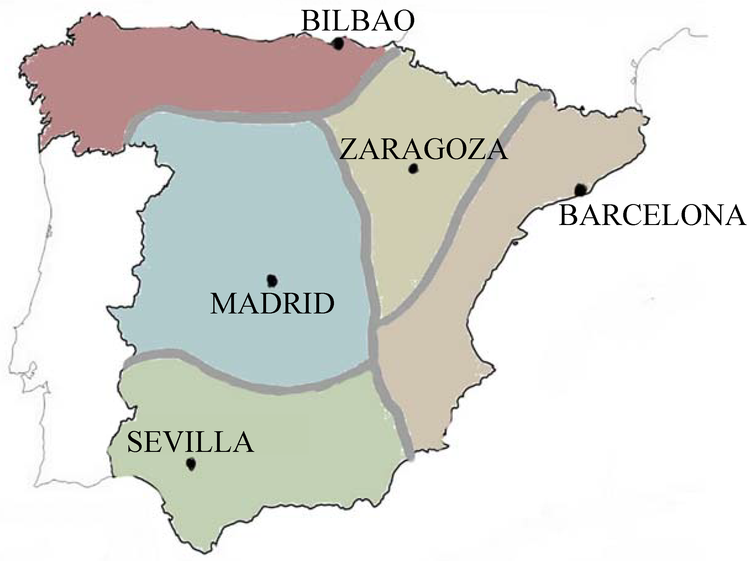
In our case, Spain is a large country with a wide weather diversity. In addition, the population distribution also causes a high variability of power consumption among areas. According to this, the model used at REE includes data from five locations that represent the five weather regions: North-Atlantic (Bilbao), Mediterranean (Barcelona), Upper-Center (Zaragoza), Lower-Center (Madrid) and South (Sevilla). These cities, shown in Figure 2 are the most power demanding areas in each weather region.

The lack of availability of all temperature series affects the accuracy of the system. Both models have been tested by including only one series of data and then adding the rest one at a time. This experiment allows to determine which model can perform best under scarce information and which can benefit the most from a richer dataset.

2.2.3. Temperature Treatment

As it was aforementioned, temperature has a non-linear relation with electricity consumption, as both high and low temperature causes an increase in demand. To illustrate this, Figure 3 shows a plot of the average load on regular days at 18 h against the average temperature of the day. Therefore, in order for the forecasting engine to capture such behavior, it may require a pre-processing of the data.

One common approach to this is using a technique called Heating Degree Days (HDD) and Cooling Degree Days (CDD). This technique linearizes the temperature load relation by defining threshold for high and low temperatures and splitting the series into one that accounts for cold days and another that does for hot days. The CDD and HDD series are described in Equations (3) and (4) and they are further discussed in [34].

$$CD{D}_d=\{\begin{array}{c}{T}_{med,d}-T{H}_{hot}, \mathrm{if} T_{med}>T{H}_{hot} \\ 0, \mathrm{otherwise}\end{array}$$

(3)

$$HD{D}_d=\{\begin{array}{c}T{H}_{cold}-T_{med,d}, \mathrm{if} T_{med}<T{H}_{cold} \\ 0, \mathrm{otherwise}\end{array}$$

(4)

where T_med,d is the average temperature of day d, TH_hot and TH_cold are the thresholds for hot and cold days and CDD_d and HDD_d are the values of each series for day d.

This technique requires the thresholds to be properly tuned to each location’s effect on the load. This optimization process is described in [39] and the optimal threshold for each zone has been calculated. However, the robustness of each model against the variation of these values has been tested by introducing variations of up to 12 degrees on each threshold.

2.2.4. Neural Network Size, Redundancy and Computational Burden

According to the selected topology shown in Figure 1, part of the configuration of the network is the selection of the number of neurons in the hidden layer. The complexity of the network is related to this parameter, as it is associated to its ability to model non-linear behaviors. A network with a low number of neurons in its hidden layer would fail to learn complex, non-linear relations between input and output. On the other hand, the number of neurons increases the computational burden of the training and forecasting process and, therefore it should be minimized if the system is working online and has a response time limit.

In addition, the neural network training algorithm relies on a random initialization of the neurons’ weights. The randomness causes the network’s output to contain a random component. In order to minimize the effect of this randomness, the working model includes a redundant design. Each network is replicated n times to obtain n different outputs for each forecast. The final output is obtained then by discarding the lowest and highest values and averaging the rest. Increasing the number of replicas costs a linear increase of computational burden while it reduces the randomness of the output and reduces the variability of the output, minimizing the maximum error of a forecasted period.

The response time of the system is a critical feature. If the forecast is not produced on time, then the whole effort could be useless. In order to test how the limit of time response affects the models the number of neurons is set from 3 to 20 and the number of redundant networks from 3 to 25. As the neural network model is the one with higher computational burden it is the only one affected by this limitation.

2.2.5. Frequency of Training

As it will be further discussed in Section 3, the load series evolve over time due to changes in factors like economic growth or shifts in consumer behaviors. This causes forecasting models to become obsolete if the data used during training no longer follows the current trends. Therefore, in order to keep up with load shifting behavior, forecasting models need to be frequently retrained with new data.

The training process may have heavy computational requirements that make it unpractical to increase frequency needlessly. Therefore, the period in between trainings is a factor that may alter the accuracy of the model.

In this research, both AR and NN models have been tested with training frequencies of 3, 6, 12 and 24 months. In each of these tests, all sub-models were retrained using the most recent data. In accordance with this, for frequencies higher than 12 months, the simulation period of one year was split into separate blocks as the

Table 1. Training and simulation periods used for testing the effect of training frequency.

Frequency (Months)	Block	Training Period		Simulation Period
		Start	End	Start	End
3	1	1 January 2010	31 December 2016	1 January 2017	31 March 2017
	2	1 April 2010	31 March 2017	1 April 2017	30 June 2017
	3	1 July 2010	30 June 2017	1 July 2017	30 September 2017
	4	1 October 2010	30 September 2017	1 October 2017	31 December 2017
6	1	1 January 2010	31 December 2016	1 January 2017	30 June 2017
	2	1 July 2010	30 June 2017	1 July 2017	31 December 2017
12	1	1 January 2010	31 December 2016	1 January 2017	31 December 2017
24	1	1 January 2009	31 December 2015	1 January 2017	31 December 2017

shows.

To evaluate the results, all blocks from each frequency are added together into a single one-year period and the corresponding Root Mean Square Error (RMSE) is calculated for both AR and NN models.

2.2.6. Number of Auto-Regressive Lags

As it was aforementioned, both models present an auto-regressive component. This part of the model introduces the previous values as a feedback in order to enable to forecasting engine to reduce errors due to unaccounted factors that are persistent in time.

The key parameter to configure this aspect of the models is the number of lags, which represents how many previous values are fed back into the model. Intuitively, the most recent values carry the most information while the further back in time that we reach, the less relevant the data become. In addition, the AR model uses a linear relation to capture the lagged results while the NN model allows non-linearity. Therefore, it is possible that one model is able to use a different amount of lags than the other.

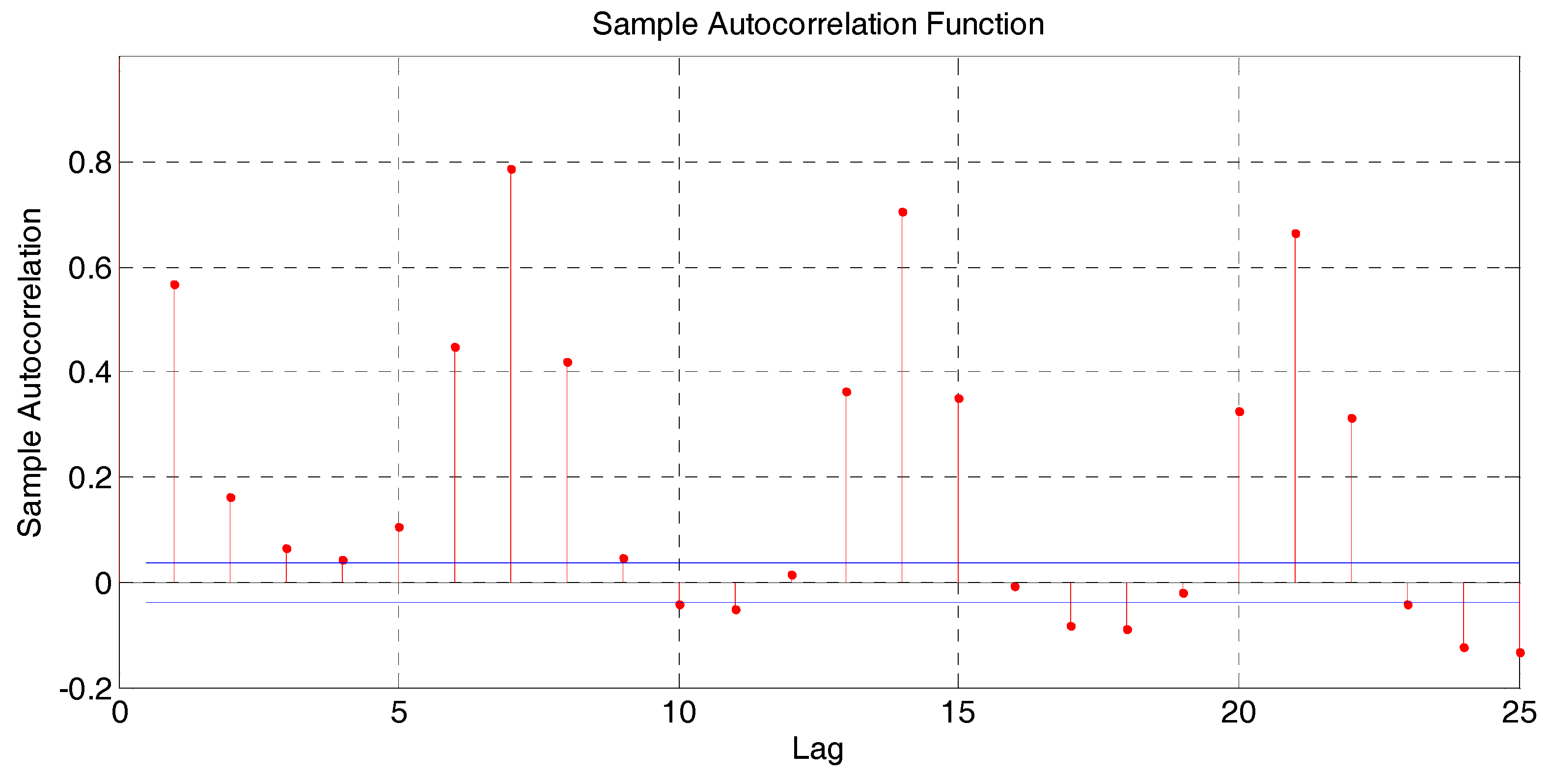
The auto-regressive order of each model has been tested from 0 to 25. The load series is highly self-correlated on lags multiple of seven due to the weekly patterns, as it is shown in Figure 4. Therefore, lags around 7, 14 and 21 were explored. Auto-correlation measures the correlation between y_t and y_t+k, and its calculation is described in [43].

It is worth mentioning that the objective of this paper is not to provide or suggest analytical or statistical methods to determine the order of auto-regressive models like [44,45] but to offer a comparison between AR and NN based models to understand the effect that the auto-regressive order has on the forecasting accuracy.

2.3. Types of Days

Each of the proposed parameters and conditions under which the forecasting models are tested will cause the forecasting accuracy to change over the whole one-year simulating period. This variation, however, may affect some type of days more than other and, therefore, it may seem irrelevant when it is averaged over the whole testing period. In order to avoid this error, it is important to dissect the results and analyze the accuracy of the models on different categories of days to determine which conditions affect which type of days and how they do it.

There are two aspects to classify the days: social character and temperature. The first one considers days as special if they are a holiday, are in between two holidays or weekend, or are affected by Daylight Saving Time or the vacational periods at Christmas or Easter. A more detailed description of the days considered special is found in Section 3.

Temperature is used to classify days as hot and cold. For each category, the top 20 and bottom 20 days from the temperature series are considered. If one of the 20 days is also a special day, then it is discarded as either hot or cold. All days that do not belong to one of the categories (special, hot or cold) are considered as regular days.

3. Data Analysis

It is important to describe the characteristics of the data series relevant to the forecasting process in order to understand the forecasting problem and whether or not its conclusions may apply to a different case:

3.1. Load

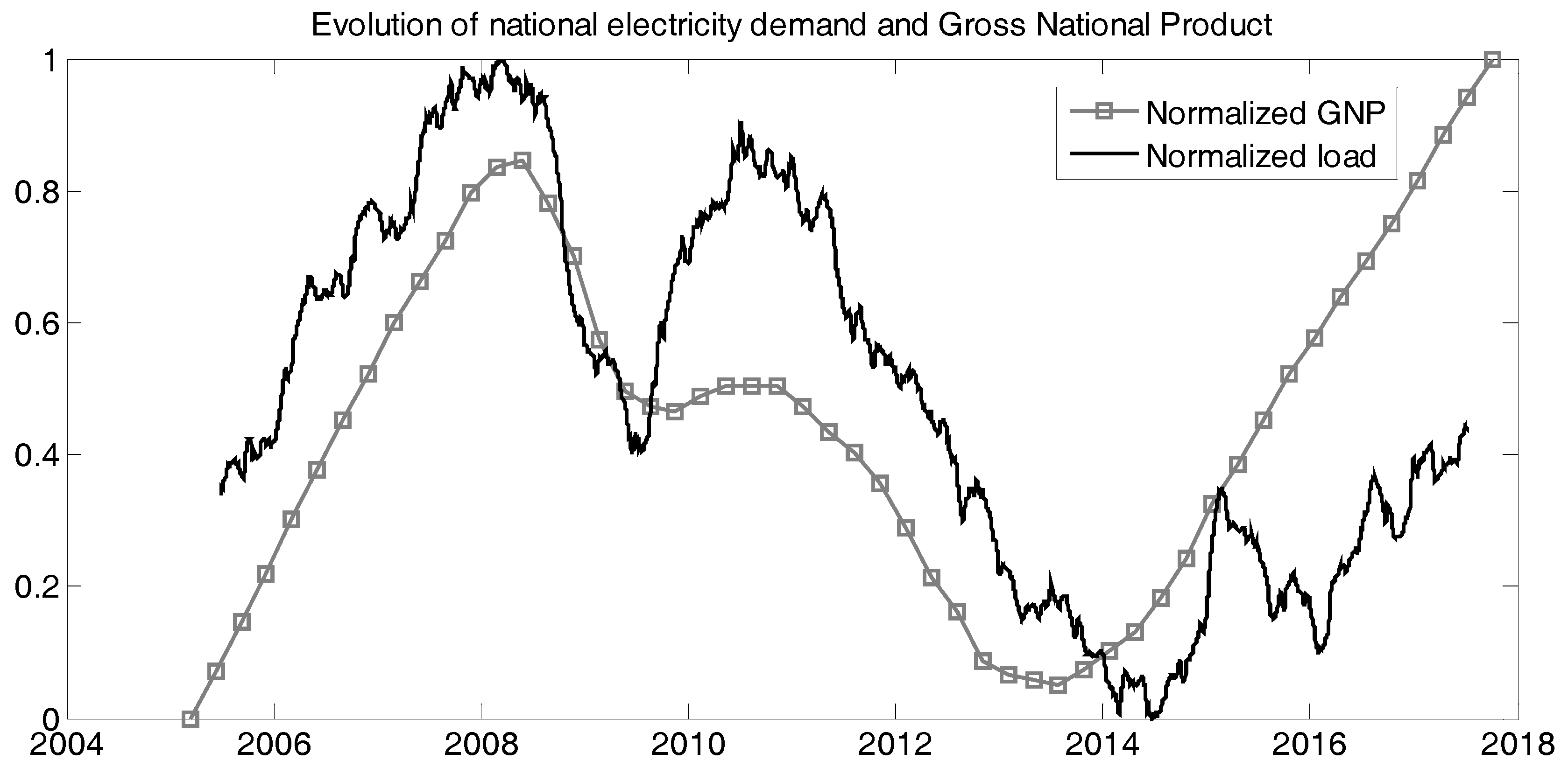
The load data series covers from 2010 to 2017 and it includes hourly values of electricity consumption in the Spanish inland system. The long-term trend of the series shown in Figure 5 is related to economic growth, efficiency improvements and behavioral shifts like the use of AC systems.

On a shorter term scale, the factors driving the load in Spain are temperature and social events and holidays, which are explained in the following subsections.

3.2. Temperature

The temperature data available includes series from 59 stations scattered across the country. Real data of daily maximum and minimum data is collected along with daily forecasts of up to ten days ahead. Therefore, it is possible to simulate real time conditions if forecasts are used instead of real data.

As it was explained before, the national forecast only uses information from five stations selected from the 59 available. This selection is made through an empirical evaluation. In addition, the temperature from up to four previous days is also used in order to capture the dynamics of the temperature-load relation. The non-linearity of the relation is modeled using the CDD and HDD approach already discussed. Figure 6 shows the scatter plot of national load at 18 h on weekday against temperature at the three most relevant locations. The HDD and CDD linearization is also plotted for each location along with the Mean Average Percentage Error (MAPE) between the actual load and the linearized one.

3.3. Calendar

The type of day is determined by the official national calendar published in the Official Gazette [46]. The days are classified into 34 exclusive categories some of which include several days under a general rule: Mondays, Wednesdays, national holidays, Mondays before a holiday… and others for specific and unique days: 1 May, 25 December, 1 January… In addition to the exclusive categories (each day can only be assigned to one of these), there are also 18 modifying categories that may be simultaneously active with an exclusive one. These include regional holidays, days affected by DST… The complete classification can be found in [39].

The relevance of a proper day categorization is shown in Figure 7. The graph represents the average load profiles for 8 December, which is a national holiday, 7 December, before a holiday, and 30 November, regular day 7 days prior to 7 December. The years considered are the ones in which 7 December was not Saturday, Sunday or Monday. Figure 7 also includes the profile for 7 December on a Saturday. The graph shows how depending on the calendar (effects of temperature are averaged out), the profile not only shows variation of up to 20% from a regular weekday to a national holiday but it also shows different profiles in between.

4. Results

The results expressed in this section correspond to the forecasting period of 2017. Each subsection presents the accuracy of both techniques (AR and NN) when the correspondent parameter or external condition changes. In addition, these results have been analyzed under the categories described in Section 2.3.

4.1. Historical Load Availability

The results shown in

Table 2. Forecasting error (RMSE) with training periods from 3 to 7 years.

Type of Day	3-Years		5-Years		7-Years
	AR	NN	AR	NN	AR	NN
Overall	1.50%	2.17%	1.52%	1.72%	1.45%	1.55%
Regular	1.44%	1.96%	1.47%	1.57%	1.40%	1.44%
Special	1.91%	3.62%	1.81%	2.71%	1.81%	2.31%
Hot	1.63%	2.65%	1.53%	2.08%	1.55%	1.93%
Cold	1.61%	2.79%	1.73%	1.81%	1.72%	1.48%

Test conditions: 10 neurons (10N), 10 redundant networks (10RN), 5 temperature locations (5TL), 12 month training freq (12MF), 7 lags for AR and 14 for NN (7/14LAG).

represent the effect of increasing the number of previous years considered in the training of the model from 3 to 7 for both models. The results show a generally more accurate performance by the AR model especially with fewer years of data (1.50% vs. 2.17%). The NN model, however, benefits more from the availability of more data and this difference is reduced to 0.1% when seven years are used. The AR model shows very little improvement from 3 to 7 years while the NN model appears to be able to benefit from even longer training data as its performance on all categories continues to improve from 5 to 7 years (see Figure 8). Unfortunately, the available data base is not yet deep enough to test this.

Regarding the categorized results, regular days obtain almost the same result while in hot and special days the AR outperforms the NN model. However, cold days are clearly forecasted more accurately by the NN model. This could imply that the linear restriction present in the AR model limits its capacity to model the behavior of the load with the data treatment used.

4.2. Temperature Locations

The results for testing the availability of temperature data series from different locations are included in

Table 3. Forecasting error (RMSE) with available temperature location from 1 to 5.

Type of Day	MAD		MAD, BAR		MAD, BAR, VIZ		MAD, BAR, VIZ, SEV		MAD, BAR, VIZ, SEV, ZAR
	AR	NN	AR	NN	AR	NN	AR	NN	AR	NN
Overall	1.63%	1.61%	1.53%	1.59%	1.48%	1.54%	1.46%	1.54%	1.45%	1.55%
Regular	1.59%	1.53%	1.48%	1.50%	1.43%	1.45%	1.41%	1.44%	1.40%	1.44%
Special	1.84%	2.22%	1.86%	2.21%	1.81%	2.15%	1.80%	2.17%	1.81%	2.31%
Hot	1.83%	2.02%	1.63%	1.91%	1.52%	1.84%	1.55%	1.94%	1.55%	1.93%
Cold	2.00%	1.61%	1.81%	1.49%	1.83%	1.47%	1.76%	1.48%	1.72%	1.48%

Test conditions: 7 Years Training (7YT), 10N, 10RN, 12MF, 7/14LAG.

. In addition, Figure 9 shows the evolution of the overall RMSE of both models from having only location to including all five. Locations are included sequentially from most to least relevant.

The NN outperforms the AR model when only one location is available. Both models benefit from having more data series included, but the AR model obtains a more accurate forecast with five locations. In fact, the NN model obtains a larger error with five locations than it does with four. This could imply that the linear restriction on the AR model allows it to correctly include this information in the model. The excessive availability of information, however, seems to increase the risk of NN model overfitting the training data and, therefore, losing forecasting capabilities.

4.3. Temperature Treatment

The preprocessing of the temperature data is a key aspect of the forecasting system. The thresholds need to be properly tuned so that the linearization of the relation is correct. However, these thresholds may shift over time as consumers’ behavior regarding temperature changes. Therefore, robustness to this configuration is also important.

The results were obtained using one location each time and varying HDD and CDD thresholds from 13 to 25 °C.

Table 4. Forecasting error (RMSE) with different HDD threshold adjustment in Barcelona.

Type of Day and Model		HDD Threshold
		13	14	15	16	17	18	19	20	21	22	23	24	25
Overall	AR	2.00%	1.98%	1.96%	1.95%	1.94%	1.92%	1.91%	1.91%	1.91%	1.91%	1.92%	1.93%	1.94%
	NN	1.92%	1.93%	1.93%	1.93%	1.94%	1.92%	1.92%	1.93%	1.92%	1.92%	1.93%	1.93%	1.94%
Hot	AR	2.62%	2.63%	2.63%	2.62%	2.60%	2.58%	2.55%	2.53%	2.50%	2.48%	2.46%	2.43%	2.45%
	NN	2.54%	2.55%	2.55%	2.53%	2.56%	2.54%	2.55%	2.54%	2.52%	2.51%	2.51%	2.46%	2.47%
Cold	AR	2.16%	2.11%	2.07%	2.03%	2.00%	1.99%	1.99%	1.99%	1.99%	2.00%	2.01%	2.02%	2.02%
	NN	1.65%	1.67%	1.69%	1.71%	1.71%	1.68%	1.71%	1.68%	1.72%	1.67%	1.71%	1.69%	1.69%

shows the overall results for shifting the HDD threshold for Barcelona along with the hot and cold categories as the special days are not relevant to this test.

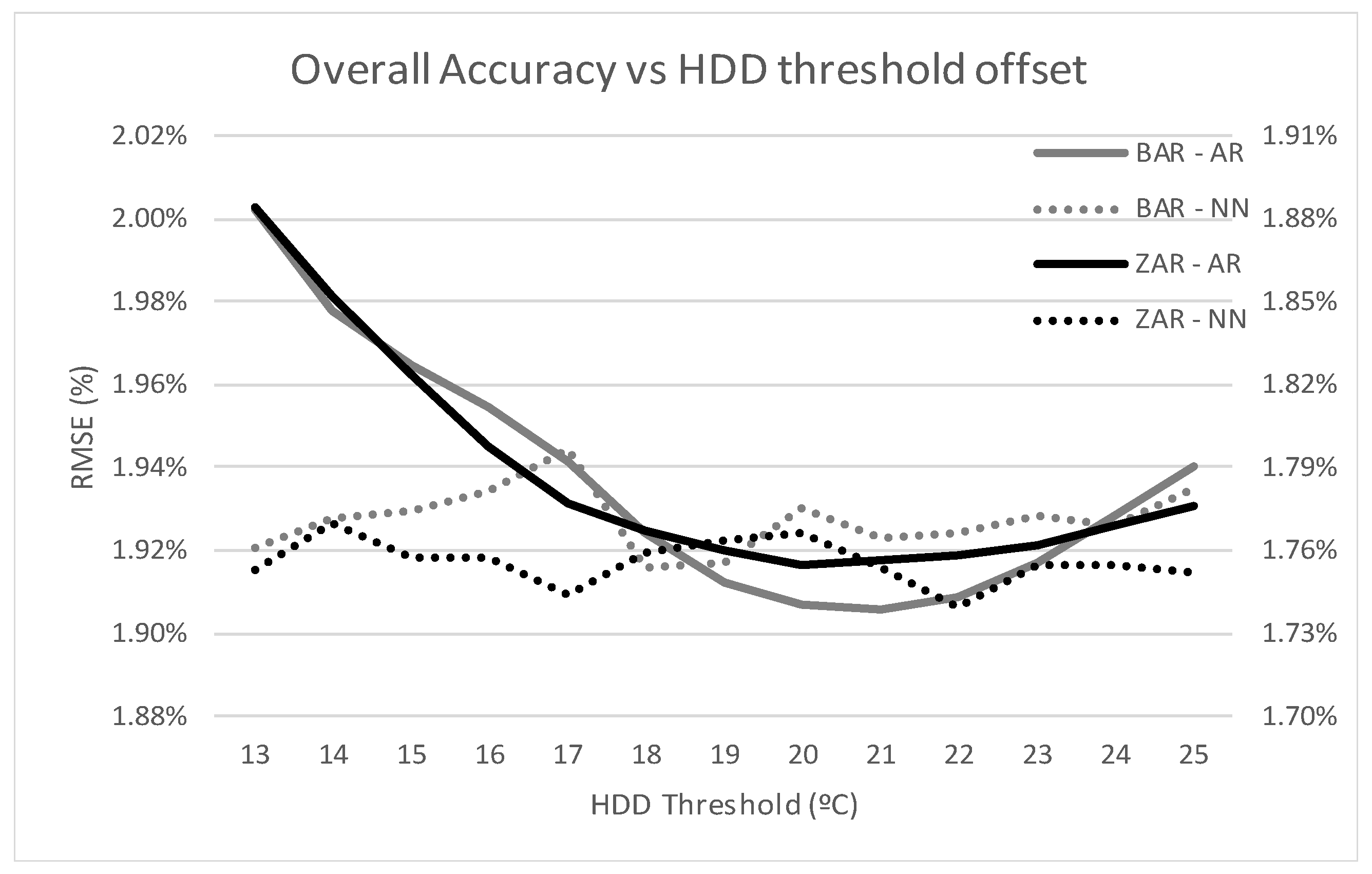
The effect of adjusting the threshold is more clearly shown in Figure 10, in which forecasting accuracy of both models using temperature from Zaragoza and Barcelona is plotted. The graph shows how the NN is much less dependent on the chosen threshold while the AR performance is clearly thrown off by a misadjusted threshold.

4.4. Number of Neurons

The number of neurons in the hidden layer affects both computational burden and the NN’s performance. Therefore, both aspects are reported as results on this test.

Table 5. Forecasting error (RMSE) and execution time with different number of neurons.

Type of Day	Number of Neurons
	3	4	5	10	15	20
Overall	1.56%	1.55%	1.56%	1.55%	1.58%	1.62%
Regular	1.49%	1.46%	1.45%	1.44%	1.46%	1.50%
Special	2.00%	2.10%	2.28%	2.31%	2.36%	2.46%
Hot	2.00%	1.93%	1.95%	1.93%	2.00%	2.04%
Cold	1.55%	1.45%	1.51%	1.48%	1.51%	1.58%
Time (s)	1.610	1.615	1.620	1.630	1.639	1.643

Test conditions: 7YT, 10RN, 5TL, 12MF, 7/14LAG.

shows the accuracy of the neural network as the number of neurons is increased. In addition, the forecasting time for a single 24-h profile is included. It is worth noticing that the rest of forecasting processes like data access or treatment also consume time and, therefore, the reported time is not the only concern in order to obtain a timely forecast.

Figure 11 shows the evolution of accuracy and simulation time against the number of neurons in the hidden layer. It can be seen that the execution time is almost constant and therefore the number of neurons is not an issue regarding computational burden. In addition, accuracy on regular days does not improve with more complex networks. Special days, however, show a deterioration as the number of neurons increases. A possible explanation to this is that a more complex network is able to overfit the training data and lose generality. This is especially obvious on the special-day category due to the scarcity of data.

4.5. Redundancy of Neural Networks

The use of a redundant number of NN reduces the model’s dependency of random initial conditions. Furthermore, eliminating extreme values also reduces the overall error.

Table 6. Forecasting error (RMSE) and execution time with different redundant networks.

Type of Day	Number of Networks
	3	5	10	11	12	14	15	16	20	25
Overall	1.67%	1.62%	1.55%	1.56%	1.54%	1.54%	1.54%	1.55%	1.55%	1.56%
Regular	1.55%	1.51%	1.46%	1.48%	1.46%	1.45%	1.46%	1.46%	1.45%	1.46%
Special	2.51%	2.30%	2.10%	2.08%	2.08%	2.11%	2.12%	2.13%	2.18%	2.22%
Hot	2.02%	1.97%	1.93%	1.98%	1.92%	1.94%	1.92%	1.93%	1.92%	1.94%
Cold	1.54%	1.57%	1.45%	1.43%	1.45%	1.43%	1.44%	1.46%	1.47%	1.44%
Time (s)	0.839	1.09	1.686	1.746	1.868	2.039	2.228	2.333	2.713	3.363

Test conditions: 7YT, 4N, 5TL, 12MF, 7/14LAG.

shows the results of using from 3 to 25 redundant networks for the NN model.

There is an improvement using up to 10 redundant networks. However, there is not significant error reduction from 10 to 25 networks. The execution time shows an increase, although for the optimum amount of 10 networks the computational burden is still manageable. As a reference, we have used the execution time for the AR model, which is 0.835 s. In addition, in Figure 12 it can be seen that the type of days that benefit the most from increasing number of networks from 3 to 10 are special days. Again, this is probably due to the higher variability in the output from different networks for this scarcer type of days.

4.6. Frequency of Training

The results from

Table 7. Forecasting error (RMSE) with different training frequency.

Type of Day	3 Months		6 Months		12 Months		24 Months
	AR	NN	AR	NN	AR	NN	AR	NN
Overall	1.44%	1.54%	1.44%	1.56%	1.45%	1.55%	1.78%	2.07%
Regular	1.39%	1.45%	1.40%	1.47%	1.40%	1.46%	1.74%	2.01%
Special	1.78%	2.09%	1.79%	2.10%	1.81%	2.10%	2.13%	2.35%
Hot	1.57%	1.96%	1.57%	1.97%	1.55%	1.93%	2.26%	3.11%
Cold	1.70%	1.45%	1.69%	1.46%	1.72%	1.45%	1.96%	1.96%

Test conditions: 7YT, 4N, 10RN, 5TL, 7/14LAG.

show the performance of both models when the training period is changed from 3 months to 24 months. The testing period remains the same as described in Table 1, but the data used to train the model that forecasted each block changes. There appear to be no significant improvement from retraining the models more frequently than annually, as seen on Figure 13. However, a training period longer than a year seems to cause an increase in the forecasting error. Both models are affected very similarly by this parameter, with an increase in the error of about 23% for both models when increasing the time in between trainings from 12 to 24 months.

4.7. Number of Lags

The number of lags in each model is changed from 0 to 25 in order to expose how this parameter affects the accuracy of each model. The results are categorized by type of day on

Table 8. Forecasting error (RMSE) with different lagged feedback.

LAG	Overall		Regular		Special		Hot		Cold
	AR	NN	AR	NN	AR	NN	AR	NN	AR	NN
0	1.80%	1.73%	1.76%	1.64%	2.08%	2.31%	1.94%	1.89%	2.00%	1.57%
1	1.73%	1.65%	1.68%	1.55%	2.04%	2.34%	1.86%	1.81%	1.85%	1.47%
3	1.64%	1.61%	1.59%	1.49%	1.96%	2.36%	1.81%	1.82%	1.87%	1.53%
5	1.62%	1.57%	1.57%	1.48%	1.95%	2.16%	1.81%	1.91%	1.86%	1.44%
6	1.56%	1.56%	1.51%	1.47%	1.89%	2.11%	1.75%	1.91%	1.81%	1.41%
7	1.45%	1.56%	1.40%	1.47%	1.81%	2.14%	1.55%	1.89%	1.72%	1.47%
8	1.45%	1.55%	1.39%	1.46%	1.81%	2.15%	1.55%	1.90%	1.72%	1.45%
13	1.45%	1.57%	1.39%	1.47%	1.84%	2.16%	1.52%	1.97%	1.72%	1.45%
14	1.43%	1.55%	1.37%	1.46%	1.83%	2.10%	1.51%	1.93%	1.71%	1.45%
15	1.43%	1.57%	1.37%	1.48%	1.83%	2.15%	1.51%	1.92%	1.71%	1.50%
20	1.43%	1.58%	1.37%	1.48%	1.83%	2.21%	1.52%	1.95%	1.70%	1.48%
21	1.42%	1.56%	1.35%	1.48%	1.83%	2.08%	1.49%	1.91%	1.68%	1.48%
22	1.42%	1.54%	1.35%	1.46%	1.83%	2.03%	1.50%	1.92%	1.68%	1.45%
24	1.42%	1.58%	1.36%	1.48%	1.84%	2.17%	1.50%	1.93%	1.68%	1.47%
25	1.42%	1.59%	1.35%	1.49%	1.84%	2.25%	1.50%	1.92%	1.68%	1.49%

Test conditions: 7YT, 4N, 10RN, 5TL, 12MF.

. The AR model obtains a less accurate forecast than the NN when the lags are below 7 days. However, the results beyond this threshold benefit the AR model clearly. The AR model seems to continue its improvement up to lag number 21 (three weeks) but the NN reaches a plateau at lag 7. Once again, the NN model performs more accurately when little information (in this case lags) is available but it is outperformed by the AR model when the limitation is lifted. Figure 14 represents the overall accuracy of both models as the number of lags is increased. It is worth noticing how the AR model improves specially at lags 7, 14 and 21.

4.8. Overall Results

The previous subsections show how there is not a single solution for the load-forecasting problem. The conditions under which the forecast is done due to availability or data or time constraints affect the accuracy of each technique differently and, therefore, these conditions need to be taken into consideration when designing a forecasting system. As a general result, the AR model appears to be slightly more accurate but requires a finer tuning when treating the temperature data and requires a larger amount of temperature data sources.

5. Conclusions

Many different short-term load forecasting models have been proposed in the recent years. However, it is difficult to compare the accuracy or the general performance of each model when each one is tested under different conditions, testing periods and databases. The goal of this paper is to provide a series of comparisons between two of the most used forecasting engines: auto-regressive models and neural networks. The starting point is a forecasting system currently in use by REE that includes both techniques. Several tests have been run in order to determine the conditions under which each model performs best.

The results show that both models obtain very similar accuracy and, therefore both of them should remain in use. The AR model obtained a better overall result under the best possible condition but the NN model was superior when fewer temperature locations are available, the treatment of the temperature data is not properly adjusted or the feedback is limited to less than 7 lagged days. The AR showed higher accuracy when historical data is limited to less than 7 years. Both models have the same needs in terms of training frequency: a one-year period in between trainings is sufficient.

Regarding computational burden, the AR model is less computationally intense than the NN. However, the optimum configuration found at 4 neurons in the hidden layer and 10 redundant networks only costs twice as much as the AR model. Therefore, neither model has a definite advantage on this front.

To sum up, this paper enables the researcher to establish a set of rules to guide them in the process of selecting or designing a forecasting system. The results of this research offer very practical information that responds to actual empirical implementations of the system rather than to theoretical experiments. Further research in this area should include the analysis of different databases from other systems. The use of information from other systems would help determine if the conclusions drawn are general or database specific, in which case, studying the specificities of each database and determining why they behave differently would also be of value to the field.

References

- Hippert, H.S.; Pedreira, C.E.; Souza, R.C. Neural networks for short-term load forecasting: A review and evaluation. IEEE Trans. Power Syst. 2001, 16, 44–55. [Google Scholar] [CrossRef]
- Hong, T.; Fan, S. Probabilistic electric load forecasting: A tutorial review. Int. J. Forecast. 2016, 32, 914–938. [Google Scholar] [CrossRef]
- Kuster, C.; Rezgui, Y.; Mourshed, M. Electrical load forecasting models: A critical systematic review. Sustain. Cities Soc. 2017, 35, 257–270. [Google Scholar] [CrossRef] [Green Version]
- Papalexopoulos, A.D.; Hesterberg, T.C. A regression-based approach to short-term system load forecasting. IEEE Trans. Power Syst. 1990, 5, 1535–1547. [Google Scholar] [CrossRef]
- Charlton, N.; Singleton, C. A refined parametric model for short term load forecasting. Int. J. Forecast. 2014, 30, 364–368. [Google Scholar] [CrossRef]
- Wang, P.; Liu, B.; Hong, T. Electric load forecasting with recency effect: A big data approach. Int. J. Forecast. 2016, 32, 585–597. [Google Scholar] [CrossRef]
- Hagan, M.T.; Behr, S.M. The Time Series Approach to Short Term Load Forecasting. IEEE Trans. Power Syst. 1987, 2, 785–791. [Google Scholar] [CrossRef]
- Amjady, N. Short-term hourly load forecasting using time-series modeling with peak load estimation capability. IEEE Trans. Power Syst. 2001, 16, 498–505. [Google Scholar] [CrossRef]
- Amini, M.H.; Kargarian, A.; Karabasoglu, O. ARIMA-based decoupled time series forecasting of electric vehicle charging demand for stochastic power system operation. Electr. Power Syst. Res. 2016, 140, 378–390. [Google Scholar] [CrossRef]
- Boroojeni, K.G.; Amini, M.H.; Bahrami, S.; Iyengar, S.S.; Sarwat, A.I.; Karabasoglu, O. A novel multi-time-scale modeling for electric power demand forecasting: From short-term to medium-term horizon. Electr. Power Syst. Res. 2017, 142, 58–73. [Google Scholar] [CrossRef]
- Taylor, J.W. Short-Term Load Forecasting with Exponentially Weighted Methods. IEEE Trans. Power Syst. 2012, 27, 458–464. [Google Scholar] [CrossRef]
- Mandal, P.; Senjyu, T.; Urasaki, N.; Funabashi, T. A neural network based several-hour-ahead electric load forecasting using similar days approach. Int. J. Electr. Power Energy Syst. 2006, 28, 367–373. [Google Scholar] [CrossRef]
- Zhang, Y.; Zhou, Q.; Sun, C.; Lei, S.; Liu, Y.; Song, Y. RBF Neural Network and ANFIS-Based Short-Term Load Forecasting Approach in Real-Time Price Environment. IEEE Trans. Power Syst. 2008, 23, 853–858. [Google Scholar] [CrossRef]
- Kalaitzakis, K.; Stavrakakis, G.S.; Anagnostakis, E.M. Short-term load forecasting based on artificial neural networks parallel implementation. Electr. Power Syst. Res. 2002, 63, 185–196. [Google Scholar] [CrossRef]
- Liao, G.-C.; Tsao, T.-P. Application of a fuzzy neural network combined with a chaos genetic algorithm and simulated annealing to short-term load forecasting. IEEE Trans. Evol. Comput. 2006, 10, 330–340. [Google Scholar] [CrossRef]
- López, M.; Valero, S.; Senabre, C.; Aparicio, J.; Gabaldon, A. Application of SOM neural networks to short-term load forecasting: The Spanish electricity market case study. Electr. Power Syst. Res. 2012, 91, 18–27. [Google Scholar] [CrossRef]
- Hinojosa, V.H.; Hoese, A. Short-Term Load Forecasting Using Fuzzy Inductive Reasoning and Evolutionary Algorithms. IEEE Trans. Power Syst. 2010, 25, 565–574. [Google Scholar] [CrossRef]
- Srinivasan, D.; Chang, C.S.; Liew, A.C. Demand forecasting using fuzzy neural computation, with special emphasis on weekend and public holiday forecasting. IEEE Trans. Power Syst. 1995, 10, 1897–1903. [Google Scholar] [CrossRef]
- Kim, K.-H.; Youn, H.-S.; Kang, Y.-C. Short-term load forecasting for special days in anomalous load conditions using neural networks and fuzzy inference method. IEEE Trans. Power Syst. 2000, 15, 559–565. [Google Scholar]
- Song, K.-B.; Baek, Y.-S.; Hong, D.H.; Jang, G. Short-term load forecasting for the holidays using fuzzy linear regression method. IEEE Trans. Power Syst. 2005, 20, 96–101. [Google Scholar] [CrossRef]
- Chen, Y.; Yang, Y.; Liu, C.; Li, C.; Li, L. A hybrid application algorithm based on the support vector machine and artificial intelligence: An example of electric load forecasting. Appl. Math. Model. 2015, 39, 2617–2632. [Google Scholar] [CrossRef]
- Wang, J.; Jin, S.; Qin, S.; Jiang, H. Swarm Intelligence-based hybrid models for short-term power load prediction. Math. Probl. Eng. 2014, 2014, 17. [Google Scholar] [CrossRef]
- Bashir, Z.A.; El-Hawary, M.E. Applying wavelets to short-term load forecasting using pso-based neural networks. IEEE Trans. Power Syst. 2009, 24, 20–27. [Google Scholar] [CrossRef]
- Amjady, N.; Keynia, F. Short-term load forecasting of power systems by combination of wavelet transform and neuro-evolutionary algorithm. Energy 2009, 34, 46–57. [Google Scholar] [CrossRef]
- Ho, K.-L.; Hsu, Y.-Y.; Chen, C.-F.; Lee, T.-E.; Liang, C.-C.; Lai, T.-S.; Chen, K.-K. Short term load forecasting of Taiwan power system using a knowledge-based expert system. IEEE Trans. Power Syst. 1990, 5, 1214–1221. [Google Scholar]
- Huang, C.-M.; Huang, C.-J.; Wang, M.-L. A particle swarm optimization to identifying the ARMAX model for short-term load forecasting. IEEE Trans. Power Syst. 2005, 20, 1126–1133. [Google Scholar] [CrossRef]
- Niu, D.; Xing, M. Research on neural networks based on culture particle swarm optimization and its application in power load forecasting. In Proceedings of the Third International Conference on Natural Computation (ICNC 2007), Haikou, China, 24–27 August 2007; Volume 1, pp. 270–274. [Google Scholar]
- Gajowniczek, K.; Ząbkowski, T. Electricity forecasting on the individual household level enhanced based on activity patterns. PLoS ONE 2017, 12, e0174098. [Google Scholar] [CrossRef] [PubMed]
- Singh, S.; Yassine, A. Big data mining of energy time series for behavioral analytics and energy consumption forecasting. Energies 2018, 11, 452. [Google Scholar] [CrossRef]
- López, M.; Valero, S.; Senabre, C.; Aparicio, J.; Gabaldon, A. Standardization of short-term load forecasting models. In Proceedings of the 2012 9th International Conference on the European Energy Market, Florence, Italy, 10–12 May 2012; pp. 1–7. [Google Scholar]
- Kim, C.; Yu, I.; Song, Y.H. Kohonen neural network and wavelet transform based approach to short-term load forecasting. Electr. Power Syst. Res. 2002, 63, 169–176. [Google Scholar] [CrossRef]
- Chen, Y.; Luh, P.B.; Rourke, S.J. Short-term load forecasting: Similar day-based wavelet neural networks. In Proceedings of the 2008 7th World Congress on Intelligent Control and Automation, Chongqing, China, 25–27 June 2008; pp. 3353–3358. [Google Scholar]
- López, M.; Valero, S.; Senabre, C.; Gabaldón, A. Analysis of the influence of meteorological variables on real-time Short-Term Load Forecasting in Balearic Islands. In Proceedings of the 2017 11th IEEE International Conference on Compatibility, Power Electronics and Power Engineering (CPE-POWERENG), Cadiz, Spain, 4–6 April 2017; pp. 10–15. [Google Scholar]
- Cancelo, J.R.; Espasa, A.; Grafe, R. Forecasting the electricity load from one day to one week ahead for the Spanish system operator. Int. J. Forecast. 2008, 24, 588–602. [Google Scholar] [CrossRef] [Green Version]
- Lamedica, R.; Prudenzi, A.; Sforna, M.; Caciotta, M.; Cencellli, V.O. A neural network based technique for short-term forecasting of anomalous load periods. IEEE Trans. Power Syst. 1996, 11, 1749–1756. [Google Scholar] [CrossRef]
- Arora, S.; Taylor, J.W. Short-term forecasting of anomalous load using rule-based triple seasonal methods. IEEE Trans. Power Syst. 2013, 28, 3235–3242. [Google Scholar] [CrossRef]
- Khotanzad, A.; Afkhami-Rohani, R.; Maratukulam, D. ANNSTLF-artificial neural network short-term load forecaster generation three. IEEE Trans. Power Syst. 1998, 13, 1413–1422. [Google Scholar] [CrossRef]
- Fan, S.; Methaprayoon, K.; Lee, W.-J. Multiregion load forecasting for system with large geographical area. IEEE Trans. Ind. Appl. 2009, 45, 1452–1459. [Google Scholar] [CrossRef]
- López, M.; Valero, S.; Rodriguez, A.; Veiras, I.; Senabre, C. New online load forecasting system for the Spanish transport system operator. Electr. Power Syst. Res. 2018, 154, 401–412. [Google Scholar] [CrossRef]
- Mares, J.J.; Mercado, K.D.; Quintero M., C.G. A Methodology for short-term load forecasting. IEEE Lat. Am. Trans. 2017, 15, 400–407. [Google Scholar] [CrossRef]
- Almeshaiei, E.; Soltan, H. A methodology for electric power load forecasting. Alex. Eng. J. 2011, 50, 137–144. [Google Scholar] [CrossRef]
- García, M.L.; Valero, S.; Senabre, C.; Marín, A.G. Short-term predictability of load series: characterization of load data bases. IEEE Trans. Power Syst. 2013, 28, 2466–2474. [Google Scholar] [CrossRef]
- Box, G.E.P.; Jenkins, G.M.; Reinsel, G.C.; Ljung, G.M. Time Series Analysis: Forecasting and Control, 5th ed.; John Wiley & Sons, Inc.: Hoboken, NJ, USA, 2016. [Google Scholar]
- Akaike, H. Statistical predictor identification. Ann. Inst. Stat. Math. 1970, 22, 203–217. [Google Scholar] [CrossRef]
- Akaike, H. Information theory and an extension of the maximum likelihood principle. In Proceedings of the Second International Symposium on Information Theory, Tsahkadsor, Armenia, 2–8 September 1971; Petrov, B.N., Caski, F., Eds.; Akadémiai Kiado: Budapest, Hungary; pp. 267–281. [Google Scholar]
- Gobierno de España. Boletín Oficial del Estado. Available online: www.boe.es (accessed on 10 April 2018).
Figure 1.
Schematic view of the NARX system as shown on a Matlab Mathworks visualization.
Figure 2.
Location of the five temperature series and distribution of the weather regions in Spain.
Figure 3.
Scatter plot of national load at 18 h against the daily average temperature in Madrid.
Figure 4.
Sample autocorrelation function for National load at 18 h.
Figure 5.
Evolution of 52 weeks moving average load and Gross National Product. Both series are normalized [0, 1].
Figure 6.
Scatter plot of national load and its linearization against temperature at Madrid, Barcelona and Sevilla.
Figure 7.
Different average profiles for national holidays, normal days, Saturdays and adjacent to holiday.
Figure 8.
Overall forecasting error (RMSE) with training periods from 3 to 7 years.
Figure 9.
Overall forecasting error (RMSE) with available temperature location from 1 to 5.
Figure 10.
Overall forecasting error (RMSE) with different HDD threshold adjustment in Barcelona and Zaragoza.
Figure 11.
Overall forecasting error (RMSE) and execution time with different number of neurons.
Figure 12.
Overall forecasting error (RMSE) and execution time with different redundant networks.
Figure 13.
Forecasting error (RMSE) for AR and NN models with training frequency from 3 to 24 months.
Figure 14.
Overall forecasting error (RMSE) with different lagged feedback.