Full-Speed Range Encoderless Control for Salient-Pole PMSM with a Novel Full-Order SMO


1
The School of Automation, Northwestern Polytechnical University, Xi’an 710072, China
2
Quanzhou Institute of Equipment Manufacturing, Haixi Institutes, Chinese Academy of Sciences, Jinjiang 362200, China
*
Author to whom correspondence should be addressed.
Energies 2018, 11(9), 2423; https://doi.org/10.3390/en11092423
Submission received: 15 August 2018
/
Revised: 29 August 2018
/
Accepted: 30 August 2018
/
Published: 13 September 2018
(This article belongs to the Special Issue Control and Nonlinear Dynamics on Energy Conversion Systems)
Abstract
:For salient-pole permanent magnet synchronous motor (PMSM), the amplitude of extended back electromotive force (EEMF) is determined by rotor speed, stator current and its derivative value. Theoretically, even at extremely low speed, the back EEMF can be detected if the current in q-axis is changing. However, it is difficult to detect the EEMF precisely due to the current at low speed. In this paper, novel full-order multi-input and multi-output discrete-time sliding mode observer (SMO) is built to detect the rotor position. With the proposed rotor position estimation technique, the motor can start up from standstill and reverse between positive and negative directions without a position sensor. The proposed method was evaluated by experiment.
1. Introduction
Permanent magnet synchronous motor (PMSM) has many benefits, such as high efficiency, high power density, and good dynamic performance, which has been widely used in various kinds of industrial and domestic applications [1,2].
As is well known, rotor position is required in high-performance control of PMSM, which is usually obtained by using an external dedicated sensor. However, the position sensor may increase cost, weight, volume, and complexity; reduce reliability; and restrict the application area [3,4].
To detect the rotor position information directly from the model of PMSM, various kinds of strategies have been proposed up to date, such as voltage model based methods [5,6], Kalman filter based methods [7,8], and state observers based methods [9,10]. Among them, sliding mode observer (SMO) is a very promising option [11,12,13].
The SMO-based rotor position estimation algorithm of salient-pole PMSM is more complicated than that of non-salient pole PMSM [14]. In coordinate system, the state equations of salient-pole PMSM are coupled with each other. The amplitude of the extended back electromotive force (EEMF) is determined by rotor speed, stator current and its derivative value. It is a challenge to estimate the EEMF accurately [12,13].
To obtain the rotor position of salient-pole PMSM, some SMO-based methods have been proposed. To facilitate digital control applications, a discrete-time SMO is constructed in [11], and a kind of position extraction algorithm is proposed to mitigate the oscillations. In [14], a rotor position estimation method based on extended flux model is proposed, while a discrete-time SMO and a position compensator are designed. A full-order discrete-time SMO-based position sensorless control method is introduced in [15], where the modeling uncertainties and external disturbances are considered.
However, in these studies, two single input and single output (SISO) SMO are built in -axis and -axis, respectively, while the effect of coupling is neglected. A signum function or a sigmoid function is used as switching function, which cannot guarantee the convergence in the boundary layer [16]. During load (torque and/or speed) variations, it is a challenge to estimate the EEMF accurately [13]. Due to unwanted chattering, a filter is required to achieve desired back EEMF signal, which may cause phase shift and estimation error in the rotor position.
In this paper, an alternative rotor position estimation strategy for salient-pole PMSM is proposed. To improve the estimation results, the transient state of back EEMF is considered [17]. A fourth-order state equation of salient-pole PMSM in coordinate system is established; the state vector consists of currents and back EEMF. As the state vector is four-dimensional and input vector is two-dimensional, a novel multiple input and multiple output (MIMO) sliding mode observer is built for the system. To facilitate digital control applications, the sliding mode observer is studied in the discrete-time field. Pole placement technique [18,19] is used to design the switching surface; desired dynamic characteristics can be achieved through eigenvalue placement. To force the state trajectories reach and subsequently remain on the eventual sliding surface with a good movement quality, free hierarchical law is adopted as switching scheme, and discretized reaching law [20] is used to design the quasi-sliding mode and reaching process. Reaching law approach has many merits, such as guaranteeing robustness, reducing chattering, and revealing the motion mechanism of the system [21].
This paper is organized as follows: the SMO-based position sensorless control strategies for salient-pole PMSM are introduced in Section 1. In Section 2, a full-order state equation of salient-pole PMSM is built. In Section 3, a full-order SMO is proposed to detect the back EEMF and rotor position. In Section 4, the experimental results of the proposed position sensorless control are given. The paper is concluded in Section 5.
2. Full-Order State Equation of Salient-Pole PMSM
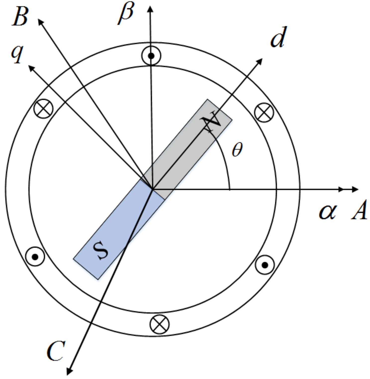
The model of salient-pole PMSM is shown in Figure 1. A, B and C are the three phase windings, represents the stationary reference frame, and means the rotating reference frame.
The motor equation in coordinate frame is expressed as Equation (1) [11].
where P is a derivative operator; is stator resistance; is electrical rotor speed; is electrical rotor angle; is PM flux linkage; are stator inductances; are stator voltages; and are stator currents.
To facilitate the rotor position estimation, inverse Park transformation is used to transform Equation (1) into coordinate frame, as shown in Equation (2).
As is shown in Equation (2), the state equations in -axis and -axis couples with each other. The second term in the right side of Equation (2) is the EEMF; the amplitude of the EEMF is determined by rotor speed, stator current and its derivative value.
The differential of exists in the EEMF. Even the motor is standstill, only if the current changes, the EEMF is not zero. This property is useful for the motor to start up from zero speed and reverse from one direction to the other.
Let denotes the term , then the current model of PMSM is shown as Equation (3).
and in Equation (3) are EEMF, which can be expressed as Equation (4). In conventional second-order SMO-based encoderless control methods, the derivatives of the EMF terms are assumed to be zero (), so the dynamic performance is limited [17,22].
3. Full-Order Sliding Mode Observer Design
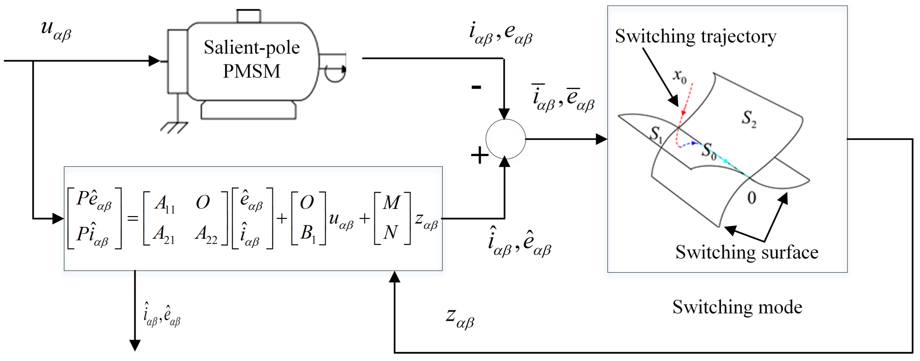
Based on motor state Equation (6), estimated state equation is shown in Equation (7).
where are estimated currents; are estimated EEMF; and are inputs of the estimator, ; ; ; and .
Subtracting Equation (6) from Equation (7), estimation errors are shown in Equation (8).
where and .
Equation (8) is a Multi-Input and Multi-Output (MIMO) system, which can be expressed as Equation (9).
where is a state vector, and is a input vector.
A linear transformation shown as Equation (10) is used to transform Equation (9) into a regular form that has reduced-order, simpler computation, and equivalent dynamics [24].
After transformation, the regular form of the sliding mode observer is shown as Equation (11).
where,
To facilitate digital processor applications, the SMO is studied in discrete-time field. The discrete-time form of the SMO in Equation (11) is expressed as Equation (12).
For the Multiple Input and Multiple Output (MIMO) system, a SMO is designed to estimate the currents and back EEMF in -axis and -axis. The scheme is shown as Figure 2.
The design of the sliding mode control involves two parts: switching surfaces and switching trajectory, as shown in Figure 2. The switching surfaces are designed to ensure the system has desired dynamic characteristics. System state trajectories should reach and remain on the eventual switching surface [19,21].
The dynamics of the system only depends on switching surfaces and is not influenced by system structure and parameter uncertainties [13].
Linear switching surfaces are used in the variable structure control. There are two inputs, so two switching surfaces are designed, which are shown as and in Figure 2.
where ,
The eventual switching surface is , which is shown as Equation (14).
When the sliding mode is enforced in the switching surface, the system’s dynamic characteristics are determined by sliding eigenvalues [19].
In the following, the matrix is expressed as , and are unknown.
As the design of switching surface is not affected by , it can take any arbitrary value [18,19]. To simplify the switching function, is set as a unit matrix .
Equation (12) can be expressed as Equation (15), and the switching function Equation (13) can be expressed as Equation (16).
When the switching trajectory arrives at the switching surface, . Substituting into Equation (18):
Assume the desired poles of the system are and .
Matrix F can be calculated based on Equation (21), and can be obtained according to F and Equation (20). The switching functions are achieved by substituting and into Equation (13).
In this control system, there are three switching surfaces . Free-order switching scheme is adopted, as shown in Figure 2.
Discrete-time reaching law is used to design the sliding mode trajectory, which is shown as Equation (22).
where and are diagonal matrices.
Substituting Equation (24) into Equation (12), the sliding mode trajectory is shown as Equation (25).
Substituting Equation (24) into the discrete-time form of Equation (7), state variables of the system, including currents and EEMF signals , can be achieved.
4. Experimental Results
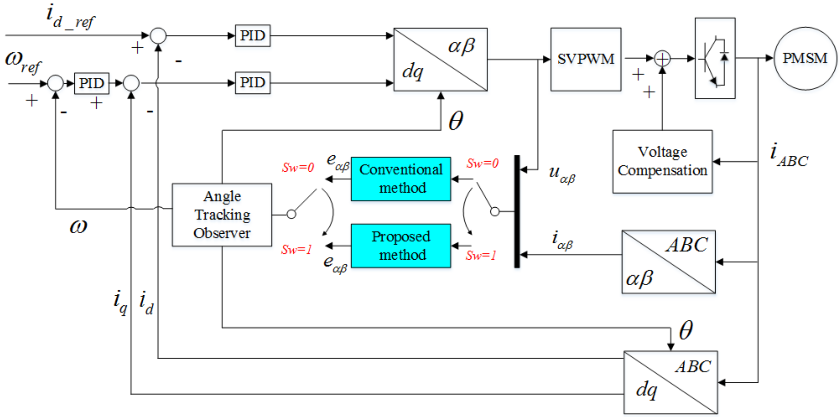
The proposed encoderless method is shown as Figure 4. A conventional full-order discrete-time SMO-based position sensorless control method [15] and the proposed method are compared under the same condition. When , the proposed method is used, otherwise the conventional method is used. The comparison includes computation time, speed variation and torque variation. To show the effectiveness of the proposed method in low speed range, speed reversal experiment and startup experiment are implemented.
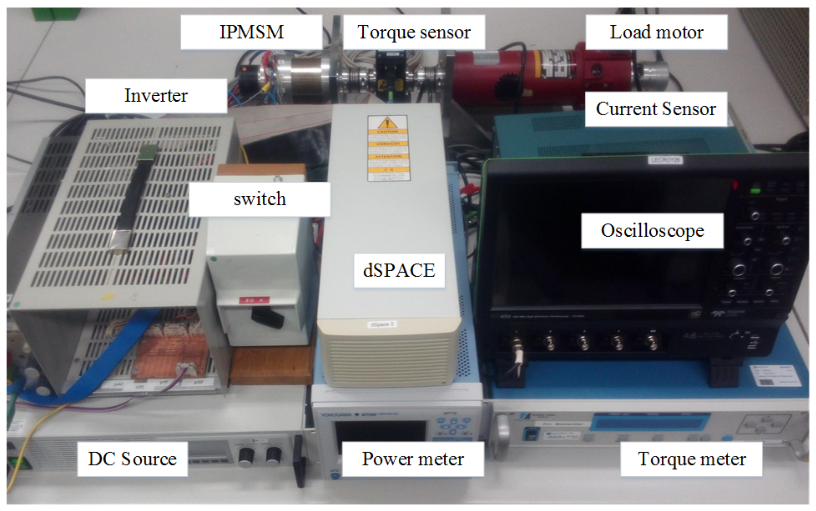
The test bench is shown as Figure 5. The inverter is a specially designed two-level three phase voltage source inverter, the type of the MOSFETS (IXFR180N10, IXYS corporation, Leiden, Netherlands) is IXFR180N10, and the current sensor is T60404-N4646-X100. The parameters of the salient-pole PMSM are shown in Table 1. The ratio between amplitude of back EEMF and speed is very low, which is a severe condition for back EEMF based position sensorless control methods when working in low speed range.
A DC motor is mechanically coupled with the salient-pole PMSM to produce the load torque, an adjustable resistor that connected to the terminal of the DC motor is used to change the load torque. An absolute encoder is used to measure the actual position used for comparison. Both the switching frequency and sampling frequency are 10 kHz.
In the figures shown in the Experimental Results, “Red” represents the reference signals, “Black” means measured signals, “Green” represents the signals that are achieved by using convention method and “Blue” denotes the signals that are obtained by using the proposed method.
4.1. Computation Load Comparison
To evaluate the computational load of the two methods, computation time are compared. In this experiment, the turnaround time is used as a criterion, which can be read directly from the control desk of dSAPCE. The turnaround time includes the communication time, data conversion time, code implementation time and data saving time. Except for code implementation time, the other times of the two methods are the same.
The turnaround time of the two strategies is shown in Table 2. Compared with the conventional method, the time increase of the proposed method is 3.4% of the sampling period.
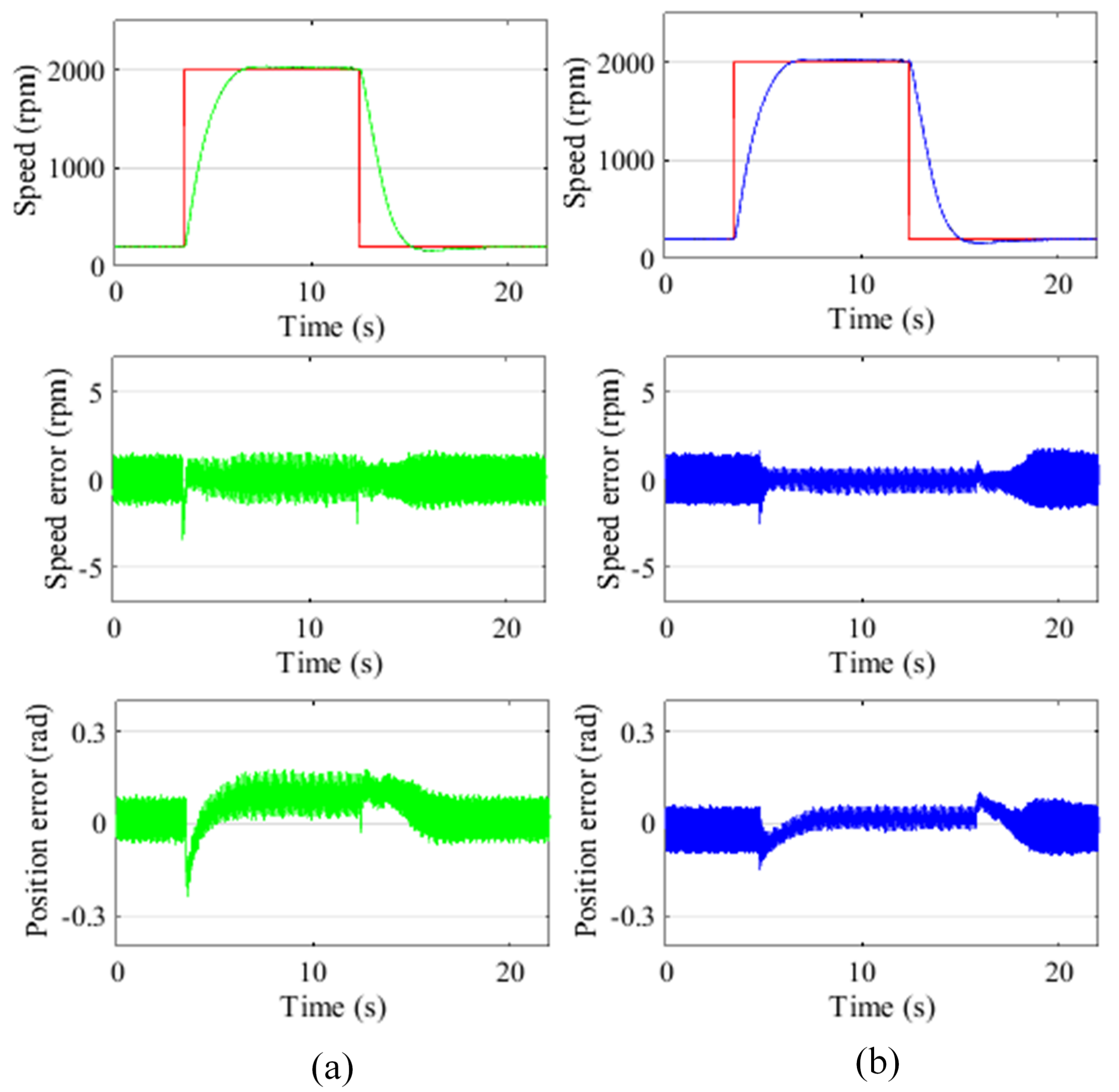
4.2. Speed Variation Comparison
In this experiment, the motor accelerates from 100 rpm to 2000 rpm and then decelerates to 100 rpm without load torque. To make a fair comparison, the switching surface of the proposed method is adjusted to make the estimation error between the proposed method and conventional method is approximately equal at 100 rpm.
During this process, the reference speed, measured speed, estimated speed, speed estimation error and electrical position estimation error are given in Figure 6. The experimental results of the conventional method are shown in Figure 6a, while the experimental results of the proposed method are shown in Figure 6b.
The experimental results show that, at 100 rpm, the speed estimation errors of the two methods are almost the same. With the increase of speed, the speed estimation error of the proposed method is smaller than that of the conventional method. At 2000 rpm, the speed estimation error of the proposed method is about 50% of the conventional method.
At 100 rpm, the electrical rotor position estimation errors of the two methods are similar. During the speed variation process, the maximum electrical rotor position estimation error of the conventional method is −0.2 rad, and the maximum electrical rotor position estimation error of the proposed method is −0.1 rad. At 2000 rpm, the phase lag of the conventional method is 0.1 rad, and the phase lag of the proposed method is zero.
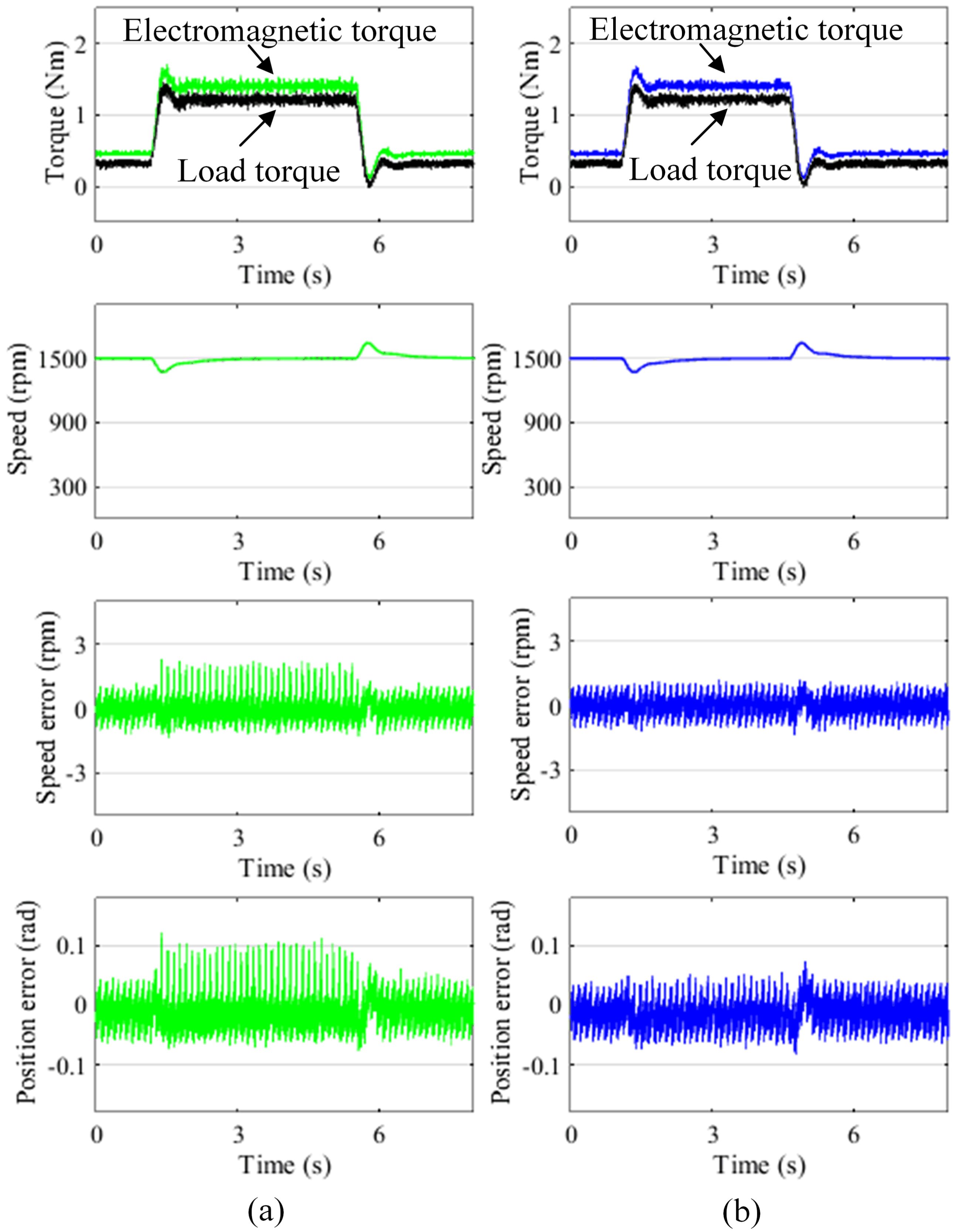
4.3. Torque Variation Comparison
In this experiment, the motor operates under speed control; the speed is 1500 rpm (0.75 p.u.). In the beginning, the load torque is 0.2 Nm (0.1 p.u.), a load torque 1.2 Nm (0.6 p.u.) is provided to the motor as a disturbance, and then the load torque is reduced to 0.2 Nm (0.1 p.u.). During the torque variation process, the electromagnetic torque, load torque, measured speed, estimated speed, electrical position estimation error and speed estimation error are shown as Figure 7.
The experimental results show that, during the torque disturbance process, both the electrical rotor position and speed estimation errors of the proposed method are significantly lower than those of the conventional method.
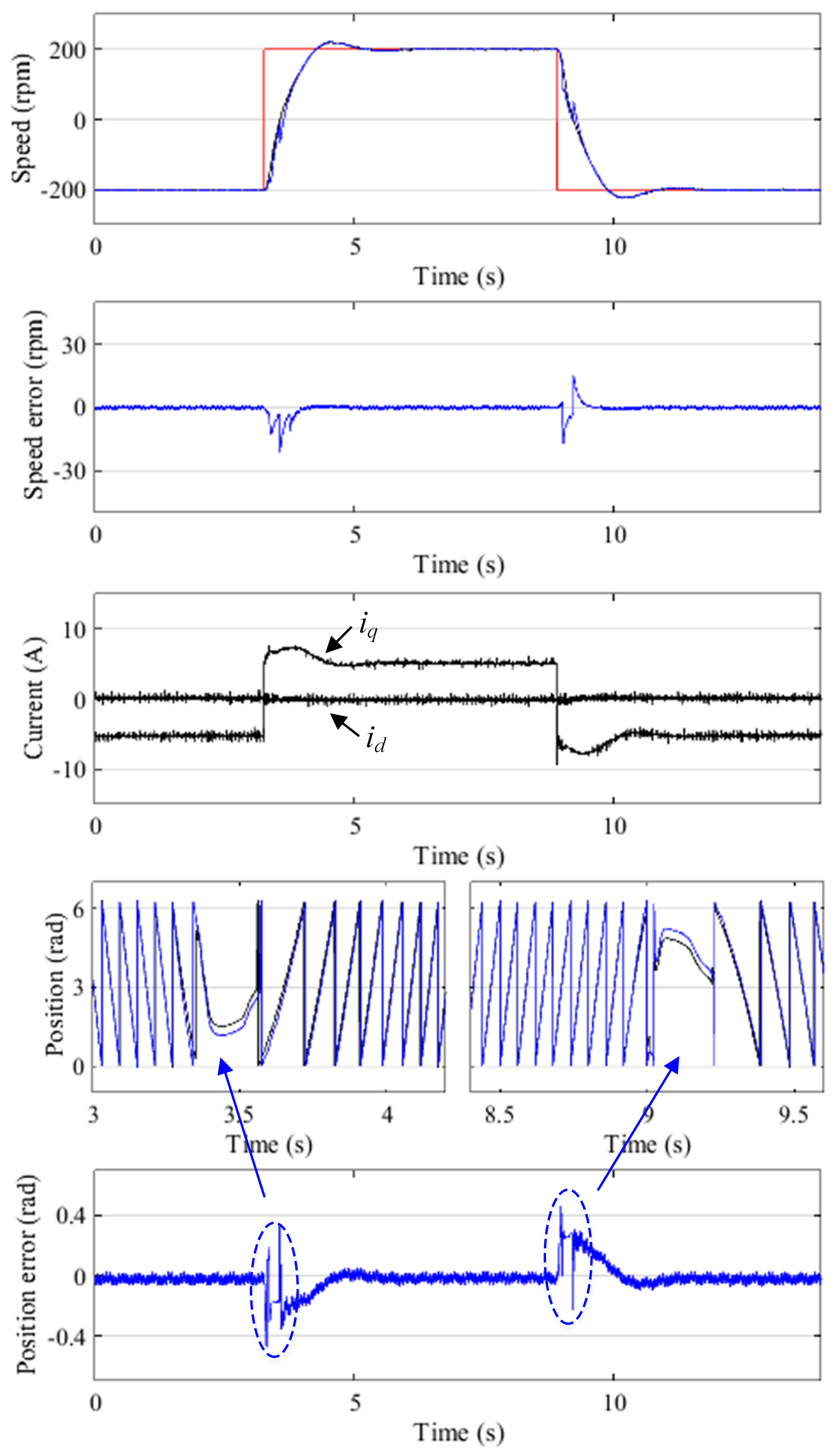
4.4. Speed Reversal
With the conventional full-order discrete-time SMO, the motor can not reverse from one direction to the other without position sensor in this experiment. Therefore, in this section, only the experimental results of the proposed method are shown.
The motor reverses between 200 rpm (0.1 p.u.) and −200 rpm (−0.1 p.u.). The reference speed, measured speed, estimated speed, measured rotor position, estimated rotor position, currents in d-axis and q-axis, speed estimation error and electrical position estimation error are shown in Figure 8.
The experimental results show that the motor can reverse successfully from one direction to the other. During the reversal process, the maximum electrical rotor position and speed estimation errors occur around zero speed. The maximum electrical rotor position estimation error is 0.4 rad, and the maximum rotor speed estimation error is 15 rpm.
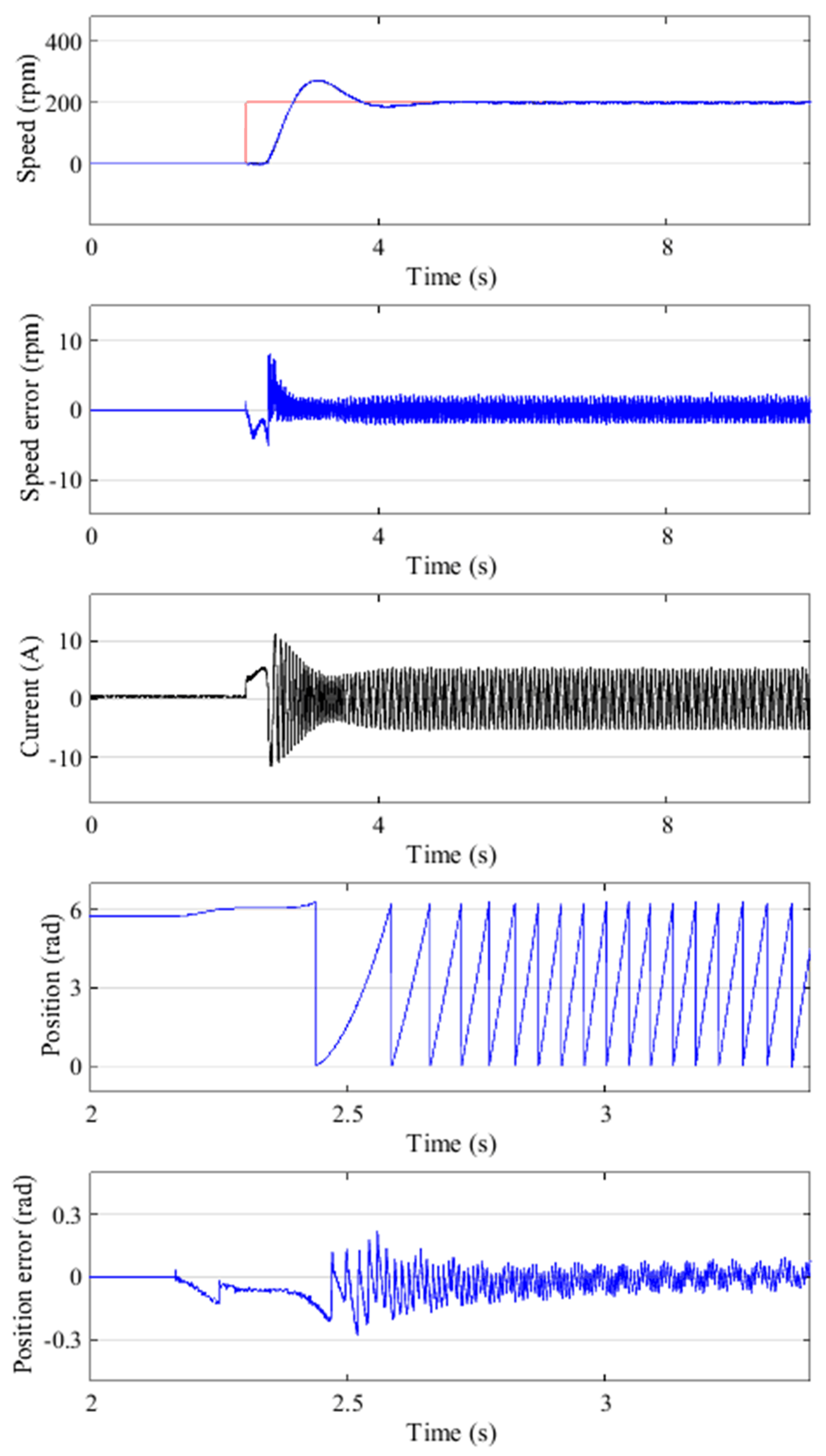
4.5. Start up from Standstill
With the conventional full-order discrete-time SMO, the motor cannot start up from standstill in this experiment. Therefore, in this section, only the experimental results of the proposed method are shown.
The initial rotor position is achieved by initial rotor position Estimation [26]. During the startup process, the reference speed, measured speed, estimated speed, measured rotor position, estimated rotor position, phase current, electrical position estimation error and speed estimation error are shown in Figure 9.
The experimental results show that the motor can start up successfully from standstill. During the startup process, the maximum speed estimation error is 8 rpm and the maximum electrical rotor position estimation error is −0.27 rad.
5. Conclusions
This paper proposes a novel position sensorless control strategy for PMSM considering saliency. A novel full-order SMO is built to estimate the rotor position. The effectiveness of the proposed method is validated on a low voltage salient-pole PMSM.
The performance of a conventional full-order SMO-based position sensorless control method and the proposed method are compared under the same condition. The computational burden of the proposed method is higher than that of the conventional method. In the test bench, the computation time increase is 3.4% of the sampling period. With the rapid development of fast microprocessors, the computational time increase can be ignored.
During speed variation and torque variation process, the performance of the proposed method is obviously better than that of the conventional method. The rotor speed estimation error and position estimation error of the proposed method are about 50% of the conventional method. During speed variations, there is no phase lag in the proposed method. Based on the proposed method, the motor can reverse between positive and negative directions and start up from standstill without a position sensor.
The rotor position is estimated based on the the differential of , so the proposed method can be used for salient-pole PMSM with different load at stand still and low speed. However, due to the restriction of the test bench, it is incapable of producing satisfied load torque at low speed. In the next step, a new test bench will be built to repeat the experiments under heavy mechanical load at zero speed and low speed.
The proposed position sensorless control method can be used for salient-pole PMSMs in electrical car, robot joints, etc., where startup and low speed operation of PMSM are required.
Author Contributions
Y.W. and M.D. designed the position sensorless control method for PMSM. X.W. and W.X. performed the experiments and analyzed the data.
Funding
This research was funded by “the Fundamental Research Funds for the Central Universities”.
Conflicts of Interest
The authors declare no conflict of interest.
References
- Fortino, M.; Víctor, M.; Juvenal, R. Robust speed control of permanent magnet synchronous motors using two-degrees-of-freedom control. IEEE Trans. Ind. Electron. 2018, 65, 6099–6108. [Google Scholar] [CrossRef]
- Zhang, Y.; Xu, D.; Huang, L. Generalized multiple-vector-based model predictive control for PMSM drives. IEEE Trans. Ind. Electron. 2018, 65, 9356–9366. [Google Scholar] [CrossRef]
- Wei, Q.; Xi, Z.; Jin, F.; Hua, B.; Lu, D.; Cheng, B. Using high-control-bandwidth fpga and sic inverters to enhance high-frequency injection sensorless control in interior permanent magnet synchronous machine. IEEE Access 2018, 58, 2169–3536. [Google Scholar] [CrossRef]
- Xu, P.L.; Zhu, Z.Q. Novel square-wave signal injection method using zero-sequence voltage for sensorless control of pmsm drives. IEEE Trans. Ind. Electron. 2016, 63, 7444–7454. [Google Scholar] [CrossRef]
- Ichikawa, S.; Tomita, M.; Doki, S.; Okuma, S. Sensorless control of permanent-magnet synchronous motors using online parameter identification based on system identification theory. IEEE Trans. Ind. Electron. 2016, 53, 363–372. [Google Scholar] [CrossRef]
- Genduso, F.; Miceli, R.; Rando, C.; Galluzzo, G.R. Back EMF sensorless-control algorithm for high-dynamic performance PMSM. IEEE Trans. Ind. Electron. 2010, 57, 2092–2100. [Google Scholar] [CrossRef]
- Bolognani, S.; Tubiana, L.; Zigliotto, M. Extended kalman filter tuning in sensorless pmsm drives. IEEE Trans. Ind. Appl. 2013, 39, 1741–1747. [Google Scholar] [CrossRef]
- Fuentes, E.; Kennel, R. Sensorless-predictive torque control of the pmsm using a reduced order extended kalman filter. Symp. Sensorless Control Electron. Drives (SLED) 2011, 39, 123–128. [Google Scholar] [CrossRef]
- Junggi, L.; Jinseok, H.; Kwanghee, N.; Ortega, R.; Praly, L.; Astolfi, A. Sensorless control of surface-mount permanent-magnet synchronous motors based on a nonlinear observer. IEEE Trans. Power Electron. 2010, 25, 290–297. [Google Scholar] [CrossRef] [Green Version]
- Foo, G.H.B.; Rahman, M.F. Direct torque control of an ipmsynchronous motor drive at very low speed using a sliding-mode stator flux observer. IEEE Trans. Power Electron. 2010, 25, 933–942. [Google Scholar] [CrossRef]
- Zhao, Y.; Qiao, W.; Wu, L. Position extraction from a discrete sliding-mode observer for sensorless control of ipmsms. IEEE Int. Symp. Ind. Electron. 2012, 25, 725–730. [Google Scholar] [CrossRef]
- Foo, G.; Rahman, M.F. Sensorless sliding-mode mtpa control of an ipm synchronous motor drive using a sliding-mode observer and hf signal injection. IEEE Trans. Ind. Electron. 2010, 57, 1270–1278. [Google Scholar] [CrossRef]
- Zhao, Y.; Qiao, W.; Wu, L. An adaptive quasi-sliding-mode rotor position observer-based sensorless control for interior permanent magnet synchronous machines. IEEE Trans. Power Electron. 2013, 28, 5618–5629. [Google Scholar] [CrossRef]
- Yue, Z.; Zhe, Z.; Wei, Q.; Long, W. An extended flux model-based rotor position estimator for sensorless control of salient-pole permanentmagnet synchronous machines. IEEE Trans. Power Electron. 2015, 30, 4412–4422. [Google Scholar] [CrossRef]
- Guoqiang, Z.; Gaolin, W.; Ronggang, N.; Dianguo, X. Active flux based full-order discrete-time sliding mode observer for position sensorless ipmsm drives. In Proceedings of the 2014 17th International Conference on Electrical Machines and Systems (ICEMS), Hangzhou, China, 22–25 October 2014. [Google Scholar] [CrossRef]
- Feng, Y.; Zheng, J.; Yu, X.; Truong, N.V. Hybrid terminal slidingmode observer design method for a permanent-magnet synchronous motor control system. IEEE Trans. Ind. Appl. 2009, 56, 3424–3431. [Google Scholar] [CrossRef]
- Kim, M.; Sul, S.K. An enhanced sensorless control method for pmsm in rapid accelerating operation. In Proceedings of the 2010 International Power Electronics Conference-ECCE ASIA, Sapporo, Japan, 21–24 June 2010. [Google Scholar] [CrossRef]
- Ackermann, J.; Utkin, V. Sliding mode control design based on ackermann’s formula. IEEE Trans. Autom. Control 2009, 43, 234–237. [Google Scholar] [CrossRef]
- Ramon, G.; Luis, G.; Miguel, C.; Jaume, M.; Helena, M. Variable structure control in natural frame for three-phase grid-connected inverters with LCL filter. IEEE Trans. Power Electron. 2018, 33, 4512–4522. [Google Scholar] [CrossRef]
- Zhu, Q.; Wang, T.; Jiang, M.; Wang, Y. A new design scheme for discrete-time variable structure control systems. In Proceedings of the 2009 International Conference on Mechatronics and Automation, Changchun, China, 9–12 August 2009. [Google Scholar] [CrossRef]
- Ma, H.; Wu, J.; Xiong, Z. A novel exponential reaching law of discrete-time sliding-mode control. IEEE Trans. Ind. Electron. 2017, 64, 3840–3850. [Google Scholar] [CrossRef]
- Wang, G.; Li, Z.; Zhang, G.; Yu, Y.; Xu, D. Quadrature PLL-based high-order sliding-mode observer for IPMSM sensorless control with online MTPA control strategy. IEEE Trans. Ind. Electron. 2013, 28, 214–224. [Google Scholar] [CrossRef]
- Comanescu, M. Cascaded EMF and speed sliding mode observer for the nonsalient PMSM. In Proceedings of the IECON 2010-36th Annual Conference on IEEE Industrial Electronics Society, Glendale, AZ, USA, 7–10 November 2010. [Google Scholar] [CrossRef]
- DeCarlo, R.A.; Zak, S.H.; Matthews, G.P. Variable structure control of nonlinear multivariable systems: A tutorial. Proc. IEEE 2013, 76, 212–232. [Google Scholar] [CrossRef]
- Hoseinnezhad, R.; Harding, P. A novel hybrid angle tracking observer for resolver to digital conversion. In Proceedings of the 44th IEEE Conference on Decision and Control, Seville, Spain, 15 December 2005. [Google Scholar] [CrossRef]
- Wu, X.; Feng, Y.; Liu, X.; Huang, S.; Yuan, X.; Gao, J.; Zheng, J. Initial rotor position detection for sensorless interior pmsm with square-wave voltage injection. IEEE Trans. Magn. 2017, 53, 1–4. [Google Scholar] [CrossRef]
Figure 1.
Illustration of the salient-pole permanent magnet synchronous motor (PMSM) model.

Figure 2.
Sliding mode observer diagram.

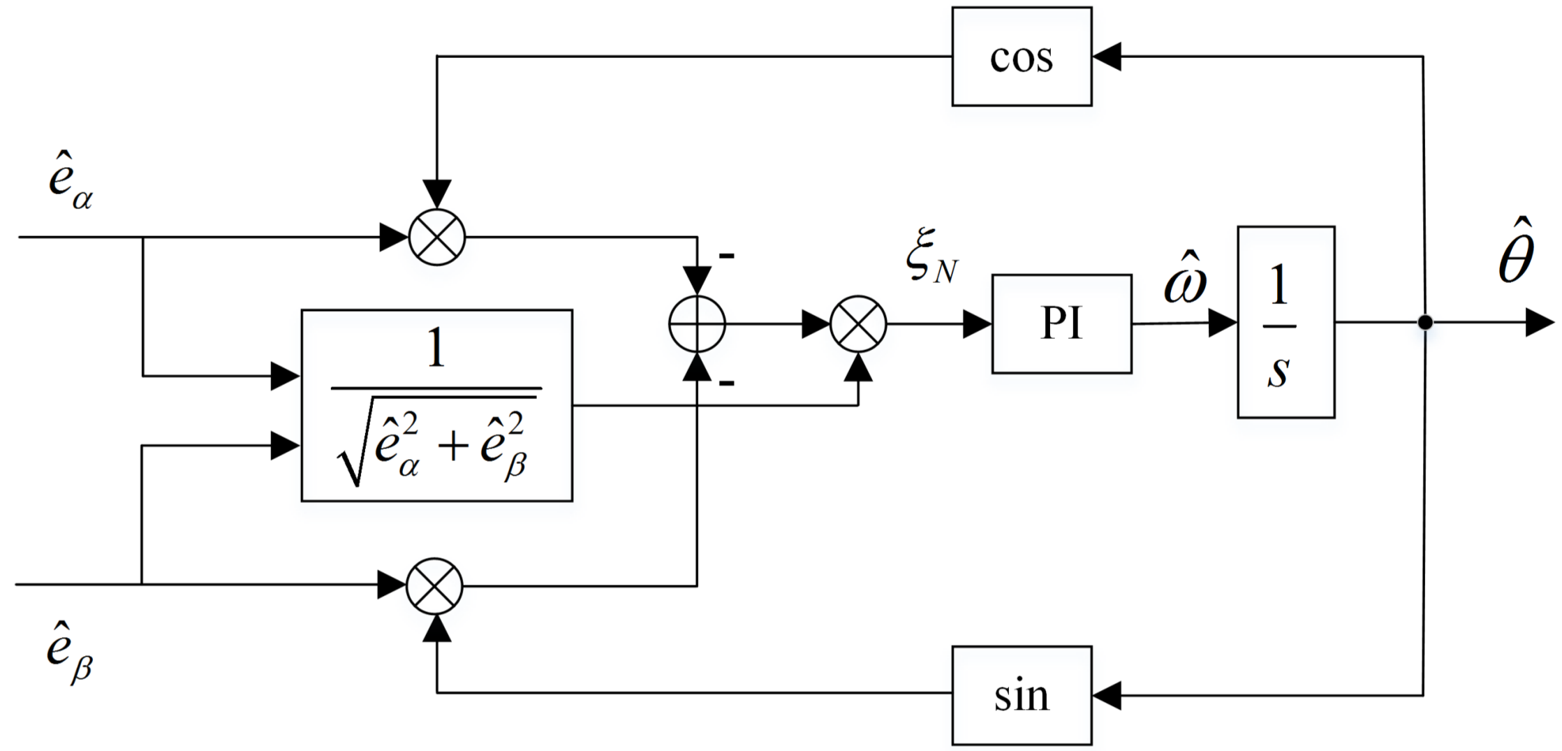
Figure 3.
Angle-tracking observer.

Figure 4.
Rotor position and speed estimation diagram.

Figure 5.
The test bench.

Figure 6.
The speed changes from 100 rpm (0.05 p.u.) to 2000 rpm (1 p.u.): (a) conventional method; and (b) proposed method. “Red Line” represents the reference signals, “Green Line” represents the signals that are achieved by using convention method and “Blue Line” denotes the signals that are obtained by using the proposed method.

Figure 7.
The load torque changes from 0.2 Nm (0.1 p.u.) to 1.2 Nm (0.6 p.u.): (a) conventional method; and (b) proposed method. “Black Line” means measured signals, “Green Line” represents the signals that are achieved by using convention method and “Blue Line” denotes the signals that are obtained by using the proposed method.

Figure 8.
The speed changes between 200 rpm (0.1 p.u.) and −200 rpm (−0.1 p.u.). “Red Line” represents the reference signals, “Black” means measured signals and “Blue Line” denotes the signals that are obtained by using the proposed method.
Figure 8.
The speed changes between 200 rpm (0.1 p.u.) and −200 rpm (−0.1 p.u.). “Red Line” represents the reference signals, “Black” means measured signals and “Blue Line” denotes the signals that are obtained by using the proposed method.

Figure 9.
The motor starts up from zero speed to 200 rpm (0.1 p.u.).


Table 1.
Parameters of the tested IPMSM.
| Parameter | Value |
|---|---|
| Rated torque | 2 Nm |
| Rated current/voltage (rms) | 50 A/13 V |
| Number of pole pairs | 5 |
| -axis inductance | 0.05/0.095 mH |
| Resistance | 18 mΩ |
| Rated speed | 2000 rpm |
| The moment of inertia | 0.00187 kg·m2 |
| PM flux linkage | 0.00707 Vs |
Table 2.
Turnaround time comparison of the conventional method and the proposed method.
| Time | Value |
|---|---|
| Conventional method (μs) | 8.9 |
| Proposed method (μs) | 12.3 |
| Increased time (μs) | 3.4 |
| Sampling period (μs) | 100 |
| Increased time percentage | 3.4% |
© 2018 by the authors. Licensee MDPI, Basel, Switzerland. This article is an open access article distributed under the terms and conditions of the Creative Commons Attribution (CC BY) license (http://creativecommons.org/licenses/by/4.0/).
Share and Cite
MDPI and ACS Style
Wang, Y.; Wang, X.; Xie, W.; Dou, M. Full-Speed Range Encoderless Control for Salient-Pole PMSM with a Novel Full-Order SMO. Energies 2018, 11, 2423. https://doi.org/10.3390/en11092423
AMA Style
Wang Y, Wang X, Xie W, Dou M. Full-Speed Range Encoderless Control for Salient-Pole PMSM with a Novel Full-Order SMO. Energies. 2018; 11(9):2423. https://doi.org/10.3390/en11092423
Chicago/Turabian StyleWang, Yuanlin, Xiaocan Wang, Wei Xie, and Manfeng Dou. 2018. "Full-Speed Range Encoderless Control for Salient-Pole PMSM with a Novel Full-Order SMO" Energies 11, no. 9: 2423. https://doi.org/10.3390/en11092423
Note that from the first issue of 2016, this journal uses article numbers instead of page numbers. See further details here.