A Novel Adaptive Neuro-Control Approach for Permanent Magnet Synchronous Motor Speed Control

Abstract

A speed controller for permanent magnet synchronous motors (PMSMs) under the field oriented control (FOC) method is discussed in this paper. First, a novel adaptive neuro-control approach, single artificial neuron goal representation heuristic dynamic programming (SAN-GrHDP) for speed regulation of PMSMs, is presented. For both current loops, PI controllers are adopted, respectively. Compared with the conventional single artificial neuron (SAN) control strategy, the proposed approach assumes an unknown mathematic model of the PMSM and guides the selection value of parameter K online. Besides, the proposed design can develop an internal reinforcement learning signal to guide the dynamic optimal control of the PMSM in the process. Finally, nonlinear optimal control simulations and experiments on the speed regulation of a PMSM are implemented in Matlab2016a and TMS320F28335, a 32-bit floating-point digital signal processor (DSP), respectively. To achieve a comparative study, the conventional SAN and SAN-GrHDP approaches are set up under identical conditions and parameters. Simulation and experiment results verify that the proposed controller can improve the speed control performance of PMSMs.

1. Introduction

Permanent magnet synchronous motors (PMSMs) have many advantages, such as high power density, simple structure, small volume, high efficiency and reliability. PMSMs are widely used in numerical control machine tools, aerospace and industrial robotic manipulators [1]. A PMSM is a typical nonlinear and strongly coupled system, with unpredictable external disturbances, as well as internal parameter variations [2]. In recent years, various nonlinear control methods [3,4,5,6,7,8,9,10,11], such as fuzzy logic control, sliding mode control, neural network control, nonlinear optimal control, internal model control, adaptive control, have been used to meet the requirements of high reliability and performance in PMSM control [7,8,9,10]. The fuzzy logic control is successfully applied in the speed control of PMSMs [12,13]. However, the fuzzy control membership function is mainly based on expert experience, which is difficult to obtain. Sliding mode control is a preferred research topic, due to its insensitivity to variation of control object parameters and load disturbances [14,15]. Nevertheless, chattering phenomena exist in this control method. Meanwhile, nonlinear optimal control has been put forward as a new PMSM control method [16]. However, the parameters of the PMSM must be sufficiently accurate, and control results cannot adapt in time when the mechanical parameters of PMSM change. In [17], a novel control scheme combining the inverse system method and the internal model control for a bearingless permanent magnet synchronous motor (BPMSM) was proposed by Sun et al., although in order to regulate the tracking and disturbance rejection properties, the values of control parameter sets need to be adjusted separately [18].

Recently, adaptive dynamic programming (ADP) has attracted significantly increasing attention as a novel level reinforcement learning approach. It can solve the “curse of dimensionality” of conventional dynamic programming by approximately computing cost function [19]. ADP can be categorized into three classical structures [20]: the first is heuristic dynamic programming (HDP), the second is dual heuristic dynamic programming (DHP), and the last is globalized dual heuristic dynamic programming (GDHP). The main difference is that the critic network is used to approximate the value function J in HDP, while it is used to approximate the derivatives of value function J in DHP. GDHP incorporates the benefits of HDP and DHP, by approximating both value function J and its derivatives, respectively.

In paper [21], a novel hierarchical structure of ADP approach named goal representation heuristic dynamic programming (GrHDP) is proposed. Compared with the conventional ADP approach, the proposed approach has an additional reference network which can automatically build an internal reinforcement signal to facilitate the optimal learning, control effectively and efficiency [22]. This novel hierarchical ADP approach is of a superior learning performance over the traditional ones. The GrHDP approach is used in various fields of electrical engineering, such as power system stability control for a wind farm [23], power oscillation damping control for superconducting magnetic energy storage [24], and load frequency control for an islanded smart grid [25].

Meanwhile, the single artificial neuron (SAN) control approach has been used in many applications for its robust control in the presence of noise and uncertainties [26]. Generally speaking, traditional SAN control has been applied to engineering practices for a long time due to its good performance and easy implementation [27,28,29].

It has been pointed out that although the conventional SAN control approach can provide an online learning ability for the PMSM parameter variation, it may not provide a satisfactory property of load disturbance rejection. The reason is that the control effect of SAN mainly depends on the parameter K (neuron scale-up factor). The parameter K is very important to the control response performance. The selection of K is very difficult in traditional SAN control approaches. The control system will respond faster if the K value increases. However, the K value will lead to the instability of the system, if it is out of a certain range. Moreover, there is no profound theoretical background, which can be used to tune the parameter K for complicated systems with uncertainties and disturbance. It is a new idea to use machine learning to adjust the K value of SAN and make it applicable to PMSM control. At the same time, for the ultimate convergence, the action network weights of GrHDP approach usually need repeating online learning to achieve optimization solutions to the Bellman equation. So far, articles about ADP approaches mostly focus on the simulation stage [23,24,30,31,32,33,34,35,36].

To solve the above problems, in this paper, a novel neuro-control framework using GrHDP and SAN is proposed. Moreover, an application study on PMSM vector control system is also presented in this research. The main contributions of this paper are summarized as follows:

(1)

A novel adaptive neuro-control controller, called single artificial neuron goal representation heuristic dynamic programming (SAN-GrHDP), based on SAN and GrHDP has been proposed in this paper. This framework, under which the parameter K in the SAN has been updated through a reference learning mechanism, can provide a sequential online control policy.

(2)

The formula of SAN-GrHDP approach is derived, and the reinforcement signal and learning process are designed for the vector control of PMSM. Simulation studies have been carried out for the proposed approach. Simulation results demonstrate that the proposed controller has a higher potential of disturbance rejection, with much less speed fluctuation and shorter recovering time towards load disturbance.

(3)

Moreover, comparative experiments of original SAN and SAN-GrHDP approaches are performed on the speed control of PMSM under the same conditions and parameters. The results of the experiments verify that SAN-GrHDP can better improve the control effect by interacting with the control object, and has much better robustness than SAN with load mutation and load disturbance.

The remainder of the paper is organized as follows. Section 2 describes the servo control system of a PMSM as well as the certain modeling of the speed controller used in this paper. Section 3 illustrates the details of the SAN-GrHDP controller, and the learning algorithm associated. In Section 4, the simulation of the speed control of the PMSM and the experimental setup based on SAN-GrHDP are presented. The results prove the effectiveness of the proposed SAN-GrHDP by comparing with the conventional SAN control approach. Finally, Section 5 presents our conclusions and a few future study directions.

2. Model of Permanent Magnet Synchronous Motor Control System

Assuming that magnetic circuit saturation, hysteresis eddy current losses are disregarded and the sinusoidal magnetic field is distributed in space, a surface-mounted PMSM is considered as the controlled object. In d-q coordinates, the model of a surface mounted PMSM can be expressed as follows [37,38]:

$$\left(\begin{array}{l}{i}_d{}^{\prime }\\ i_q{}^{\prime }\\ {\omega }^{\prime }\end{array}\right)=\left(\begin{array}{ccc}-\frac{R_s}{L_d}& n_p\omega & 0\\ -n_p\omega & -\frac{R_s}{L_d}& -\frac{n_p{\psi }_f}{L_q}\\ 0& -\frac{1.5n_p{\psi }_f}{J}& -\frac{B}{J}\end{array}\right)\left(\begin{array}{l}{i}_d\\ i_q\\ \omega \end{array}\right)+\left(\begin{array}{l}\frac{u_d}{L_d}\\ \frac{u_q}{L_q}\\ -\frac{T_L}{J}\end{array}\right)$$

(1)

where $u_d$ and $u_q$ are the stator d- and q-axes voltages, $i_d$ and $i_q$ are the stator d- and q-axes currents, $L_d$ and $L_q$ are the stator d- and q-axes inductances, $n_p$ is the number of pole pairs, $R_s$ is the stator resistance, $\omega$ is the rotor angular velocity, ${\psi }_f$ is the flux linkage, $T_L$ is the load torque, and B is the viscous friction coefficient.

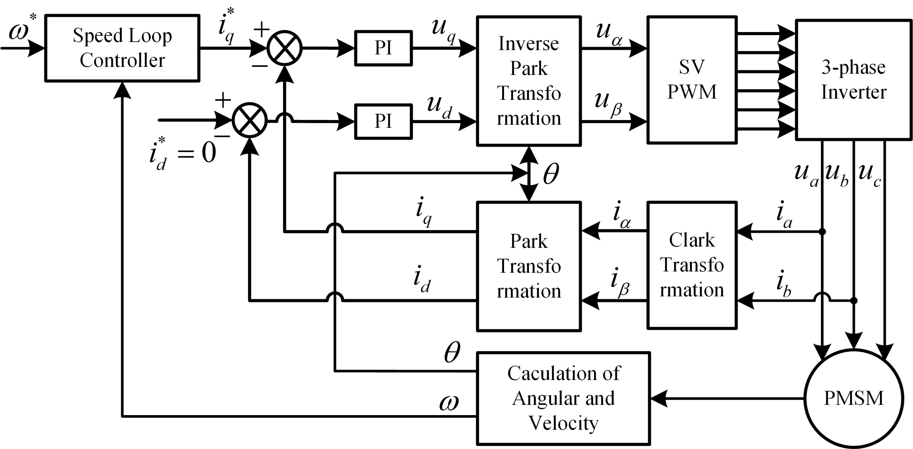
The strategies of the vector control of PMSM have $i_d=0$ control, power factor $\cos \varphi =1$ control, the maximum torque control, maximum output power control, flux weakening control and so on. The approach of $i_d=0$ control which has many advantages such as small torque ripple and wide speed range, is the most simple strategy of vector control and used in this article. The field oriented control (FOC) diagram of PMSM system by $i_d=0$ control approach is shown in Figure 1. There are three controllers in the diagram: one speed tracking loop controller and two current tracking loop controllers. The d- and q-axes currents $i_d$, $i_q$ can be calculated from the two-phase static coordinate currents $i_{\alpha }$, $i_{\beta }$ of PMSM by the PARK transform. Similarly, the $i_{\alpha }$, $i_{\beta }$ currents can be obtained from the actual phase currents of PMSM through the CLARK transform. The rotor angular velocity $\omega$ and rotor position $\theta$ can be calculated from encoder. Usually, the reference current value $i_q^{*}$ is determined by the speed loop controller output, and $i_d^{*}$ is set to zero. Due to saturation phenomena of PMSMs, some values can depend on the operating point of the machine, such as rotor inductance and rotor resistance. This can affect the performance and the accuracy of the conventional controller. The SAN-GrHDP approach is a kind of machine learning algorithm (ADP approach). When motor parameters change, the controller can learn from a complex, uncertain environment (controlled plant) according to the optimal cost function, which is also the essence of ADP method [19]. Compared with the traditional control approach, the SAN-GrHDP can realize self-regulation by critic network and provide an online sequential control policy, not subject to the external load disturbances and parameter variations. This article mainly discusses the external load disturbances rejection capacity of proposed control strategy. The current-loop sampling period is 200 $\mathsf{\mu }\mathrm{s}$, and the speed-loop sampling time is ten times that of the current-loop. The current-loop controllers require faster response. Therefore, the inner current-loop controllers adopt the traditional PI controllers. Here, the task is to design a speed controller based on SAN-GrHDP approach.

3. Single Artificial Neuron Goal Representation Heuristic Dynamic Programming Controller

Like the conventional GrHDP approach [21,39,40], the proposed SAN-GrHDP controller also includes three approximate networks: an action network, a critic network, and a reference network. The critic network is set to approximate the cost-to-go function in Bellman equation by online learning. The reference network provides an adaptive internal reinforcement signal to facilitate the critic network to better approximate the value function. Compared with the classic ADP structure, GrHDP approach has an additional reference network to generate an internal goal-representation signal to facilitate learning and optimization. It provides an effective method for the intelligent system to achieve the goals by adaptive and automatic construction of internal goal representations [21]. This structure, due to the addition of reference network, also has some disadvantages, such as complex structure and high computation burden.

However, the action network of conventional GrHDP approach must be trained many times to ensure the convergence of weights. Because the action network is BP network, and it is difficult to use the conventional GrHDP approach for real-time control, especially in the field of PMSM speed control. In this article, the traditional GrHDP approach is improved and the action network is replaced by SAN control approach. Different from that of the conventional SAN control approach, the parameter K of the action network (SAN) is not fixed, and can be updated through interaction with controlled object in real time.

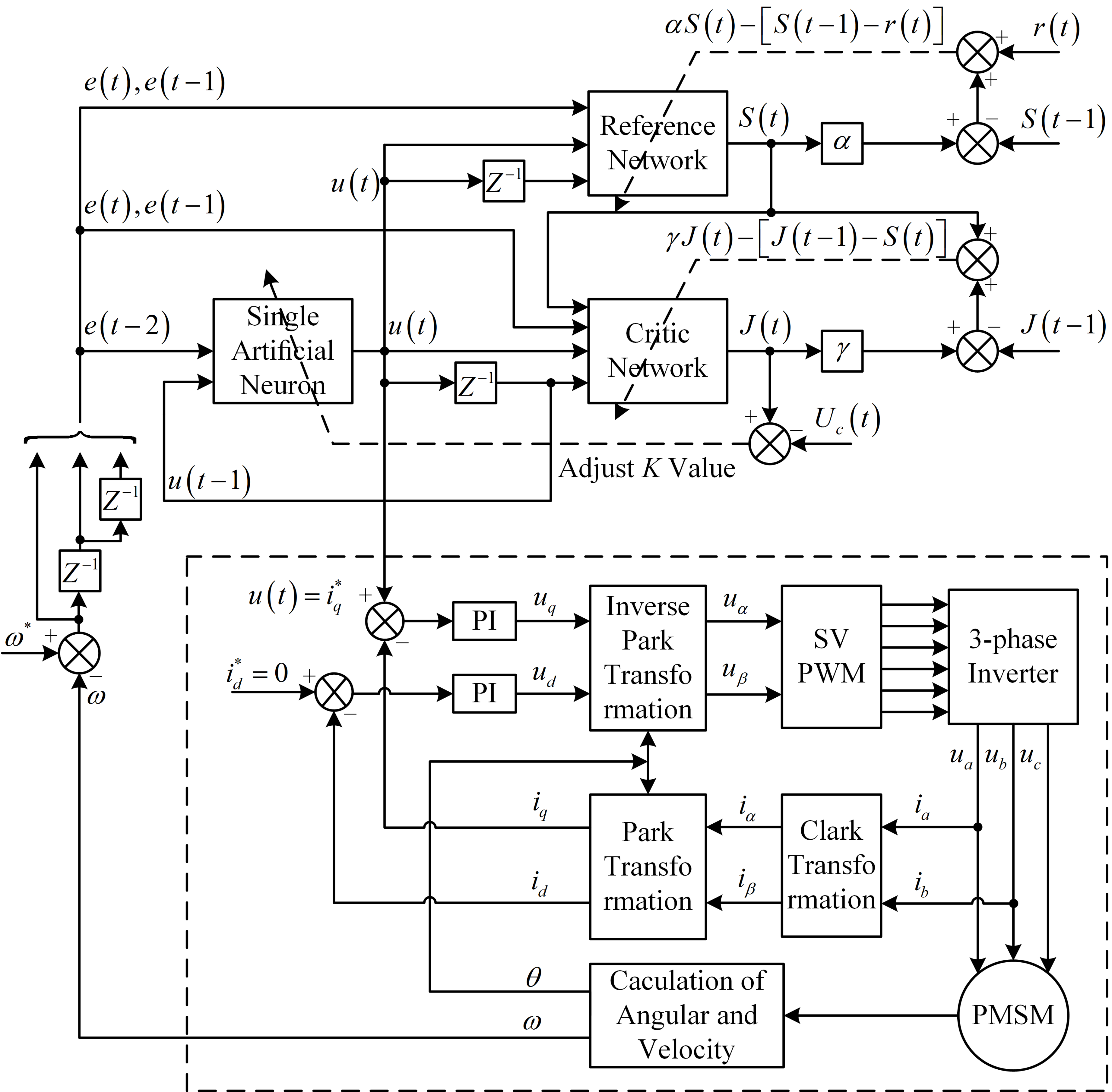
The schematic diagram of FOC by proposed SAN-GrHDP is shown in Figure 2. The ultimate objective for the SAN-GrHDP controller is still to solve the Bellman’s optimal equation [20,22] as:

$$J^{*}\left(x,u\right)=\underset{u}{\min }\left(r\left(x,u\right)+\alpha J^{*}\left(x^{\prime },u^{\prime }\right)\right)$$

(2)

so that the optimal control strategy can be achieved. Here the $J^{*}\left(x,u\right)$ is the immediate cost incurred by u at current time, the $J^{*}\left(x^{\prime },u^{\prime }\right)$ is refer to the one-step future cost, the $\alpha$ is a discounted factor (0 < $\alpha$ < 1), and the $r\left(x,u\right)$ is the external reinforcement signal.

Compared with conventional SAN control approach, the SAN-GrHDP approach has two additional networks (i.e., the reference network and the critic network). The reference network is related to the primary reinforcement signal $r\left(t\right)$, and generates the internal reinforcement signal $S\left(t\right)$ to facilitate the critic network to better approximate the value function. The critic network generates the cost function $J\left(t\right)$, according to $S\left(t\right)$.

3.1. Learning and Adaptation of Reference Network

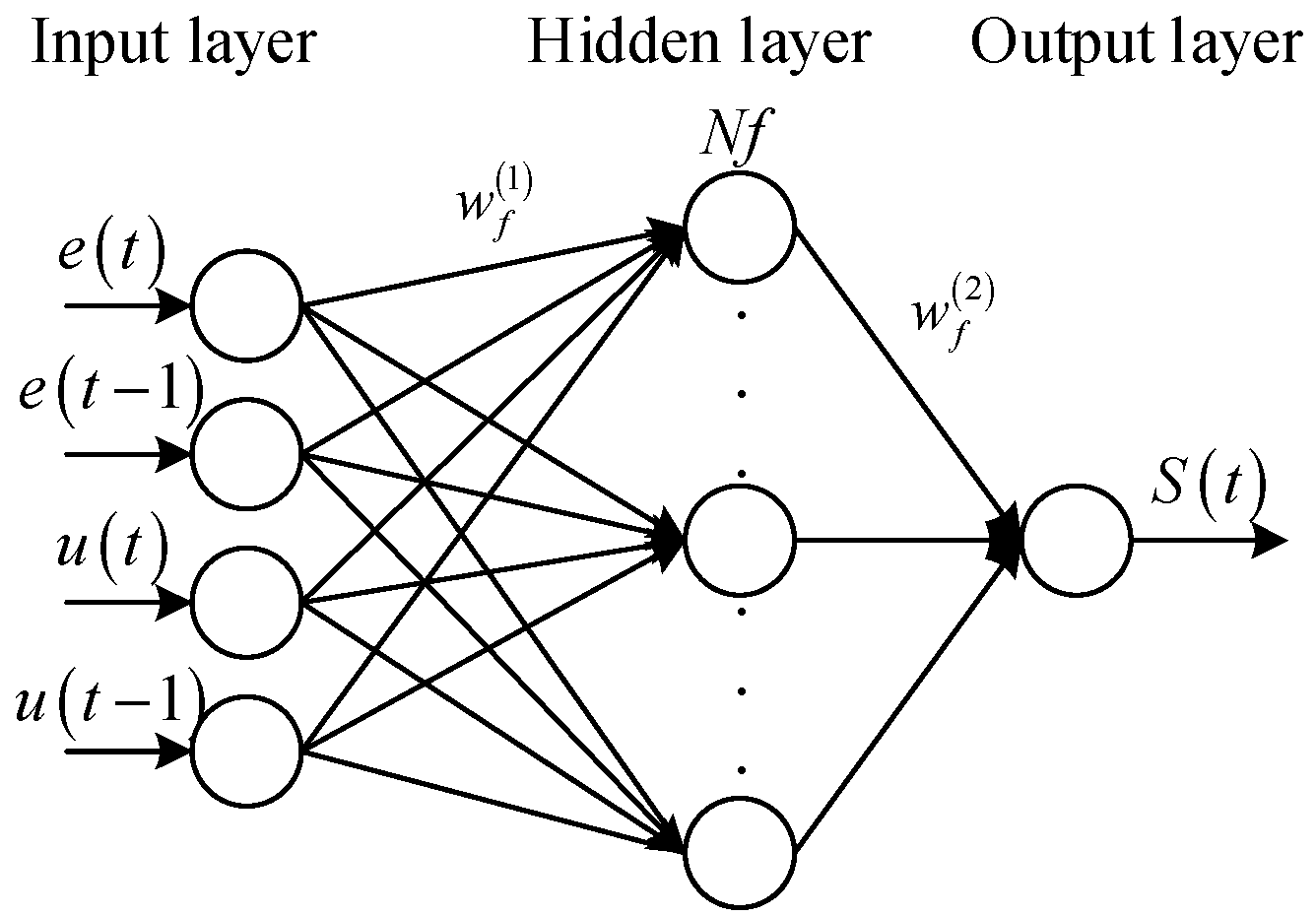
The structure of the reference network is shown in Figure 3. It can be seen that the reference network is designed with three-layer nonlinear architecture (including one hidden layer).

The feed-forward propagation formulas of the reference network are as follows:

$$S\left(t\right)={\displaystyle \sum _{i=1}^{Nf}{w}_{f_i}^{\left(2\right)}\left(t\right)p_i\left(t\right)}i=1,\dots ,Nf$$

(3)

$$p_i\left(t\right)=\frac{1-{\exp }^{-q_i\left(t\right)}}{1+{\exp }^{-q_i\left(t\right)}}i=1,\dots ,Nf$$

(4)

$$q_i\left(t\right)={\displaystyle \sum _{j=1}^4{w}_{f_{i,j}}^{\left(1\right)}\left(t\right)a_j\left(t\right)}i=1,\dots ,Nf$$

(5)

$$a\left(t\right)={\left[e\left(t\right),e\left(t-1\right),u\left(t\right),u\left(t-1\right)\right]}^{{\rm T}}$$

(6)

where $a\left(t\right)$ is the input vector of the reference network whose number is 4, including error value $e\left(t\right)$ at time t, error value $e\left(t-1\right)$ at time t − 1, action value $u\left(t\right)$ at time t, and action value $u\left(t-1\right)$ at time t − 1. $q_i\left(t\right)$ is the ith hidden node input of the reference network. $p_i\left(t\right)$ is the corresponding output of the hidden node. Nf is the total number of the hidden nodes. $S\left(t\right)$ is the output of the reference network.

We define the error function of the reference network as [25]:

$$e_f\left(t\right)=\alpha S\left(t\right)-\left[S\left(t-1\right)-r\left(t\right)\right]$$

(7)

and the objective function to be minimized as:

$$E_f\left(t\right)=\frac{1}{2}{e}_f^2\left(t\right)$$

(8)

To calculate the back propagation through the chain rule, the weights updating rules can be presented as follows [25]:

$\Delta w_f^{\left(2\right)}\left(t\right)$ (the weights adjustments of reference network for the hidden to the output layer):

$$\Delta w_{f_i}^{\left(2\right)}\left(t\right)=l_f\left(t\right)\left[-\frac{\partial E_f\left(t\right)}{\partial w_{f_i}^{\left(2\right)}\left(t\right)}\right]$$

(9)

$$\frac{\partial E_f\left(t\right)}{\partial w_{f_i}^{\left(2\right)}\left(t\right)}=\frac{\partial E_f\left(t\right)}{\partial e_f\left(t\right)}\frac{\partial e_f\left(t\right)}{\partial S\left(t\right)}\frac{\partial S\left(t\right)}{\partial w_{f_i}^{\left(2\right)}\left(t\right)}=\alpha e_f\left(t\right)p_i\left(t\right)$$

(10)

$\Delta w_f^{\left(1\right)}\left(t\right)$ (the weights adjustments of reference network for the input to the hidden layer):

$$\Delta w_{f_{i,j}}^{\left(1\right)}\left(t\right)=l_f\left(t\right)\left[-\frac{\partial E_f\left(t\right)}{\partial w_{f_{i,j}}^{\left(1\right)}\left(t\right)}\right]$$

(11)

$$\frac{\partial E_f\left(t\right)}{\partial w_{f_{i,j}}^{\left(1\right)}\left(t\right)}=\frac{\partial E_f\left(t\right)}{\partial e_f\left(t\right)}\frac{\partial e_f\left(t\right)}{\partial S\left(t\right)}\frac{\partial S\left(t\right)}{\partial p_i\left(t\right)}\frac{\partial p_i\left(t\right)}{\partial q_i\left(t\right)}\frac{\partial q_i\left(t\right)}{\partial w_{f_{i,j}}^{\left(1\right)}\left(t\right)}=\alpha e_f\left(t\right)w_{f_i}^{\left(2\right)}\left[\frac{1}{2}\left(1-p_i^2\left(t\right)\right)\right]a_j\left(t\right)$$

(12)

3.2. Learning and Adaptation of Critic Network

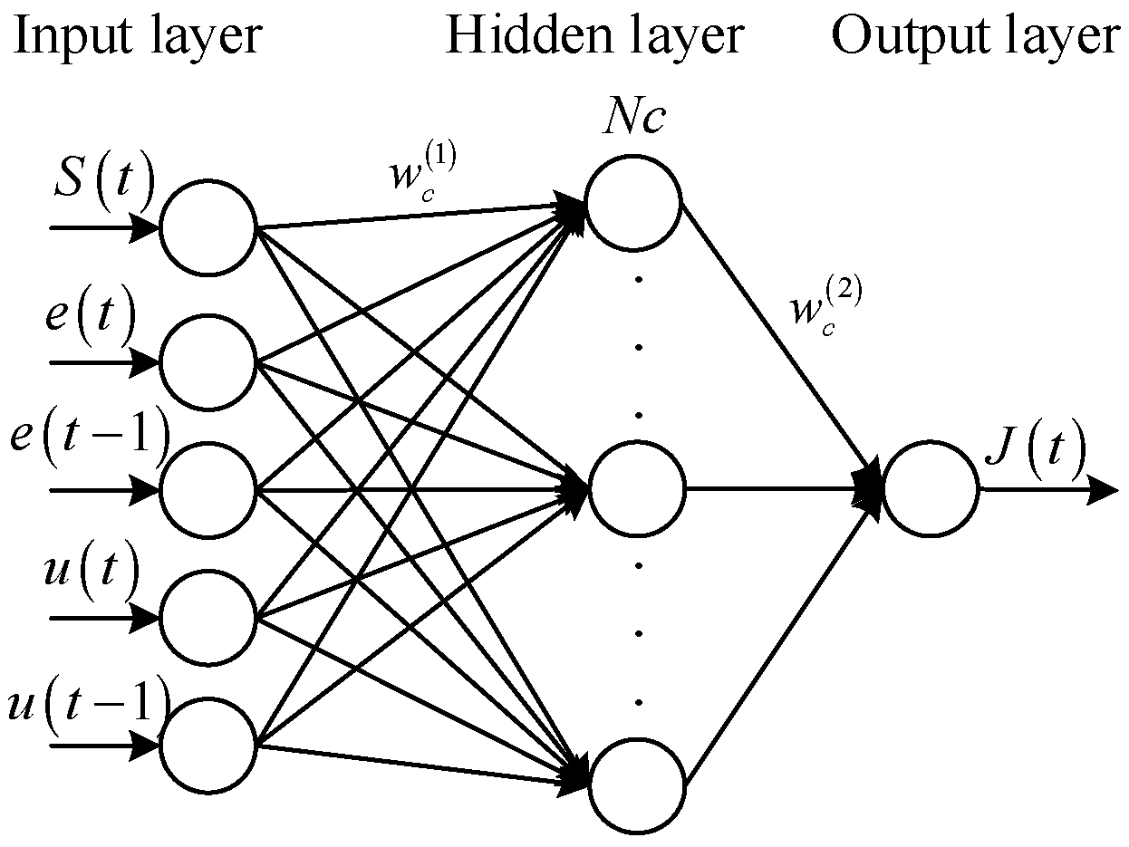
The structure of the critic network is shown in Figure 4. It is designed with a three-layer nonlinear architecture (with one hidden layer).

The feed-forward propagation formulas of the critic network are as follows:

$$J\left(t\right)={\displaystyle \sum _{l=1}^{Nc}{w}_{c_l}^{\left(2\right)}\left(t\right)y_l\left(t\right)}l=1,\dots ,Nc$$

(13)

$$y_l\left(t\right)=\frac{1-{\exp }^{-z_l\left(t\right)}}{1+{\exp }^{-z_l\left(t\right)}}l=1,\dots ,Nc$$

(14)

$$z_l\left(t\right)={\displaystyle \sum _{k=1}^5{w}_{c_{l,k}}^{\left(1\right)}\left(t\right)c_k\left(t\right)}l=1,\dots ,Nc$$

(15)

$$c\left(t\right)={\left[S\left(t\right),e\left(t\right),e\left(t-1\right),u\left(t\right),u\left(t-1\right)\right]}^{{\rm T}}$$

(16)

where $c\left(t\right)$ is the input vector of the critic network which number is 5, including the internal reinforcement signal $S\left(t\right)$ (produced by reference network), error value $e\left(t\right)$ at time t, error value $e\left(t-1\right)$ at time t − 1, action value $u\left(t\right)$ at time t and action value $u\left(t-1\right)$ at time t − 1. $z_l\left(t\right)$ is the lth hidden node input of the critic network. $y_l\left(t\right)$ is the corresponding output of the hidden node. Nc is the total number of hidden nodes. $J\left(t\right)$ is the output of the critic network.

Define the error function of the critic network as [19,21]:

$$e_c\left(t\right)=\gamma J\left(t\right)-\left[J\left(t-1\right)-S\left(t\right)\right]$$

(17)

and the objective function to be minimized as:

$$E_c\left(t\right)=\frac{1}{2}{e}_c^2\left(t\right)$$

(18)

To calculate the backpropagation through the chain rule, the weights updating rules can be presented as follows [21]:

$\Delta w_c^{\left(2\right)}\left(t\right)$ (the weights adjustments of critic network for the hidden to the output layer):

$$\Delta w_{c_l}^{\left(2\right)}\left(t\right)=l_c\left(t\right)\left[-\frac{\partial E_c\left(t\right)}{\partial w_{c_l}^{\left(2\right)}\left(t\right)}\right]$$

(19)

$$\frac{\partial E_c\left(t\right)}{\partial w_{c_l}^{\left(2\right)}\left(t\right)}=\frac{\partial E_c\left(t\right)}{\partial e_c\left(t\right)}\frac{\partial e_c\left(t\right)}{\partial J\left(t\right)}\frac{\partial J\left(t\right)}{\partial w_{c_l}^{\left(2\right)}\left(t\right)}=\gamma e_c\left(t\right)y_l\left(t\right)$$

(20)

$\Delta w_c^{\left(1\right)}\left(t\right)$ (the weights adjustments of critic network for the input to the hidden layer):

$$\Delta w_{c_{l,k}}^{\left(1\right)}\left(t\right)=l_c\left(t\right)\left[-\frac{\partial E_c\left(t\right)}{\partial w_{c_{l,k}}^{\left(1\right)}\left(t\right)}\right]$$

(21)

$$\frac{\partial E_c\left(t\right)}{\partial w_{c_{l,k}}^{\left(1\right)}\left(t\right)}=\frac{\partial E_c\left(t\right)}{\partial e_c\left(t\right)}\frac{\partial e_c\left(t\right)}{\partial J\left(t\right)}\frac{\partial J\left(t\right)}{\partial y_l\left(t\right)}\frac{\partial y_l\left(t\right)}{\partial z_l\left(t\right)}\frac{\partial z_l\left(t\right)}{\partial w_{c_{l,k}}^{\left(t\right)}\left(t\right)}=\gamma e_c\left(t\right)w_{c_l}^{\left(2\right)}\left[\frac{1}{2}\left(1-y_l^2\left(t\right)\right)\right]c_k\left(t\right)$$

(22)

3.3. Learning and Adaptation of Action Network

The structure of the action network (SAN) is shown in Figure 5. The SAN is employed as the controller, which is different from the traditional GrHDP (action network is BP network). The feed-forward propagation formulas of the SAN are introduced as follows [27]:

$$u\left(t\right)=u\left(t-1\right)+K\left(t\right)\Delta u\left(t\right)$$

(23)

$$\Delta u\left(t\right)={\displaystyle \sum _{i=1}^2{w}_i\left(t\right)}{x}_i\left(t\right)$$

(24)

$$\{\begin{array}{l}{w}_1\left(t\right)=w_1\left(t-1\right)+{\eta }_{P}e\left(t\right)u\left(t\right)\left(e\left(t\right)+\Delta e\left(t\right)\right)\\ w_2\left(t\right)=w_2\left(t-1\right)+{\eta }_{I}e\left(t\right)u\left(t\right)\left(e\left(t\right)+\Delta e\left(t\right)\right)\end{array}$$

(25)

$$\{\begin{array}{l}{x}_1\left(t\right)=e\left(t\right)-e\left(t-1\right)\\ x_2\left(t\right)=e\left(t\right)\end{array}$$

(26)

where $u\left(t\right)$ is the output of the action network (SAN), which is applied to the controlled object directly. ${\eta }_P$, ${\eta }_I$ are proportion, integral study rate respectively.

The parameter K named neuron scale-up factor (where K > 0) is very important to the control response performance. The selection of K is very difficult of traditional SAN control approach. The control system will respond faster, if the K value is greater. However, the K value will lead to the instability of the system, if it is out of a certain range.

The key point of the SAN-GrHDP approach is to use the approximate function J from critic network to achieve the K value of optimization adjustment. Define “0” as the reinforcement signal for “success”, and “−1” for “failure”, so $U_c\left(t\right)$ is set to “0” for our following studies.

To calculate the backpropagation, the error function $e_a\left(t\right)$ is defined as follows [19]:

$$e_a\left(t\right)=J\left(t\right)-U_c\left(t\right)$$

(27)

and the objective function to be minimized as:

$$E_a\left(t\right)=\frac{1}{2}{e}_a^2\left(t\right)$$

(28)

For backward propagation, the error function of the reference network is not only related to the primary reinforcement signal $r\left(t\right)$, but also the internal reinforcement signal $S\left(t\right)$.

To calculate the backpropagation through the chain rule, the error function of the critic network involves the internal reinforcement signal $S\left(t\right)$. The signal $S\left(t\right)$ from reference network is related to the primary reinforcement signal $r\left(t\right)$. So the parameter K updating rules are composed of two parts: one is from the critic network path and the other is from the reference network path.

The detailed learning and adaptation formulas can be presented as follows:

$$\Delta K(t)=l_a(t)\left[-\frac{\partial E_a(t)}{\partial K(t)}\right]$$

(29)

$$\frac{\partial E_a(t)}{\partial K(t)}=\frac{\partial E_a(t)}{\partial J(t)}\frac{\partial J(t)}{\partial K(t)}+\frac{\partial E_a(t)}{\partial J(t)}\frac{\partial J(t)}{\partial S(t)}\frac{\partial S(t)}{\partial K(t)}$$

(30)

$$\begin{array}{ll}{P}_{a1}& =\frac{\partial E_a(t)}{\partial J(t)}\frac{\partial J(t)}{\partial K(t)}={\displaystyle \sum _{l=1}^{Nc}\frac{\partial E_a(t)}{\partial J(t)}\frac{\partial J(t)}{\partial y_l(t)}\frac{\partial y_l(t)}{\partial z_l(t)}}\frac{\partial z_l(t)}{\partial u(t)}\frac{\partial u(t)}{\partial K(t)}\\ & =e_a\left(t\right)\cdot {\displaystyle \sum _{l=1}^{Nc}{w}_{c_l}^{\left(2\right)}\left(t\right)\left[\frac{1}{2}\left(1-y_l^2(t)\right)\right]w_{c_{l,4}}^{\left(1\right)}\left(t\right)\Delta u\left(t\right)}\end{array}$$

(31)

$$\begin{array}{ll}{P}_{a2}& =\frac{\partial E_a(t)}{\partial J(t)}\frac{\partial J(t)}{\partial S(t)}\frac{\partial S(t)}{\partial K(t)}={\displaystyle \sum _{l=1}^{Nc}\frac{\partial E_a(t)}{\partial J(t)}\frac{\partial J(t)}{\partial y_l(t)}\frac{\partial y_l(t)}{\partial z_l(t)}}\frac{\partial z_l(t)}{\partial S(t)}\frac{\partial S(t)}{\partial K(t)}\\ & ={\displaystyle \sum _{l=1}^{Nc}\frac{\partial E_a(t)}{\partial J(t)}\frac{\partial J(t)}{\partial y_l(t)}\frac{\partial y_l(t)}{\partial z_l(t)}}\frac{\partial z_l(t)}{\partial S(t)}\cdot {\displaystyle \sum _{i=1}^{Nf}\frac{\partial S(t)}{\partial p_i(t)}\frac{\partial p_i(t)}{\partial q_i(t)}\frac{\partial q_i(t)}{\partial u(t)}}\frac{\partial u(t)}{\partial K(t)}\\ & =e_a\left(t\right)\cdot {\displaystyle \sum _{l=1}^{Nc}{w}_{c_l}^{\left(2\right)}\left(t\right)\left[\frac{1}{2}\left(1-y_l^2(t)\right)\right]w_{c_{l,1}}^{\left(1\right)}\left(t\right)}\cdot {\displaystyle \sum _{i=1}^{Nf}{w}_{f_i}^{\left(2\right)}\left(t\right)\left[\frac{1}{2}\left(1-p_i^2(t)\right)\right]w_{f_{i,3}}^{\left(1\right)}\left(t\right)\Delta u\left(t\right)}\end{array}$$

(32)

where $l_a\left(t\right)$ is the learning rate of the parameter K. In the end, the gradient descent rule is selected as the tuning method of the parameter K, the formula is presented as follows:

$$K(t+1)=K(t)+\Delta K(t)$$

(33)

4. Simulation and Experiment Results

4.1. Reinforcement Signal Design of Speed Controller

The SAN-GrHDP controller is a real-time controller with immediate online learning from the surroundings, and its overall performance depends upon the design of the input, output and reinforcement signal.

The input signal of the controller is designed as follows:

$$\{\begin{array}{l}e\left(t\right)={\omega }^{*}\left(t\right)-\omega \left(t\right)\\ e\left(t-1\right)={\omega }^{*}\left(t-1\right)-\omega \left(t-1\right)\\ e\left(t-2\right)={\omega }^{*}\left(t-2\right)-\omega \left(t-2\right)\end{array}$$

(34)

where $\omega \left(t\right)$ is actual angular velocity of PMSM (obtained by the encoder) in time t, ${\omega }^{*}\left(t\right)$ is the reference angular velocity.

The output signal of the controller is $i_q^{*}$. The cost-to-go function (reinforcement signal) is designed as follows:

$$r\left(t\right)=0.98*e\left(t\right)+0.02*e\left(t-1\right)$$

(35)

Conventional controller designs are primarily based on on-linear analysis gear such as eigenvalue analysis, Bode diagrams, Nyquist diagrams and so on. In contrast, the SAN-GrHDP is based totally on online learning to regulate its parameters to reduce the reinforcement signal. Due to the similar approximation functionality of the neural network, it’s far more liable to find the proper mapping among the input and output signals to withstand the disturbance of PMSM parameters. The critic network is used to approximate the cost-to-go function (reinforcement signal) $r\left(t\right)$ in the Bellman’s optimal equation of dynamic programming [20]. The Bellman’s optimal equation is shown in Equation (2). The reference network is integrated in the typical ADP structure to approximate an internal reinforcement signal $S\left(t\right)$. The internal reinforcement signal is used to interact with the operation of the critic network [21]. It can better facilitate the optimal learning and control over time to accomplish goals [30].

It is known that the initial parameters are significant for the performance of the SAN-GrHDP controller.

Table 1. Parameters setting of the SAN-GrHDP approach.

Quantity	Symbol	Value
Learning rate of the action network	$l_a\left(t\right)$	0.5
Learning rate of the reference network	$l_f\left(t\right)$	0.03
Learning rate of the critic network	$l_c\left(t\right)$	0.03
Discount factor of the reference network	$\alpha$	0.98
Discount factor of the critic network	$\gamma$	0.95
Hidden node number of the critic network	$Nc$	8
Hidden node number of the reference network	$Nf$	8

shows the parameters setting of the proposed SAN-GrHDP approach. Where, $l_a\left(t\right)$ is the learning rate of the action network, $l_f\left(t\right)$ is the learning rate of the reference network, and $l_c\left(t\right)$ is the learning rate of the critic network. The learning rate of the reference network is usually set same as the critic network. When these two learning rates are set too big, it will lead to instability of the controller. When these two learning rates are set too small, the convergence rate of controller is slow. When training offline, these two learning rates can be set bigger, and weights of these two networks can be obtained rapidly. After offline training, these two learning rates can be set a little bit lower, which can enhance the stability of the controller. The selection of K is very difficult in the traditional SAN control approach. The control system will respond faster, if the K value is greater. However, the K value will lead to the instability of the system, if it is out of a certain range. The rate of value K variation is decided by the learning rate of the action network, which is usually set according to the experimental process. The $\alpha$ is the discount factor of the reference network, $\gamma$ is the discount factor of the critic network. The discount factor determine how much the t moment affects the previous t − 1 moment. If the discount factor is set too small, the effect of reinforcement learning signal at the current moment is small; otherwise, the effect is large. They are usually set between 0.95 and 0.99. The $Nf$ is the hidden node number of the reference network. The $Nc$ is the hidden node number of the critic network. Both the hidden node number of the critic network and the reference network are set to 8. The more layers, the better performance of controller. However, the more layers need a more powerful processor. According to experimental research, the quantity of layers is 8, so that computing speed of DSP28335 processor is acceptable. For a more detailed description of the process for setting the parameters of the ADP method readers may refer to relevant works [22].

Using the ADP approaches with the characteristics of the interaction of the control object (vector control system of PMSM). Through the evaluation value $J$ of critic network, the state variable feedback control object is calculated with the gradient descent rule, to guide the selection of SAN controller’s K value, expressed as follows:

$$K(t+1)=K(t)+\Delta K(t)=K(t)+l_a(t)\left[-\frac{\partial E_a(t)}{\partial K(t)}\right]=K(t)+l_a(t)\left[-\frac{1}{2}\frac{\partial \left(J^2\left(t\right)\right)}{\partial K(t)}\right]$$

(36)

The detailed learning and adaptation are shown in Equations (27)–(33).The selection of K value is used to promote the rapid convergence of the $J$ value. The appropriate K value is selected and applied to the SAN (action network), and the optimal control value is output to vector control system of PMSM directly. The detailed calculating process is shown in Equations (23)–(26). The SAN-GrHDP optimal control output signal is q-axis current reference value $i_q^{*}$ of vector control system of PMSM. The weights of the reference network and critic network in SAN-GrHDP approach are initialized randomly. For comparative studies, the parameters of SAN approach are set the same as the SAN-GrHDP approach.

4.2. Learning Process of Single Artificial Neuron Goal Representation Heuristic Dynamic Programming Speed Controller for Permanent Magnet Synchronous Motor

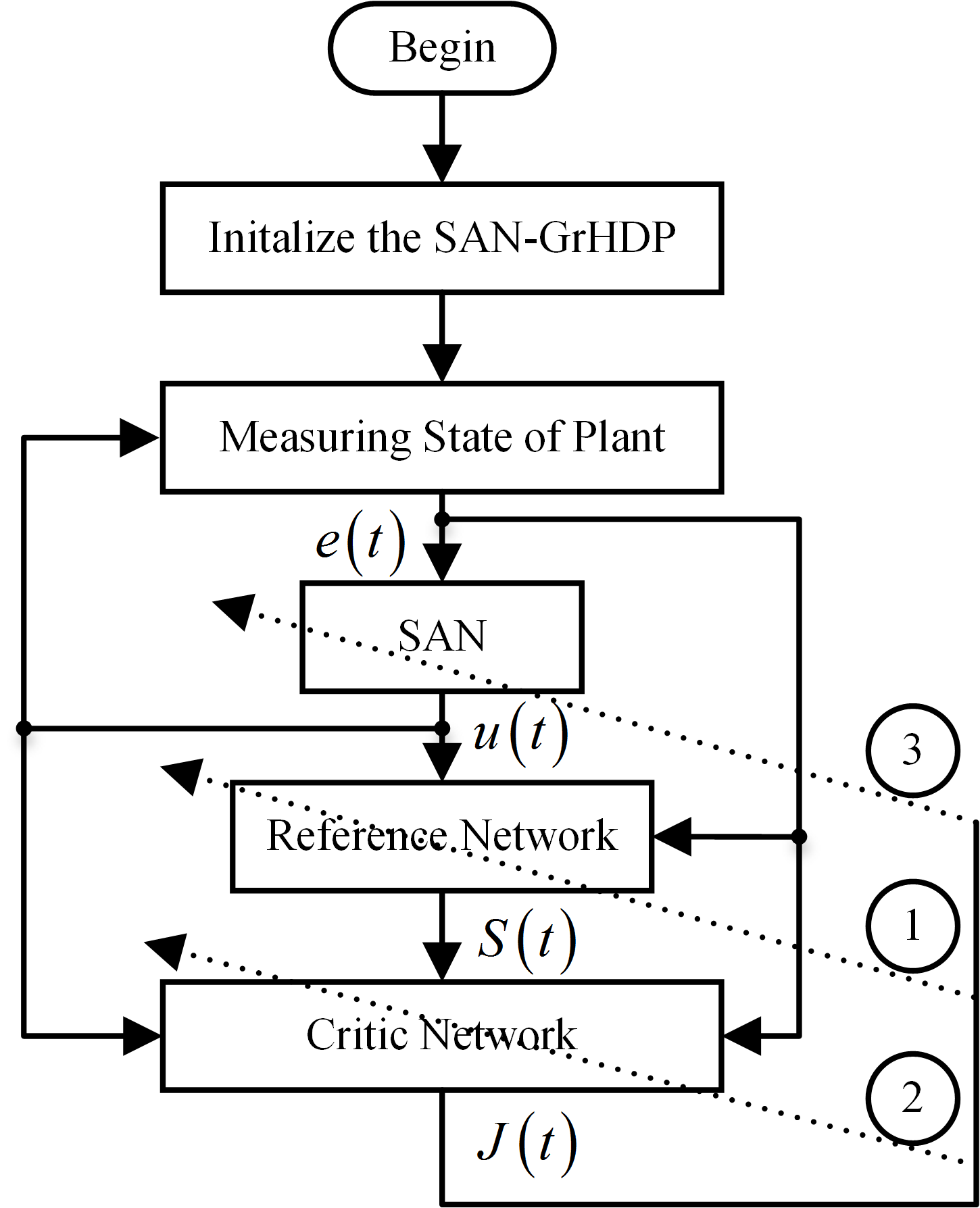
In the field of oriented control system of PMSM, speed difference is usually chosen as the input signal for the speed controller. In this SAN-GrHDP controller, previous control output is usually used as a supplementary signal input of the controller, so the controller input is of error value $e\left(t\right)$ at time t, error value $e\left(t-1\right)$ at time t − 1, error value $e\left(t-2\right)$ at time t − 2, previous control output value $u\left(t-1\right)$, and the controller output is $u\left(t\right)$. The optimization parameters of controller will be updated accordingly by online learning. The data flowchart is shown in Figure 6 and the algorithm training process is described as follows:

(1)

Initialize the various parameters of the SAN-GrHDP, such as neural network learning rate, the initial weights values of neural network, discount factor and so on.

(2)

Observe the differences of speed and obtain the control signal $u\left(t\right)$ that is q-axis current reference value for the control system of PMSM.

(3)

Calculate the internal reinforcement learning signal $S\left(t\right)$, and the value function signal $J\left(t\right)$.

(4)

Retrieve the previous time data $S\left(t-1\right)$ and $J\left(t-1\right)$, calculate the temporal difference errors and obtain the objective functions in reference network and critic network.

(5)

Update the weights values of reference network, critic network and the K value of action network (SAN).

(6)

Repeat from the second step when entering the t + 1 step.

4.3. Simulation and Experimental Results

The weights of the reference network and critic network in SAN-GrHDP approach are initialized randomly. For comparative studies, the parameters of SAN control approach are set the same as the SAN-GrHDP approach. To check the overall performance of the SAN-GrHDP control approach, simulation, and experiment on the speed control system of PMSM are carried out.

4.3.1. Simulation Results

To compare the disturbance rejection performance of both approaches, the comparative simulation of the proposed SAN-GrHDP control approach and the traditional SAN control approach are implemented on Simulink Matlab2016a (MathWorks, Natick, MA, USA). The parameters of the PMSM used in the simulation are listed in

Table 2. Parameters setting of the PMSM.

Parameter	Symbol	Value
Rated Voltage	$V$	36 V
Rated Current	$I$	4.6 A
Maximum Current	$I_{\max }$	13.8 A
Rated Power	$P$	100 W
Rated Torque	$T$	0.318 N·m
Stator Phase Resistance	$R$	0.375 Ohm
Motor Inertia	$SI$	0.0588 kg·m2·10−4
Pole Pairs	$P_n$	4 Pair
Q-axis Inductance	$L_q$	0.001 H
D-axis Inductance	$L_d$	0.001 H
Incremental Encoder Lines	$N$	2500PPR

. The parameters of both current PI are the same: the proportional coefficient is 9, the integral coefficient is 3375. The saturation limit of the q-axis reference current $i_q^{*}$ is $\pm$10 A. The initial load of PMSM is 0.2 N·m.

Figure 7 shows that simulation responses under SAN and SAN-GrHDP approaches in the presence of load torque disturbance at 1300 rpm. Figure 8 shows that simulation responses under SAN and SAN-GrHDP approaches in the presence of load torque disturbance at 800 rpm. Figure 7a shows that the SAN-GrHDP-based controller gives the same settling time with a same overshoot compared with the SAN-based controller, in the case of 1300 rpm reference speed. Figure 8a shows that the SAN-GrHDP-based controller gives the same settling time with a same overshoot compared with the SAN-based controller, in the case of 800 rpm reference speed. It can also be seen that, when a load torque 0.5 N·m is applied at 0.1 s, the SAN-GrHDP approach has less speed fluctuation than the traditional SAN approach.

Figure 7b shows that the q-axis current response under SAN and SAN-GrHDP approaches in the presence of load torque disturbance at 1300 rpm. It shows that the q-axis current $i_q$ is quite large at the moment of the start of PMSM. The $i_q^{*}$ is much less than 10 A, which is the saturation limit of the output. As the speed is steady, the actual q-axis current $i_q$ decreases down to reference q-axis current $i_q^{*}$. It can also be seen that, when a load torque 0.5 N·m is applied at 0.1 s, the actual q-axis current $i_q$ of both approaches rise quickly under the sudden load disturbance impact. However, the SAN-GrHDP approach has less current fluctuation than the traditional SAN control approach. Figure 8b shows that the q-axis current response under SAN and SAN-GrHDP approaches in the presence of load torque disturbance at 800 rpm. It can be seen from the Figure 7b and Figure 8b, when the same load torque 0.5 N·m is added suddenly at different speed, the q-axis current response at 1300 rpm is same as 800 rpm.

The evolution of the neural network parameters is presented in the SAN-GrHDP controller at 1300 rpm in Figure 7c–e. Figure 7c shows that the trajectory of the parameter K. At the load disturbance time (0.1 s), the neural network weights are adapting dramatically, which is constant with the full-size adjustments in the reinforcement signals, as shown in Figure 7d,e. The reason is that in spite of the load mutation, the system is converting according to the controller learning surroundings, so that it adapt its parameters to provide the most suitable control signal for the system again to achieve its normal working point. The evolution of the neural network parameters is presented in the SAN-GrHDP controller at 800 rpm in Figure 8c–e.

4.3.2. Experimental Results

An experimental platform for a PMSM device is built to evaluate the overall performance of the proposed SAN-GrHDP control approach. The configuration and the experimental test setup are shown in Figure 9 and Figure 10, respectively.

All the control algorithms, which include the SVPWM technique, are implemented by using this system of the floating DSP TMS320F28335 with a clock frequency of one hundred and fifty MHz, the usage of a C-language. The current-loop sampling period is 200 μs, the speed loop sampling time is ten times that of the current loop. The saturation restriction of the q-axis reference current is $\pm$10 A. The PMSM is driven by using an intelligent power module (IPM) PS21965, which is designed by the Mitsubishi Company (Tokyo, Japan). The phase currents are measured by Hall sensors, converted to voltages by sampling resistances and AD7606 converter. The rotor speed and absolute rotor position can be measured by the incremental position encoder of 2500 lines. The speed and q-axis current signals are displayed on the oscilloscope, through a DAC converter (AD5344) output.

The parameters of both current PI units are the same: the proportional coefficient is 0.2, the integral coefficient is 0.006. The parameters of SAN are as follow: ${\eta }_p=0.05$, ${\eta }_I=0.05$. The initial value of scale-up factor K = 0.01. The parameters of SAN-GrHDP are shown in Table 1, the parameters of action network are same as SAN control approach.

Figure 11 shows the experimental response curves of speed and i_q with sudden load disturbance by SAN control approach at 1300 rpm. Figure 12 shows the experimental response curves of speed and i_q with the same sudden load disturbance by SAN-GrHDP approach at 1300 rpm. From Figure 11, it can be seen that the speed of SAN approach fluctuates greatly when load is added. It can be inferred from Figure 11 that the control effect of SAN can be improved with application of the machine learning (GrHDP) to tuning the K value. The proposed control strategy can quickly stabilize the speed when load is added. Figure 13 and Figure 14 show the comparative experimental response curves with the SAN and proposed SAN-GrHDP approach at 800 rpm, respectively. The experimental results in Figure 13 and Figure 14 are similar in Figure 11 and Figure 12. From the experimental results, it can be seen that there are some differences from the results of simulation. The reason is that the PMSM model in simulation is ideal, and it has some disparities in practical application. In the process of experiment, the fluctuation error of speed is greater than the simulation result in steady state. The proposed SAN-GrHDP approach is a kind of machine learning algorithm (ADP). It can learned by itself according to the environmental characteristics. Therefore, the weights of neural networks in experiment are different from that of simulation. This is also the reason for disparities between simulation and experimental results. It is found that compared with the SAN control approach, the proposed SAN-GrHDP approach indicates a higher disturbance rejection potential, with much less speed fluctuation and shorter recovering time towards load disturbance.

5. Conclusions

In order to improve the disturbance rejection capacity of PMSM closed-loop systems, the design and implementation of a novel adaptive speed controller for a PMSM was investigated in this paper. This controller was a composite reinforcement learning control approach which combines SAN and GrHDP collectively, namely SAN-GrHDP. The proposed control approach could develop an internal reinforcement learning signal to adjust the K value of the traditional SAN control approach, whenever external parameters varies.

From our simulation and experimental results, it could be concluded that the dual closed-loop structures of PMSM under the proposed SAN-GrHDP approach had a satisfying dynamic overall performance. The composite SAN-GrHDP approach was able to achieve a fulfilling performance with speedy temporary reaction, precise disturbance rejection capacity.

Because of the uncertainty of the network weights, most articles about the ADP approach put all the emphasis on the simulation part, instead of actual applications. In this article, the traditional GrHDP approach was improved and the action network was replaced by SAN. The stability of this proposed algorithm could be improved in practical applications by using SAN. The core idea of the proposed algorithm is machine learning. At this stage, there are still some unstable situations in practical applications, such as longer training time, complex structure, and so on. However, it is promising to apply it in actual control system to solve electric engineering problems.

Finally, perspectives on future research may be listed as follows. (1) The learning rate of the neural network can be chosen in an optimal way; (2) The success rate of the algorithm should be improved; (3) A rigorous stability analysis is required to show the convergence of SAN-GrHDP approach; (4) The critic and reference neural networks should be replaced by other mathematical models; (5) Some experimental designs of internal disturbance rejection capacity (PMSM parameter variations) of proposed SAN-GrHDP approach should be discussed in detail; (6) Only one input variable (PMSM speed) is taken into consideration in the proposed scheme. Therefore, further investigation can expand it to a more generalized case of multi-variables.

References

- Calvini, M.; Carpita, M.; Formentini, A.; Marchesoni, M. PSO-Based Self-Commissioning of Electrical Motor Drives. IEEE Trans. Ind. Electron. 2015, 62, 768–776. [Google Scholar] [CrossRef]
- Li, S.; Liu, Z. Adaptive Speed Control for Permanent-Magnet Synchronous Motor System with Variations of Load Inertia. IEEE Trans. Ind. Electron. 2009, 56, 3050–3059. [Google Scholar] [CrossRef]
- Jung, J.W.; Leu, V.Q.; Do, T.D.; Kim, E.K.; Choi, H.H. Adaptive PID Speed Control Design for Permanent Magnet Synchronous Motor Drives. IEEE Trans. Power Electron. 2015, 30, 900–908. [Google Scholar] [CrossRef] [Green Version]
- Underwood, S.J.; Husain, I. Online Parameter Estimation and Adaptive Control of Permanent-Magnet Synchronous Machines. IEEE Trans. Ind. Electron. 2010, 57, 2435–2443. [Google Scholar] [CrossRef]
- Liu, J.; Li, H.; Deng, Y. Torque Ripple Minimization of PMSM Based on Robust ILC via Adaptive Sliding Mode Control. IEEE Trans. Power Electron. 2018, 33, 3655–3671. [Google Scholar] [CrossRef]
- Repecho, V.; Biel, D.; Arias, A. Fixed Switching Period Discrete-Time Sliding Mode Current Control of a PMSM. IEEE Trans. Ind. Electron. 2018, 65, 2039–2048. [Google Scholar] [CrossRef]
- Joo, K.; Park, J.; Lee, J.; Joo, K.J.; Park, J.S.; Lee, J. Study on Reduced Cost of Non-Salient Machine System Using MTPA Angle Pre-Compensation Method Based on EEMF Sensorless Control. Energies 2018, 11, 1425. [Google Scholar] [CrossRef]
- Park, J.; Wang, X.; Park, J.B.; Wang, X. Sensorless Direct Torque Control of Surface-Mounted Permanent Magnet Synchronous Motors with Nonlinear Kalman Filtering. Energies 2018, 11, 969. [Google Scholar] [CrossRef]
- Su, D.; Zhang, C.; Dong, Y.; Su, D.; Zhang, C.; Dong, Y. An Improved Continuous-Time Model Predictive Control of Permanent Magnetic Synchronous Motors for a Wide-Speed Range. Energies 2017, 10, 2051. [Google Scholar] [CrossRef]
- Yang, M.; Liu, Z.; Long, J.; Qu, W.; Xu, D.; Yang, M.; Liu, Z.; Long, J.; Qu, W.; Xu, D. An Algorithm for Online Inertia Identification and Load Torque Observation via Adaptive Kalman Observer-Recursive Least Squares. Energies 2018, 11, 778. [Google Scholar] [CrossRef]
- Sun, X.; Chen, L.; Yang, Z.; Zhu, H. Speed-Sensorless Vector Control of a Bearingless Induction Motor with Artificial Neural Network Inverse Speed Observer. IEEE/ASME Trans. Mechatron. 2013, 18, 1357–1366. [Google Scholar] [CrossRef]
- Chaoui, H.; Sicard, P. Adaptive Fuzzy Logic Control of Permanent Magnet Synchronous Machines with Nonlinear Friction. IEEE Trans. Ind. Electron. 2012, 59, 1123–1133. [Google Scholar] [CrossRef]
- Barkat, S.; Tlemçani, A.; Nouri, H. Noninteracting Adaptive Control of PMSM Using Interval Type-2 Fuzzy Logic Systems. IEEE Trans. Fuzzy Syst. 2011, 19, 925–936. [Google Scholar] [CrossRef]
- Lai, C.K.; Shyu, K.-K. A novel motor drive design for incremental motion system via sliding-mode control method. IEEE Trans. Ind. Electron. 2005, 52, 499–507. [Google Scholar] [CrossRef]
- Liu, J.; Vazquez, S.; Wu, L.; Marquez, A.; Gao, H.; Franquelo, L.G. Extended State Observer-Based Sliding-Mode Control for Three-Phase Power Converters. IEEE Trans. Ind. Electron. 2017, 64, 22–31. [Google Scholar] [CrossRef]
- Do, T.D.; Kwak, S.; Choi, H.H.; Jung, J.W. Suboptimal Control Scheme Design for Interior Permanent-Magnet Synchronous Motors: An SDRE-Based Approach. IEEE Trans. Power Electron. 2014, 29, 3020–3031. [Google Scholar] [CrossRef]
- Sun, X.; Shi, Z.; Chen, L.; Yang, Z. Internal Model Control for a Bearingless Permanent Magnet Synchronous Motor Based on Inverse System Method. IEEE Trans. Energy Convers. 2016, 31, 1539–1548. [Google Scholar] [CrossRef]
- Sun, X.; Chen, L.; Jiang, H.; Yang, Z.; Chen, J.; Zhang, W. High-Performance Control for a Bearingless Permanent-Magnet Synchronous Motor Using Neural Network Inverse Scheme Plus Internal Model Controllers. IEEE Trans. Ind. Electron. 2016, 63, 3479–3488. [Google Scholar] [CrossRef]
- Si, J.; Wang, Y.-T. Online learning control by association and reinforcement. IEEE Trans. Neural Netw. 2001, 12, 264–276. [Google Scholar] [CrossRef] [PubMed] [Green Version]
- Prokhorov, D.V.; Wunsch, D.C. Adaptive critic designs. IEEE Trans. Neural Netw. 1997, 8, 997–1007. [Google Scholar] [CrossRef] [PubMed] [Green Version]
- He, H.; Ni, Z.; Fu, J. A three-network architecture for on-line learning and optimization based on adaptive dynamic programming. Neurocomputing 2012, 78, 3–13. [Google Scholar] [CrossRef]
- He, H. Adaptive Dynamic Programming for Machine Intelligence. In Self-Adaptive Systems for Machine Intelligence; John Wiley & Sons, Inc.: Hoboken, NJ, USA, 2011; pp. 140–164. ISBN 978-1-118-02560-4. [Google Scholar]
- Tang, Y.; He, H.; Wen, J.; Liu, J. Power System Stability Control for a Wind Farm Based on Adaptive Dynamic Programming. IEEE Trans. Smart Grid 2015, 6, 166–177. [Google Scholar] [CrossRef]
- Tang, Y.; Mu, C.; He, H. SMES-Based Damping Controller Design Using Fuzzy-GrHDP Considering Transmission Delay. IEEE Trans. Appl. Supercond. 2016, 26, 1–6. [Google Scholar] [CrossRef]
- Tang, Y.; Yang, J.; Yan, J.; He, H. Intelligent load frequency controller using GrADP for island smart grid with electric vehicles and renewable resources. Neurocomputing 2015, 170, 406–416. [Google Scholar] [CrossRef] [Green Version]
- Mishra, S. Neural-network-based adaptive UPFC for improving transient stability performance of power system. IEEE Trans. Neural Netw. 2006, 17, 461–470. [Google Scholar] [CrossRef] [PubMed]
- Cao, H.; Li, X. Thermal Management-Oriented Multivariable Robust Control of a kW-Scale Solid Oxide Fuel Cell Stand-Alone System. IEEE Trans. Energy Convers. 2016, 31, 596–605. [Google Scholar] [CrossRef]
- Butt, C.B.; Rahman, M.A. Untrained Artificial Neuron-Based Speed Control of Interior Permanent-Magnet Motor Drives Over Extended Operating Speed Range. IEEE Trans. Ind. Appl. 2013, 49, 1146–1153. [Google Scholar] [CrossRef]
- Ma, G.Y.; Chen, W.Y.; Cui, F.; Zhang, W.P.; Wu, X.S. Adaptive levitation control using single neuron for micromachined electrostatically suspended gyroscope. Electron. Lett. 2010, 46, 406–408. [Google Scholar] [CrossRef]
- Zhong, X.; Ni, Z.; He, H. A Theoretical Foundation of Goal Representation Heuristic Dynamic Programming. IEEE Trans. Neural Netw. Learn. Syst. 2016, 27, 2513–2525. [Google Scholar] [CrossRef] [PubMed]
- Liu, D.; Zhang, Y.; Zhang, H. A self-learning call admission control scheme for CDMA cellular networks. IEEE Trans. Neural Netw. 2005, 16, 1219–1228. [Google Scholar] [CrossRef] [PubMed]
- Lin, W.-S.; Yang, P.-C. Adaptive critic motion control design of autonomous wheeled mobile robot by dual heuristic programming. Automatica 2008, 44, 2716–2723. [Google Scholar] [CrossRef]
- Liu, Y.J.; Gao, Y.; Tong, S.; Li, Y. Fuzzy Approximation-Based Adaptive Backstepping Optimal Control for a Class of Nonlinear Discrete-Time Systems with Dead-Zone. IEEE Trans. Fuzzy Syst. 2016, 24, 16–28. [Google Scholar] [CrossRef]
- Nguyen, T.L. Adaptive dynamic programming-based design of integrated neural network structure for cooperative control of multiple MIMO nonlinear systems. Neurocomputing 2017, 237, 12–24. [Google Scholar] [CrossRef]
- Mu, C.; Ni, Z.; Sun, C.; He, H. Data-Driven Tracking Control with Adaptive Dynamic Programming for a Class of Continuous-Time Nonlinear Systems. IEEE Trans. Cybern. 2017, 47, 1460–1470. [Google Scholar] [CrossRef] [PubMed]
- Tang, Y.; He, H.; Ni, Z.; Zhong, X.; Zhao, D.; Xu, X. Fuzzy-Based Goal Representation Adaptive Dynamic Programming. IEEE Trans. Fuzzy Syst. 2016, 24, 1159–1175. [Google Scholar] [CrossRef]
- Li, S.; Zhou, M.; Yu, X. Design and Implementation of Terminal Sliding Mode Control Method for PMSM Speed Regulation System. IEEE Trans. Ind. Inf. 2013, 9, 1879–1891. [Google Scholar] [CrossRef]
- Krause, P.C.; Wasynczuk, O.; Sudhoff, S.D. Analysis of Electric Machinery; Wiley-IEEE Press: New York, NY, USA, 1995; ISBN 978-0-7803-1101-5. [Google Scholar]
- Ni, Z.; He, H.; Wen, J.; Xu, X. Goal Representation Heuristic Dynamic Programming on Maze Navigation. IEEE Trans. Neural Netw. Learn. Syst. 2013, 24, 2038–2050. [Google Scholar] [CrossRef] [PubMed]
- Shen, Y.; Chen, W.; Yao, W.; Liao, S.; Wen, J. Supplementary Damping Control of VSC-HVDC for Interarea Oscillation Using Goal Representation Heuristic Dynamic Programming. In Proceedings of the 12th IET International Conference on AC and DC Power Transmission (ACDC 2016), Beijing, China, 28–29 May 2016. [Google Scholar] [CrossRef]
Figure 1.
The field oriented control (FOC) diagram of permanent magnet synchronous motor (PMSM) system by id = 0 control approach.
Figure 2.
Schematic diagram of FOC by proposed single artificial neuron goal representation heuristic dynamic programming (SAN-GrHDP).
Figure 3.
Schematic diagram of the reference network.
Figure 4.
Schematic diagram of the critic network.
Figure 5.
Schematic diagram of the action network (SAN).
Figure 6.
Flowchart of the SAN-GrHDP procedure.
Figure 7.
Simulation responses under SAN and SAN-GrHDP approaches in the presence of load torque disturbance at 1300 rpm. (a) Speed. (b) . (c) K value of the SAN-GrHDP approach. (d) S value of the SAN-GrHDP approach. (e) J value of the SAN-GrHDP approach.
Figure 8.
Simulation responses under SAN and SAN-GrHDP approaches in the presence of load torque disturbance at 800 rpm. (a) Speed. (b) . (c) K value of the SAN-GrHDP approach. (d) S value of the SAN-GrHDP approach. (e) J value of the SAN-GrHDP approach.
Figure 9.
Configuration of the experimental system.
Figure 10.
Experimental test setup.
Figure 11.
Experimental responses under SAN in the presence of load torque disturbance at 1300 rpm. (a) Speed; and (b) .
Figure 12.
Experimental responses under SAN-GrHDP in the presence of load torque disturbance at 1300 rpm. (a) Speed; and (b) .
Figure 13.
Experimental responses under SAN in the presence of load torque disturbance at 800 rpm. (a) Speed; and (b) .
Figure 14.
Experimental responses under SAN-GrHDP in the presence of load torque disturbance at 800 rpm. (a) Speed; and (b) .