How Elastic Demand Affects Bidding Strategy in Electricity Market: An Auction Approach

1
Economics and Management School, Wuhan University, Wuhan 430072, China
2
School of Economics, Wuhan University of Technology, Wuhan 430070, China
*
Author to whom correspondence should be addressed.
Energies 2019, 12(1), 9; https://doi.org/10.3390/en12010009
Submission received: 20 November 2018
/
Revised: 12 December 2018
/
Accepted: 17 December 2018
/
Published: 21 December 2018
(This article belongs to the Section F: Electrical Engineering)
Abstract
:The deepening of electricity reform results in increasingly frequent auctions and the surge of generators, making it difficult to analyze generators’ behaviors. With the difficulties to find analytical market equilibriums, approximate equilibriums were obtained instead in previous studies by market simulations, where in some cases the results are strictly bound to the initial estimations and the results are chaotic. In this paper, a multi-unit power bidding model is proposed to reveal the bidding mechanism under clearing pricing rules by employing an auction approach, for which initial estimations are non-essential. Normalized bidding price is introduced to construct generators’ price-related bidding strategy. Nash equilibriums are derived depending on the marginal cost and the winning probability which are computed from bidding quantity, transmission cost and demand distribution. Furthermore, we propose a comparative analysis to explore the impact of uncertain elastic demand on the performance of the electricity market. The result indicates that, there exists market power among generators, which lead to social welfare decreases even under competitive conditions but elastic demand is an effective way to restrain generators’ market power. The feasibility of the models is verified by a case study. Our work provides decision support for generators and a direction for improving market efficiency.
1. Introduction
Following the attempts in the U.S., Britain, Australia and Russia, many other countries are deepening the massive reforms of the electricity market [1]. Since the significant document ‘Several Opinions on Further Deepening the Reform of Electric Power System (No.9 document)’ was issued in March 2015, China’s electric power market is gradually introducing competition and establishing a market-oriented power trading platform, allowing new kinds of participants to emerge [2]. Consumers exhibit higher sensitivity for price and market demand varies from fixed demand to uncertain elastic demand with the participation of large bargaining customers [3]. On the supply side, many small and medium-sized electricity generators are involved in the competition, entailing fierce competitions and frequent auctions among them [4]. Governments in various countries, such as China, England, Spain and others perform wholesale electricity transactions via Uniform Clearing Price (UCP) auction mechanisms to balance the supply and demand and improve the economic efficiency [5,6,7]. Therefore, with the increasing open electricity market, it is crucial to effectively analyze the behavior of electricity generators and seek market equilibrium prices accurately.
To study this related issue, many scholars focus on modeling and analyzing generators’ behavior patterns in a competitive electricity market since 2000 [8,9,10,11,12,13,14,15,16,17,18,19]. Due to the difficulty in obtaining the analytical market equilibrium, the approximate market equilibriums concerning generators’ behaviors are sought by market simulations, such as agent-based simulation [9,10], evolutionary simulation [11], and hybrid iterative simulation [12,13]. For instance, Wang et al. [11] proposed an evolutionary game approach to analyze the bidding process based on price-responsive demand. The generators update their beliefs of opponents’ strategies and optimize their bid based on the updated information. By repeated adaptive learning, the electricity market eventually converges to the equilibrium, where no players can increase their profit by changing their strategies unilaterally. However, market simulations do not provide systematic approaches to building bidding strategies [16]. In addition, market simulations have become a complex process to seek market equilibrium in the frequent large-scale auction due to the surge of participants and the increase of market uncertainty. Some experiments indicated that the equilibrium may not be found and the results were directly related to initial estimations in some cases [11,17]. In other words, most iterative algorithms are strictly connected to the initial estimations since the results would be chaotic if the initial estimations were improper.
To fill these gaps, auction models provide analytical rationale and explanation about how market equilibrium can be decided via strategic bidding behavior. Unlike simulation technology which emphasizes learning processes, auction models solve the optimal bidding problem by considering the interaction of generators, and achieve the economic equilibrium of power market through a Nash equilibrium. Auction approaches avoid initial estimations and the time limit of simulation technology. The existing researches related to bidding strategies by auction models, always concentrate on bidding behaviors based on the assumption that demand is fixed and inelastic [20,21,22,23,24,25,26,27,28], which does not always hold in practice, especially in the market-oriented market. For instance, Hao [20] modeled bidding behaviors and assumed that demand, which is known to all electricity generators, was fixed. The results showed that those bidders would exert their market power to bid below their marginal cost so as maximize the expected profits. Similarly, Li and Shahidehpour [23] proposed a novel bidding model to discuss the Nash equilibrium in the electricity market. Based on this proposed model, Banaei et al. [24] discussed wind generator’s bidding strategy and Rahimiyan and Baringo [25] researched ISO’s scheduling problem. However, the literatures on the key role of the market demand in the bidding strategy are insufficient. Characteristics of electricity demand, a key factor to strategic behaviors, such as seasonality, time-fluctuation and price-responsiveness, has received less attention [13]. Compared to other commodities, the demand elasticity of electricity is low, but even a low demand elasticity can result in a noticeable difference of the market performance [18].
Given all of the above, this paper applies auction theory to model the generators’ optimal bidding strategy based on the uncertain elastic demand and to explore the Nash equilibrium under clearing pricing rules, for which initial estimations are non-essential. In UCP auction, all participants submit their bids to Independent System Operators (ISOs) simultaneously and independently according to their demand information and expected profit. The lower price participants are assigned with the demand quantity first and the Market Clearing Prices (MCPs) are the highest prices that produce demand. Due to the information asymmetry, the bidding process is a non-cooperative oligopoly game with incomplete information. Anticipated MCPs, transaction cost, cost distribution of opponents (public information) and own true marginal cost (private information), are all considered in our model. With efforts to introduce transmission cost into the bidding strategy, normalized bidding price is applied innovatively. It ensures that the generators providing a large quantity are more likely to win the auction when bidding prices are equal. Results show that generators would exert market power to bid higher than their marginal cost in order to maximize expected profits. The optimal bidding price is the true marginal cost plus the winning probability, which is computed from bidding quantity, transmission cost and market demand distribution. Our work contributes game theoretic models to the auction theory literature and generates novel insights for generators seeking profits.
The intended contributions of this paper are listed as follows: (1) to propose a simple and effective auction model that provides a systematic approach to building bidding strategies under the uncertain elastic demand. A unique analytical Nash equilibrium is obtained, which solves the time limit and initial estimations problem; (2) to provide a comparative analysis to assess the impact of the demand elasticity on the performance of the electricity market (UCP auction VS. complete competition VS. fixed demand auction), which is rare to conventional wisdoms; (3) to disclose the market power among generators under competitive conditions and prove that elasticity of the market demand is an effective way to restrain generators’ market power.
The rest of this paper proceeds as follows: in Section 2, the model is established and the optimal bidding strategies are presented. In Section 3, we discuss how uncertain price-responsive demand influences the performance of the electricity market, and case studies are undertaken to verify the proposed model. The conclusions are given in Section 4.
2. The Basic Model
2.1. Electricity Market and MCP
In an electricity market game, due to the information asymmetry that exists in the bidding process, such as opponents’ marginal cost and opponents’ bidding behavior, the bidding process can be described as an asymmetric information game of divisible object. We suppose a model for generators i (i = 1, 2, …, m) with different marginal costs, which compete to sell homogenous goods to the market. In period , the sequence of events in classical UCP can be seen in the following paragraphs [29,30]:
- (1)
- The auctioneer releases market information according to market operation rules, including the demand information and the bidding history of participant generators.
- (2)
- Each generator simultaneously and independently submits a bidding price at which it is willing to supply its maximum production up to quantity .
- (3)
- These bids are ranked in terms of the bidding price .
- (4)
- The lower price generator is assigned with the demand quantity first. If his quantity cannot satisfy the demand, the higher price bidders produce the residual demand. If the bidders submit equal bids, then they split the market equally.
- (5)
- MCP is the highest price that produces the demand. Generators would not participate in a bid if their bidding prices were higher than the MCP.
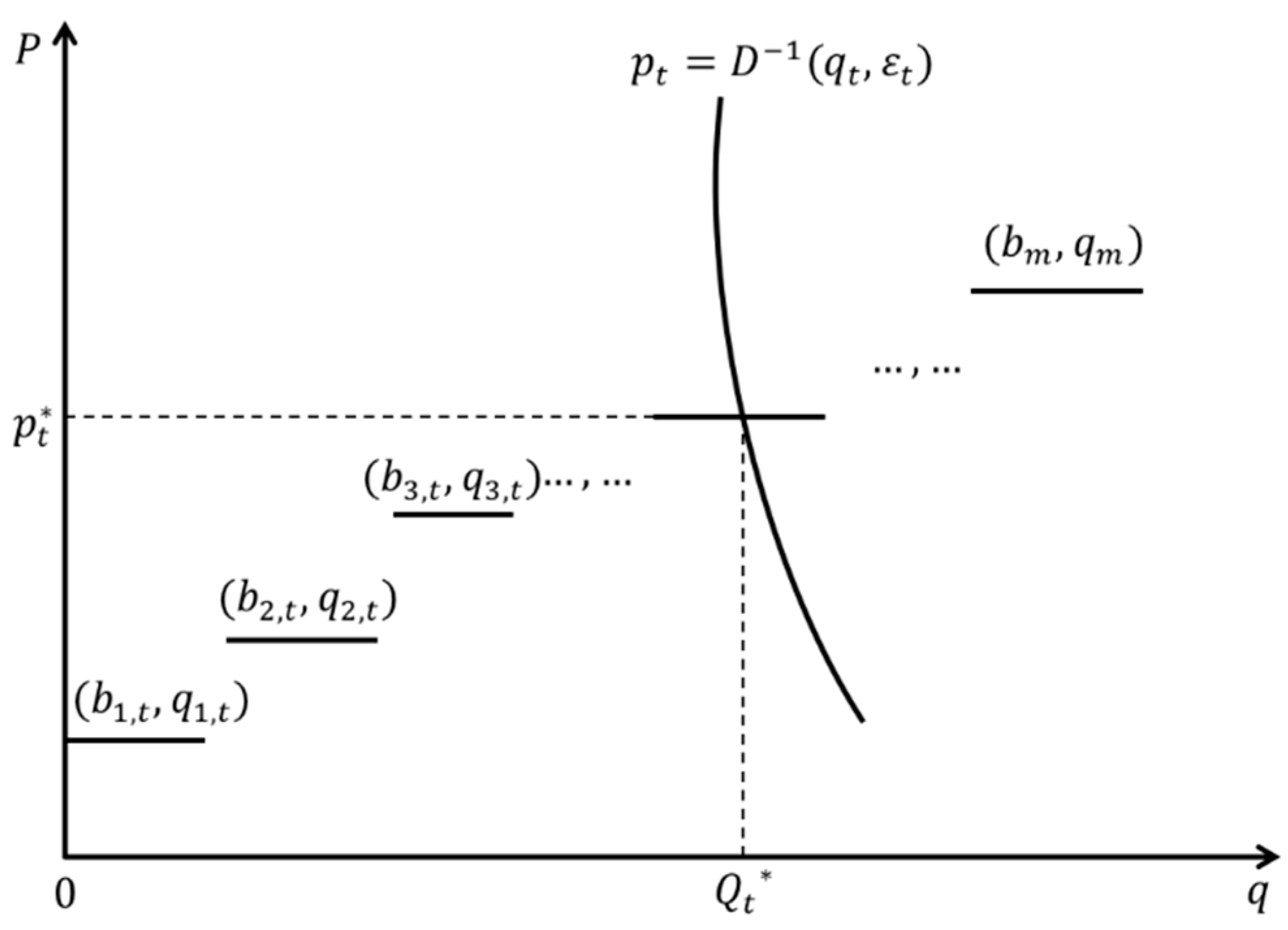
The bidding curves are composed of all generators’ pair of quantity- price (Figure 1), The day-ahead market demand function in period is represented by , which is a function of random shock and market price . It is assumed to satisfy the following standard assumptions: is strictly increases in , and strictly decreases and concaves in . Demand shock is a random variable with a differentiable cumulative distribution function and a continuous density function . The bidding curves are composed of all generators’ pairs of quantity-price (Figure 1).
As shown in Figure 2, from the perspective of the generators, the decision-making process can be divided into five steps in the specific process of the UCP auction:
- Step 1:
- Information acquisition. The generators get related information from the auctioneer, including the demand information and the bidding history of participant generators.
- Step 2:
- Price normalization. The generators normalize the bidding prices integrating the transaction cost.
- Step 3:
- Winning probability. The generators calculate the winning probability based on private costs.
- Step 4:
- Optimal strategy. The generators submit the optimal bids.
- Step 5:
- Nash equilibrium. Market equilibrium is the intersection of the demand function and the bidding curves.
The generator ’s truly variable marginal cost is considered as a constant, which is private information only precisely known to itself and independent of each other. The generator can estimate others’ marginal cost by probability distribution, which can be described with density function and cumulative distribution function . In practical, the cost can be estimated from manufacturers or from market reports [31].
With the progress of the electricity market liberalization, the ISO is just a network provider who has withdrawn from power trading. The generators, on the other hand, need to pay wheeling costs and auxiliary service costs, which account for a large proportion of the whole electricity cost [28,32]. Therefore, in addition to the cost of generating electricity, wheeling cost and auxiliary service cost are also indispensable costs to generators and consider as the transmission cost in this paper. Generally, for a certain quantity of electricity, transaction costs will increase as the number of transactions increases. Therefore a standardized bidding price is introduced into the mechanism to ensure that generators with a large supply quantity will be more likely to win the auction when the bidding prices are equal.
Suppose the transaction cost function is , where , is the bidding quantity. Therefore denotes the transaction cost of the generator when one unit quantity is traded. If the generator bidding unit with bidding price and wins the auction, his ex post profit is . Generator can be viewed as virtual generators who bid one unit with the same virtual bidding price . So each generator’s ex post profit is . Because the final profit is the same, according to the principle of equivalent profit, the relationship between the actual bidding price and the virtual bidding price is shown by Equation (1):
By normalized bidding price, we convert generators into virtual generators, each virtual generator bidding 1 unit quantity to the auctioneer. So generator is converted to virtual generators, whose bidding information is . In the operation of actual electricity market, a generator does not change its production schedule frequently, because it leads to excessive operational inefficiencies for the generator [5]. Therefore, although the generation quantity affects the bid price, it is not a decision variable.
As mentioned above from the UCP rules, if the virtual generator’ bidding price is lower than the MCP , he produces one unit as his bid quantity. If his bidding price is equal to the MCP, he produces the residual demand . However, the bidding prices of different virtual generators may be the same. In this case, if the bidding price is below the MCP , the distribution rules do not change and all the virtual generators produce one unit as their bid quantity. If the bidding price is equal to the MCP , the distribution rules are different. Each generator with the same bidding price produces the residual demand equal to , denoting the quantity of bidders with the same bidding price. Since we assume that the cost distribution of the generators follows a continuous distribution, the probability that generators with the same bids (the same private cost) is 0, that is . The following work is to solve the virtual optimal bidding price .
2.2. Winning Probabilities
When all generators participate in a bidding game, there exist three type of generators: those winning in the margin, who bid the same as MCP; those winning below, who bid below the MCP; and those losing the game, who bid above the MCP, and the probabilities of the three outcomes are important for deriving the bidding strategy [20]. Assume that the probability of generator winning the game by bidding below the MCP is , for those winning in the margin is , and those losing the game is .
Suppose represents the MCP in period , there are generators winning the game, and represents the integer part of . If generator wins the game in the margin, the generators whose bidding price are lower than will be assigned first, and generator produces the residual demand at the MCP equal to , which is smaller than one unit. If generator wins the game by bidding below the MCP, he will be assigned first, producing one unit as his bid quantity. The probability of generator winning the game is not only related to his own strategic choice of , but related to the market demand and cost distribution of participants:
In the formula, represents the probability of the generator winning in the margin, and describes the probability of generators whose bidding prices are less than that of generator . represents the probability of generator winning below the MCP and describes the cumulative probability of at most generators’ bidding prices that are less than the price of generator .
In period , given any of other generators, each generator chooses its bid price that achieves its ex post maximum expected profit with respect to period- day-ahead demand. By doing so, the generator achieves its maximum expected profit by choosing that satisfies the following:
For any realization of bid price and random shock :
Here, is generator ’s expected profit at MCP . For example, given a random shock , if the generator ’s expected profit by choosing price is higher than that by choosing any other price set , then is an equilibrium. The formal definition of such an equilibrium is as follows.
Definition 1.
For any given other profile of bid price,is called ‘period-bid price equilibrium’ or ‘period-equilibrium’ ifsatisfies Equation (4) for.
By Equation (4), demand uncertainty is one of the major factors that put MCP at risk. In our analysis, we study an equilibrium in which the same-cost generators have the same strategies behavior. Given demand random , MCP and other generators’ strategies , generator ’s expected profit Equation (4) in period is equivalent to:
2.3. The Optimal Bidding Strategy of the Generators
In this section, we begin our analysis by characterizing generators’ equilibrium strategies. Recall Equation (5), to maximize Equation (5) for any and , generator must choose a bid price inducing a MCP that maximizes expected profit Equation (6):
is generator ’s expected profit. Note that , that is, the total demand is equal to the sum of all the bid quantities below the MCP. With such bid behaviors, generator will achieve the maximum expected profit in period if it observes the random shock after its decision in period . Then, the optimal bid price that maximizes excepted profit satisfies the following first-order condition:
Note that and the fact that private cost and random shock are independent of each other. Applied the formula of inverse function differentiation, let to rewrite Equation (7) as:
Generator ’s optimal bidding strategy satisfies the ordinary differential equation Equation (8) in interval and the boundary conditions , where the generators with the highest cost cannot bid higher than the price ceiling . Therefore, Equation (8) has a unique solution. That is to say, a generator with marginal cost has one and only one optimal bidding strategy , which maximizes its expected profit. So we obtain Proposition 1.
Proposition 1.
There exists a unique Nash equilibriumthat satisfies Equation (4) and the optimal bidding pricesatisfies Equation (8).
Integrating Equation (8) from to yields the following:
We know the fact that the probability of winning in or below the margin is 0 for the bidder with highest cost :
Considering the boundary condition and collecting Equation (9) as canonical forms, we obtain the following formal result from Equations (9) and (10):
represents the general bidding strategy given an estimate of the expected MCP . This result shows that a bidder’s optimal bid is determined by three components: its real marginal cost of production , make-up of the probability of winning below or in the margin , and the gap between the marginal cost and the expected MCP . According to Equation (11), the optimal bid price is related the expected MCP . In practical, a generator who follows this strategy exposes himself to additional risks if the expected (ex-ante) winning price is very different from the actual (ex-post) winning price. In 2000, Hao [20]’s study demonstrated that this risk can be mitigated when all bidders acted as if they were in the margin, that is, with , the expected profit to generator is no worse off than that in the best situation in which the ex post winning price is accurately estimated.
Recall the notation from previous analysis, and to state Proposition 2, we need to introduce the following notation:
represents period- day-ahead minimum demand shock that results in MCP equal to 0 when each generator’s bid quantity is . Then, from Equations (11) and (12), we identify generator ’s optimal bidding price in period :
Proposition 2.
In any period, generators’ optimal strategies are as follows:
- (1)
- For, each generatorcommits a production schedule, that satisfies Equations (1) and (13).
- (2)
- Period-day-ahead demand shockis realized and day-ahead MCPis determined. Production and profits are fulfilled in period.
Proposition 2 is remarkably simple yet significant. It leads to the optimal bidding strategy of the generators at each period. Equation (13) shows that the optimal bidding price of the generator is equal to his cost plus a make-up of winning probability that is computed from the bidding quantity, transmission cost and demand distribution. In addition, unlike a fixed demand auction which allocates the same quantity to the generators who win the auction, elastic demand auction has a different way to allocate quantity. Specifically, for a generator whose bidding price is equal to the MCP, the ISOs only allocates the residual demand to them, which gives them an incentive to lower their bidding price. Moreover, for the generators whose bidding price is below the MCP, the higher the MCP is, the higher the expected profits they have, while their bidding price will not affect the MCP. On the other hand, for generators whose bidding price is equal to the MCP, bidding price not only affects the MCP, but also affects his assigned quantity. Therefore, these generators need to find a balance between the bidding price and the allocated quantity. Compared to inelastic demand, uncertain elastic demand market has an incentive to reduce generators’ bidding price (restrain the market power of generators), which can also be confirmed in the numerical examples. None of them has the motivation to deviate from the optimal strategic from Proposition 2.
3. Numerical Examples
3.1. Generators’ Optimal Bidding Strategy with Uniform Cost Distribution
Numerical examples are presented to demonstrate applications and salient features of our results in the electricity market. For the ease of exposition, hereafter, we consider a linear demand function where and are constants. represents the demand scenario and represents the demand elasticity. All problem parameters introduced in this section are general knowledge to all firms. Table 1 shows the transaction cost function , with the higher trading quantity causing the higher transaction cost .
Table 2 shows the results of a case where five generators participate in the bidding game based on the demand function . The private cost of each generator is a uniform distribution of per MWh. We randomly select five numbers between to represent five generators’ true cost, which is private information only precisely known to themself. Demand shock is a random variable with uniform distribution between intervals [−1, 1]. Observing Table 2, the higher the private true cost , the higher the optimal bidding price , which is similar to inelastic demand. The optimal bidding price consists of the cost and the probability of winning the game ().
3.2. Impact of Demand Scenario on Generators’ Optimal Bidding Behaviors
Demand is one of the major factors that we consider affect strategic behaviors in the electricity market. In practice, electricity demand is price-responsive, although the demand slope is fixed and does not change frequently, but demand scenario is seasonal and time-varying. So in this section, we study the influence of demand scenario on bidding strategy. Similarly, we compute the optimal bidding strategies for each generators according to Proposition 2 and the results can be seem based on different demand scenario as Table 3 (3.5 to 6.5).
It can be seen from Table 3 that the optimal bid price increases when the demand scenario increases. From the microeconomic view, the increase in demand scenario will lead to higher MCP and more clearing quantity. When demand scenario varies from 4.5 to 5.5, the MCP increases from 1.37 to 1.5615 (if ), and the total clearing quantity increases from 3.1850 to 4.7192. From a macroeconomic perspective, due to the demand information released ahead of bid auction, high demand scenario increases the expectations of generators. In other words, if the demand curve moves to right, the bidding curve will move up.
3.3. Market Power to Derive Electricity Prices and Social Welfare
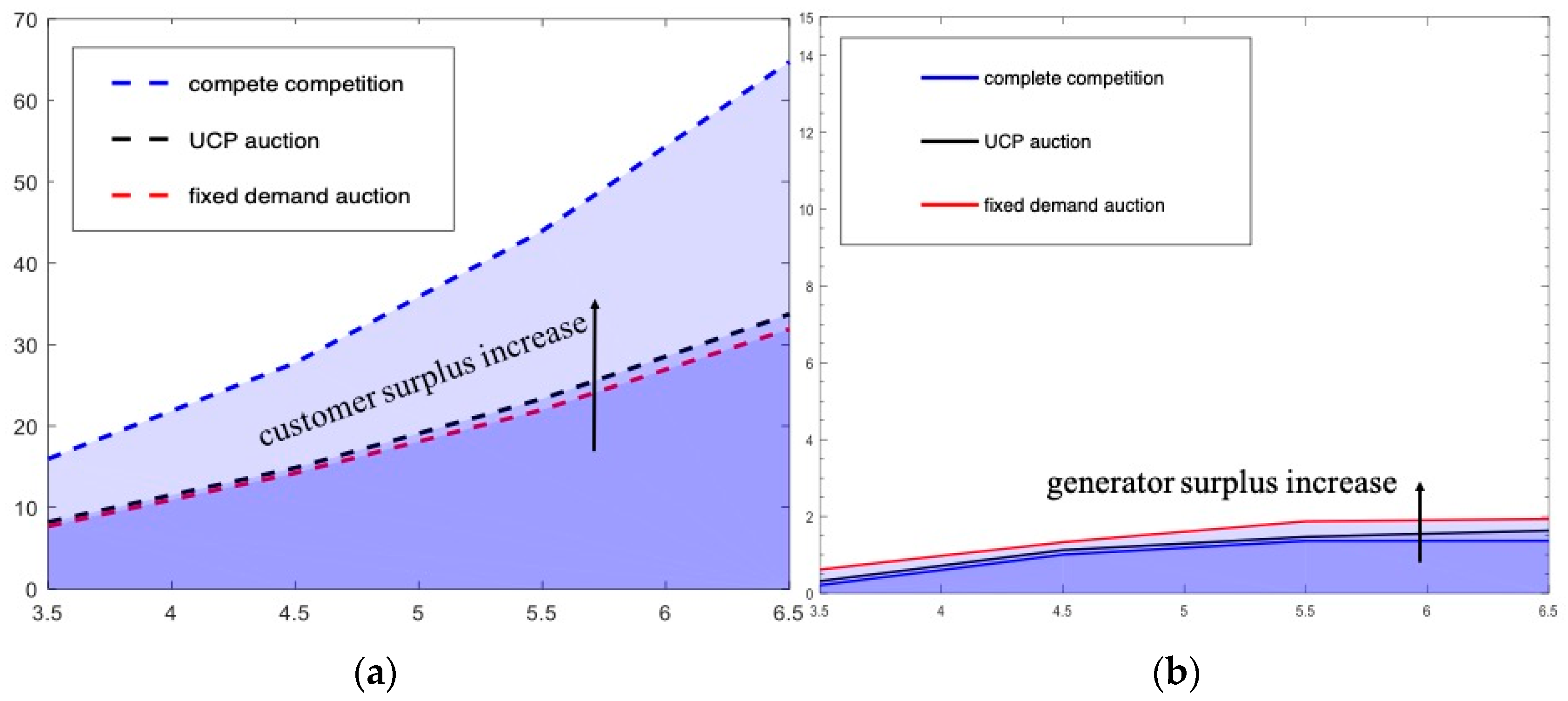
This section compares the social welfare under three market structures: UCP auction, complete competition and fixed demand auction. Supposed is the quantity actually assigned to generator in period , according to the definition in microeconomics, the total social welfare is defined as the sum of the generators surplus and the consumer surplus . Therefore, the total social welfare is as follows:
Firstly, we assume a basic scenario of complete information competition. In complete competition market, each generator offers a bidding price to the auctioneer, and MCP is the highest price that produces the demand . The generators would not participate in a bid if their bids were higher than the MCP. In this case, there is no information asymmetry and all participants know the true cost of each generator. Therefore, each generator adopts cost bidding strategy, that is . According to the allocation rules, the MCP can be calculated by the optimal strategy of the generators and the market demand conditions . Then we obtain the consumer surplus (The blue dotted line in Figure 3a) and the generators surplus (the blue solid line in Figure 3b) under complete information competition by Equation (14).
Then, we assume a fixed demand auction scenario (Hao’s research [20]). In the fixed demand auction, demand is an inelastic fixed variable and represented by . The only difference between the fixed demand auction and UCP auction is the allocation of marginal winners. In the fixed demand auction, as long as the generator wins the auction, he always has one unit of electricity allocation, that is . But in UCP auction, generators who win the auction in the margin has less than one unit of electricity allocation, that is . By substituting in Proposition 2, we can obtain:
denotes the optimal bidding strategy of generator under the fixed demand auction. Similarly, according to the allocation rules, the MCP of the fixed demand auction can be calculated by the optimal strategy of the generators and the market demand conditions . Then we can obtain the consumer surplus (the red dotted line in Figure 3a) and the generators surplus (the red solid line in Figure 3b) under the fixed demand auction by Equation (14).
Proposition 3.
Even under competitive conditions (UCP auction), there exists market power among generators. But price-responsive market demand is an effective way to restrain generators’ market power compared to inelastic market demand.
It can be seen intuitively that complete competition is a very beneficial structure for social welfare compared to UCP auction. On the one hand, complete competition brings more consumer surplus which increases as the demand scenario increases. On the other hand, although generators surplus loss will be caused by complete competition, this loss is a drop in the bucket compared to customer surplus increases. However, due to the characteristics such as asymmetric information, transmission constraints and oligopoly structure, the electricity market behaves more like an oligopoly market. Complete competition is not appropriate in the electricity market. But this comparison shows clearly that even under competitive conditions (UCP auction), there exists market power among generators.
Then, we compare our UCP auction with Hao’s fixed demand auction [20]. As shown in Figure 3, the impact of demand on social welfare is huge. Compared to fixed demand, there are more consumer surplus and more social welfare based on price-responsive demand, and this phenomenon is more evident as demand grows. For example, when demand scenario , generator surplus equals 0.9806 based on elastic demand and equals 3.113 based on fixed demand. Moreover, market price declines definitely increase consumer surplus. When demand scenario , customer surplus equals 18.1 based on elastic demand and equals 7.2771 based on fixed demand. Therefore, elasticity of demand is an effective means to restrain the market power of generators. This conclusion is similar to the results in Ruddell’s research [26], who indicated that price-responsive demands are realized to efficiently exploit the available electricity resources.
4. Conclusions
The openness of the electricity market results in generators facing fierce competition and frequent auctions and consumers exhibiting higher price sensitivity. However, due to the surge of generators and the increasingly frequent auctions, market equilibrium is difficult to pursue through market simulations and the result would be chaos if the initial estimations were not correct. Besides, seasonality, time-fluctuation and price-responsiveness of day-ahead demand, the major factors that affect strategic behaviors, have received less attention. Given this, based on the uncertain price-responsive demand, an auction model is developed to analyze asymmetric companies’ bidding strategies, in which initial estimations are not necessary. We derived the unique Nash equilibrium under clearing pricing rule by introducing normalized bidding price into bidding strategy. In particular, we take into account the effect of the demand on the generators’ bidding behavior and numerical examples are provided to show the applicability of the proposed approach.
Our results indicate that, with a UCP auction, the optimal bidding price satisfies Proposition 2, which depends on the true private cost and the winning probability calculated from bidding quantity, transmission cost and demand random. The higher the true cost, the higher the optimal bidding price. Besides, this paper compares social welfare under three market structures: UCP auction, complete competition and the fixed demand auction. This comparison shows clearly that even under competitive conditions (UCP auction), there exists market power among generators. In addition, we show that price-responsive market demand is a more effective way to restrain generators market power than inelastic market demand. The conclusion reached coincides with Ruddell’s research [26].
In addition, our paper has some limitations in. Although we have obtained the optimal strategy of the generators, we assume that the cost distribution of all generators is the same in order to obtain an analyzable Nash equilibrium, which is a relatively strong hypothesis. This hypothesis can be extended in several directions in future work. Future work includes researching the bidding strategy under different sources of power generation and designing an effective auction mechanism to monitor market power.
Author Contributions
Conceptualization, D.F. and Q.Y.; Methodology, Q.R.; Software, Q.R.; Validation, Q.Y.; Formal Analysis, D.F.; Investigation, D.F.; Resources, Q.Y.; Writing-Original Draft Preparation, D.F.; Writing-Review & Editing, Q.Y.; Supervision, D.F.; Project Administration, Q.R.; Funding Acquisition, D.F. and Q.Y.
Funding
This research was financially supported by the National Natural Science Foundation of China (Grant No. 71725007,71673210, 91647119,71774128).
Acknowledgments
The authors would like to thank the funded project for providing material for this research. We would also like to thank editor and reviewers very much for the valuable comments in developing this article.
Conflicts of Interest
The authors declare no conflict of interest.
References
- Gountis, V.P.; Bakirtzis, A.G. Bidding strategies for electricity producers in a competitive electricity marketplace. IEEE Trans. Power Syst. 2004, 19, 356–365. [Google Scholar] [CrossRef]
- The State Council. Several Opinions on Further Deepening the Reform of Electric Power System (No. 9 Document). Available online: http://www.gov.cn/zhengce/content/2017-09/13/content_5223177.htm (accessed on 20 December 2018).
- Tang, Y.; Ling, J.; Ma, T.; Chen, N.; Liu, X.; Gao, B. A Game Theoretical Approach Based Bidding Strategy Based Bidding Strategy Optimization for Power Producers in Power Markets with Renewable Electricity. Energies 2017, 10, 627. [Google Scholar] [CrossRef]
- Main Problems Faced by China’s Power System Reform. Available online: http://shupeidian.bjx.com.cn/html/20140828/541427.shtml (accessed on 20 December 2018).
- Sunar, N.; Birge, J. Strategic Commitment to a Production Schedule with Uncertain Supply and Demand: Renewable Energy in Day-Ahead Electricity Markets. 2018. Available online: https://doi.org/10.1287/mnsc.2017.2961 (accessed on 20 December 2018).
- Borenstein, S.; Bushnell, J.; Wolak, F. Measuring Market Inefficiencies in California’s Restructured Wholesale Electricity Market. Am. Econ. Rev. 2002, 92, 1376–1405. [Google Scholar] [CrossRef]
- Aparicio, J.; Ferrando, J.; Meca, A.; Sancho, J. Strategic bidding in continuous electricity auctions: An application to the Spanish electricity market. Ann. Oper. Res. 2008, 158, 229–241. [Google Scholar] [CrossRef]
- Li, G.; Shi, J.; Qu, X. Modeling methods for GenCo bidding strategy optimization in the liberalized electricity spot market—A state-of-the-art review. Energy 2011, 36, 4686–4700. [Google Scholar] [CrossRef]
- Aliabadi, D.; Kaya, M.; Şahin, G. An agent-based simulation of power generation company behavior in electricity markets under different market-clearing mechanisms. Energy Policy 2017, 100, 191–205. [Google Scholar] [CrossRef]
- Aparicio, J.; Monforti, F.; Volker, P.; Zucker, A.; Careri, F.; Huld, T.; Badger, J. Simulating European wind power generation applying statistical downscaling to reanalysis data. Appl. Energy 2017, 199, 155–168. [Google Scholar] [CrossRef]
- Wang, J.; Zhi, A.; Botterud, A. An evolutionary game approach to analyzing bidding strategies in electricity markets with elastic demand. Energy 2011, 36, 3459–3467. [Google Scholar] [CrossRef]
- Jain, P.; Bhakar, R.; Singh, S. Influence of Bidding Mechanism and Spot Market Characteristics on Market Power of a Large Genco Using Hybrid DE/BBO. J. Energy Eng. 2015, 141, 04014028. [Google Scholar] [CrossRef] [Green Version]
- Soleymani, S. Bidding strategy of generation companies using PSO combined with SA method in the pay as bid markets. Int. J. Electr. Power Energy Syst. 2011, 33, 1272–1278. [Google Scholar] [CrossRef]
- Elmaghraby, W. The Effect of Asymmetric Bidder Size on an Auction’s Performance: Are More Bidders Always Better? Manag. Sci. 2005, 51, 1763–1776. [Google Scholar] [CrossRef]
- Anderson, E.; Cau, T. Modeling Implicit Collusion Using Coevolution. Oper. Res. 2009, 57, 439–455. [Google Scholar] [CrossRef]
- Xu, T. Information Revelation in Auctions with Common and Private Values. Games Econ. Behav. 2016, 97, 147–165. [Google Scholar]
- Atakan, A.E.; Ekmekci, M. Auctions, Actions, and the Failure of Information Aggregation. Am. Econ. Rev. 2014, 104, S45–S46. [Google Scholar] [CrossRef]
- Bompard, E.; Ma, Y.; Napoli, R.; Abrate, G. The Demand Elasticity Impacts on the Strategic Bidding Behavior of the Electricity Producers. IEEE Trans. Power Syst. 2007, 22, 188–197. [Google Scholar] [CrossRef]
- Motalleb, M.; Ghorbani, R. Non-cooperative game-theoretic model of demand response aggregator competition for selling stored energy in storage devices. Appl. Energy 2017, 202, 581–596. [Google Scholar] [CrossRef]
- Hao, S. A study of basic bidding strategy in clearing pricing auctions. IEEE Trans. Power Syst. 2000, 15, 975–980. [Google Scholar]
- Mcafee, R.; Mcmillan, J. Auctions and Bidding. J. Econ. Lit. 1987, 25, 699–738. [Google Scholar]
- Yin, X.; Zhao, J.; Saha, T.; Dong, Z. Developing GENCO’s strategic bidding in an electricity market with incomplete information. In Proceedings of the IEEE Power Engineering Society General Meeting, Tampa, FL, USA, 24–28 June 2007; pp. 1–7. [Google Scholar]
- Li, T.; Shahidehpour, M. Strategic bidding of transmission-constrained GENCOs with incomplete information. IEEE Trans. Power Syst. 2005, 20, 437–447. [Google Scholar] [CrossRef]
- Banaei, M.; Buygi, M.; Zareipour, H. Impacts of Strategic Bidding of Wind Power Producers on Electricity Markets. IEEE Trans. Power Syst. 2016, 31, 4544–4553. [Google Scholar] [CrossRef]
- Rahimiyan, M.; Baringo, L. Strategic Bidding for a Virtual Power Plant in the Day-Ahead and Real-Time Markets: A Price-Taker Robust Optimization Approach. IEEE Trans. Power Syst. 2016, 31, 2676–2687. [Google Scholar] [CrossRef]
- Ruddell, K.; Philpottt, A.; Downward, A. Supply Function Equilibrium with Taxed Benefits. Oper. Res. 2017, 65, 1–18. [Google Scholar] [CrossRef]
- Samuelson, W. Auctions: Advances in Theory and Practice; Game Theory and Business Applications; Springer: New York, NY, USA, 2014; pp. 323–366. [Google Scholar]
- Soleymani, S.; Ranjbar, A.; Shirani, A. Strategic bidding of generating units in competitive electricity market with considering their reliability. Electr. Power Energy Syst. 2008, 30, 193–201. [Google Scholar] [CrossRef]
- Kalashnikov, V.; Bulavsky, V.; Kalashnikov, V.V., Jr.; Kalashnykova, N.I. Structure of demand and consistent conjectural variations equilibrium (CCVE) in a mixed oligopoly model. Ann. Oper. Res. 2014, 217, 281–297. [Google Scholar] [CrossRef]
- Iria, J.; Soaresa, F.; Matos, M. Optimal supply and demand bidding strategy for an aggregator of small prosumers. Appl. Energy 2018, 213, 658–669. [Google Scholar] [CrossRef]
- Rao, C.; Zhao, Y.; Zheng, J.; Wang, C. An extended uniform-price auction mechanism of homogeneous divisible goods: Supply optimisation and non-strategic bidding. Int. J. Prod. Res. 2016, 54, 1–15. [Google Scholar] [CrossRef]
- Fang, D.; Wu, J.; Tang, D. A double auction model for competitive generators and large consumers considering power transmission cost. Int. J. Electr. Power Energy Syst. 2012, 43, 880–888. [Google Scholar] [CrossRef]
Figure 1.
The bidding curves in a uniform clearing price (UCP) electricity market.

Figure 2.
The specific process of the UCP auction.
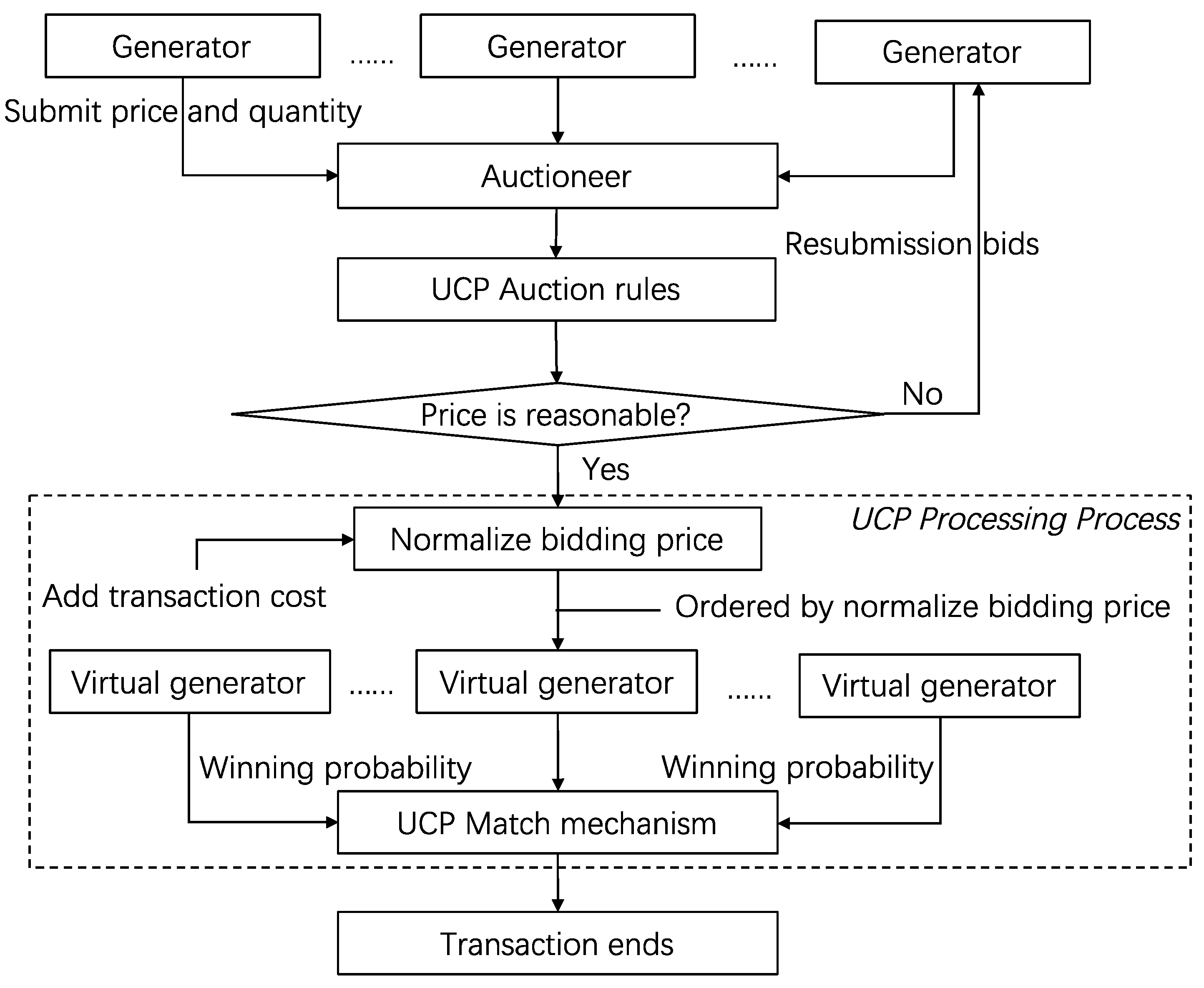
Figure 3.
Demand scenario effected on social welfare: (a) customer surplus comparison; (b) generator surplus comparison.
Figure 3.
Demand scenario effected on social welfare: (a) customer surplus comparison; (b) generator surplus comparison.


Table 1.
Transaction cost information [32].
Table 1.
Transaction cost information [32].
| 1 | 2 | 3 | 4 | |
| 0.120 | 0.220 | 0.303 | 0.372 |
Table 2.
Bidding results for a case study.
| Bidder | Private Cost | Bid Quantity | Optimal Bidding Price |
|---|---|---|---|
| 1 | 1.1425 | 1 | 1.2329 |
| 2 | 1.3510 | 3 | 1.4594 |
| 3 | 1.5499 | 1 | 1.6151 |
| 4 | 1.6221 | 2 | 1.6879 |
| 5 | 1.8530 | 1 | 1.8763 |
Table 3.
Bidding results with different demand scenario.
| Bidder | Private Cost | Bid Quantity | Optimal Bidding Price | |||
|---|---|---|---|---|---|---|
| 1 | 1.1425 | 1 | 1.2487 | 1.2529 | 1.2572 | 1.2617 |
| 2 | 1.3510 | 3 | 1.4534 | 1.4594 | 1.4667 | 1.478 |
| 3 | 1.5499 | 1 | 1.6093 | 1.6151 | 1.6224 | 1.6312 |
| 4 | 1.6221 | 2 | 1.6825 | 1.6879 | 1.6947 | 1.7033 |
| 5 | 1.8530 | 1 | 1.8734 | 1.8763 | 1.8801 | 1.8854 |
© 2018 by the authors. Licensee MDPI, Basel, Switzerland. This article is an open access article distributed under the terms and conditions of the Creative Commons Attribution (CC BY) license (http://creativecommons.org/licenses/by/4.0/).
Share and Cite
MDPI and ACS Style
Fang, D.; Ren, Q.; Yu, Q. How Elastic Demand Affects Bidding Strategy in Electricity Market: An Auction Approach. Energies 2019, 12, 9. https://doi.org/10.3390/en12010009
AMA Style
Fang D, Ren Q, Yu Q. How Elastic Demand Affects Bidding Strategy in Electricity Market: An Auction Approach. Energies. 2019; 12(1):9. https://doi.org/10.3390/en12010009
Chicago/Turabian StyleFang, Debin, Qiyu Ren, and Qian Yu. 2019. "How Elastic Demand Affects Bidding Strategy in Electricity Market: An Auction Approach" Energies 12, no. 1: 9. https://doi.org/10.3390/en12010009
Note that from the first issue of 2016, this journal uses article numbers instead of page numbers. See further details here.