Evaluating Magnetocaloric Effect in Magnetocaloric Materials: A Novel Approach Based on Indirect Measurements Using Artificial Neural Networks

Abstract

The thermodynamic characterisation of magnetocaloric materials is an essential task when evaluating the performance of a cooling process based on the magnetocaloric effect and its application in a magnetic refrigeration cycle. Several methods for the characterisation of magnetocaloric materials and their thermodynamic properties are available in the literature. These can be generally divided into theoretical and experimental methods. The experimental methods can be further divided into direct and indirect methods. In this paper, a new procedure based on an artificial neural network to predict the thermodynamic properties of magnetocaloric materials is reported. The results show that the procedure provides highly accurate predictions of both the isothermal entropy and the adiabatic temperature change for two different groups of magnetocaloric materials that were used to validate the procedure. In comparison with the commonly used techniques, such as the mean field theory or the interpolation of experimental data, this procedure provides highly accurate, time-effective predictions with the input of a small amount of experimental data. Furthermore, this procedure opens up the possibility to speed up the characterisation of new magnetocaloric materials by reducing the time required for experiments.

1. Introduction

Over the past two decades many research efforts have been focused on the development of not-in-kind refrigeration technologies [1], defined as alternative options to vapour-compression refrigeration systems. Among these, magnetic refrigeration shows promising results in terms of energy efficiency [1,2,3,4,5]. Furthermore, the scientific community is very interested because of the favourable environmental characteristics of this technology [6,7], which uses a solid substance as the refrigerant rather than the greenhouse-effect-promoting refrigerants used in vapour-compression applications. These latter refrigerants are being phased out [8,9], and they will need to be replaced. However, only a few pure fluids possess the combination of properties necessary for a refrigerant. Unfortunately, these fluids are at least slightly flammable [10]. In addition, some natural fluids, such as isobutane, propane or carbon dioxide, have been proposed as a solution. But, due to their flammability, hydrocarbons can only be employed in countries that permit their use [11]. On the other hand, the use of carbon dioxide is limited since it needs a high working pressure and this leads to poor performance in terms of energy [12,13].

The functioning of a magnetic refrigerator system is based on the magnetocaloric effect (MCE), the discovery of which is attributed to Weiss and Piccard [14]. The MCE is a feature of some magnetic materials that heat up when they are subjected to an external magnetic field, since the atoms, which act as magnetic dipoles, align with the magnetic field, and then cool down after the applied field is removed. They are called magnetocaloric materials (MCMs). The MCE is characterised by the directly measured temperature change of the MCM subjected to the external magnetic field. It can be evaluated as the isothermal entropy change $\Delta s_{iso}$ or the adiabatic temperature change $\Delta T_{ad}$ of the MCM induced by the increasing or the decreasing of an external magnetic field that the material is subjected to. If the conditions are kept adiabatic, the temperature of the MCM increases/decreases by the amount $\Delta T_{ad}$. On the other hand, if the conditions are kept isothermal, the specific entropy of the MCM decreases/increases by the amount $\Delta s_{iso}$.

One of the main problems associated with MCMs is related to the small MCE [15], which is not large enough to reach an appropriate temperature span for near-room-temperature applications, i.e., between 20 °C and 35 °C. A theoretical study about the maximum MCE achievable with an MCM, referring to a single-stage cooling device, was presented by Zverev et al. [16]. For achieving a larger temperature span, the prototypes built so far have been based on the active magnetic regenerative (AMR) cycle [17], which makes it possible to increase the temperature span between the heat sink and the heat source, so that it can be several times larger than the adiabatic temperature changes in an MCM. The AMR cycle is based on four operational steps (in the case of the Brayton thermodynamic cycle): an adiabatic magnetisation, isofield cooling, adiabatic demagnetisation and isofield heating. During the first step, the MCM is subjected to the external magnetic field and the temperature of the MCM increases due to the MCE. Then, keeping the magnetic field at a constant value, a fluid can flow through the material absorbing heat from it, which is subsequently rejected in the hot heat exchanger. In the adiabatic demagnetisation step, the external magnetic field is removed, and the MCM cools down. During the last step of the cooling cycle, with no external magnetic field, the fluid flows in a counter-flow direction through the material, expelling heat to it. Next, the fluid absorbs heat in the cold heat exchanger. The steps are then continuously repeated.

For room-temperature applications, starting from the construction of the first magnetic refrigerator prototype [18], several devices with different configurations and different magnetocaloric materials have been developed. In these prototypes, Gd and Gd-based alloys were the most commonly used MCMs [19,20,21,22,23,24,25]. Nevertheless, other substances have also been tested to evaluate their performances in magnetic refrigeration systems. These include La-Fe-Co-Si [26,27,28,29,30] and also Mn-Fe-P-As [31,32] alloys. Considering low-temperature applications, a comprehensive review about MCMs and devices for magnetic refrigeration in the temperature range of nitrogen and hydrogen liquefaction was performed by Zhang et al. [33]. Furthermore, a very recent review about magnetic refrigerator devices for room-temperature applications can be found in Gimaev et al. [34]. In addition to the experimental investigations, several AMR numerical models have been developed over the years, with the aim of studying different operating conditions and different MCMs in order to understand the feasibility of a magnetic refrigerator application [35,36].

The magnetocaloric properties required for AMR modelling, such as the adiabatic temperature change, can be obtained experimentally by employing direct and indirect methods [37,38,39]. The former is based on measurements of the temperature of the MCM sample subjected to an external magnetic field, thereby obtaining the adiabatic temperature change directly. The latter is based on heat-capacity and/or magnetisation measurements. With the indirect methods there are two routes to obtaining the magnetisation curves, depending on the temperature and the external magnetic field: the isofield process and the isothermal process. The isothermal measurement is the commonly used technique since it is faster. Hence, once the M (T, H) curves for the different temperatures and external magnetic fields are obtained, it is possible to calculate the isothermal entropy change and the adiabatic temperature change indirectly using Maxwell’s relations [37]. Another experimental method has been presented by Nielsen et al. [40], where the authors show an experimental device that can perform direct measurements of the magnetic entropy change.

Another approach to evaluating the adiabatic temperature change of MCMs is the application of theoretical models, which can be divided into two groups [41]: thermodynamic models and first-principle models. In particular, the formers are frequently used in the area of magnetic refrigeration to evaluate the magnetocaloric effect within numerical models of AMR cycles [42,43,44,45]. They identify a link among the magnetisation, the temperature and the external magnetic field using equations of state [41]. The most widely applied thermodynamic model for the calculation of the magnetocaloric effect is the Weiss mean field theory (MFT), which can be used to evaluate the total entropy of a ferromagnetic material as a function of the temperature and the external magnetic field [46] by considering the link with the magnetisation. The first-principle models are based on a calculation of the exchange-coupling energies and the magnetic moments of MCMs. They are usually performed to extract information about the values of magnetization at finite temperatures, the magnetic entropy, the magneto-structural transition temperatures, and the MCE, as shown in Paudyal et al. [47].

However, both the theoretical and experimental methods for evaluating the MCE have some important disadvantages. For example, the theoretical model (such as MFT) requires several material-based data that are not always known (in particular for new MCMs) and usually quite significantly over-predicts the MCE, as shown, for example, in Mugica Guerrero et al. [48]. On the other hand, the experimental methods are time-consuming and could be challenging to perform, especially in the case of direct measurements, where a high density of the data is required (as in the case of AMR modelling). Furthermore, it should be noted that there is no standardisation of the method for evaluating the magnetocaloric properties to characterise MCMs, which does not allow a direct comparison of the results. However, a correct and rapid evaluation of the magnetocaloric properties of an MCM, especially the adiabatic temperature change, and also isothermal entropy change and specific heat, is crucial to understanding the feasibility of using it in a magnetic refrigerator application.

In this study we propose a new MCMs-modelling method based on artificial neural networks (ANNs), which have been used in the past only for modelling the performance of AMR-based refrigerator devices [49,50]. This approach could represent a unique standardised method to evaluate the magnetocaloric effect and make it possible to reduce the experimental efforts to characterise known or new MCMs. A successful ANN can be used in the research field to produce results close to the experimental ones in a much faster way, providing sets of data which can be used for testing more detailed theories. Several mathematical models stemming from machine-learning algorithms were already applied with this purpose, such as the genetic algorithm [51], Bayesian approach [52] and ANNs themselves [53]. Furthermore, the ANN-based procedure can facilitate the implementation of the magnetocaloric properties of MCMs within an AMR numerical model. The latter represents the main advantage of this technique. Indeed, it is only necessary to perform the experiments at a few magnetic fields and temperatures to obtain a mathematical model of the magnetocaloric properties of the MCMs that can be easily included in an AMR numerical model. Then, the proposed ANN model can predict accurately the behaviour of the MCM for any magnetic fields and temperatures in between, ensuring a high density of the data needed for accurate AMR numerical simulations.

2. Materials and Methods

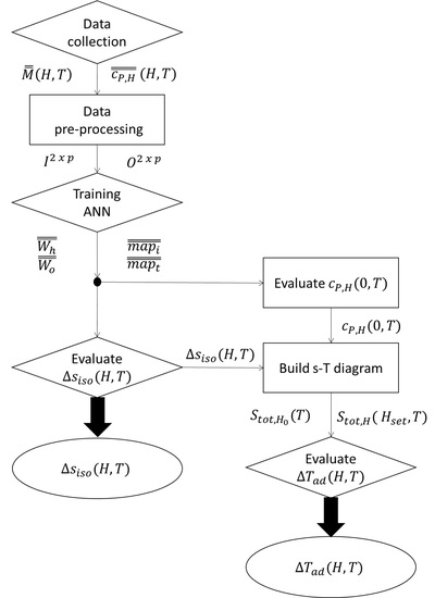
The ANN-based method is divided into four steps starting with the experimental phase that involves isothermal magnetisation and specific heat measurements at different magnetic fields and different absolute temperatures. Then, the collected data are processed to feed the development and the training of the ANN.

The ANN is a mathematical model inspired by the biological neural network in the human brain. An ANN is composed of several simple processing units, named neurons, which are connected to each other through weighted links, i.e., the synaptic weights. A neuron is characterised by three essential elements: a set of synaptic weights, a summation junction and an activation function. The first of these represents the strength of the relationships among adjacent neurons. The summation junction computes a weighted sum of the input and the activation function determines the output of the neuron itself. The main advantage of this model is related to its simplicity and ability to identify complex relationships between the input and the output using experimental data, without requiring any specific equation [50].

In order to define the ANN, it is necessary to specify the number of inputs, its architecture (i.e., the number of layers and the topology), the activation function of each layer and the training algorithm through which the knowledge-extraction process from the experimentations is run, modifying the free parameters of the network (synaptic weights). This task is accomplished by a training phase, during which the synaptic weights are modified to reduce the estimation error of the network. After the learning process, the ANN can predict the magnetisation and the specific heat of an MCM at each magnetic field and each absolute temperature within the range of the training dataset.

The third step foresees the calculation of the isothermal entropy change of the magnetocaloric material using the parameters of the ANN, which are the synaptic weights. In the last step, the adiabatic temperature change is evaluated by the construction of the s-T diagram, with the isothermal entropy-change values calculated in the previous step.

2.1. Experimental Setup and Data Collection

The first step of the ANN-based procedure is the experimental characterisation of the isothermal magnetisation and specific heat data. Two groups of materials were used to test the procedure: commercial gadolinium (Gd) and three different samples of LaFe_{13 − x − y}Co_xSi_y (hereto referred to as La-Fe-Co-Si) with exact compositions of (x = 0.86, y = 1.08), (x = 0.94, y = 1.01) and (x = 0.97, y = 1.07) and Curie temperatures of about 276 K, 287 K and 289 K, respectively. They are named Specimen 1, Specimen 2 and Specimen 3, respectively. For the purposes of this work the required experimental data were obtained from Bjørk et al. [26] The magnetisation measurements were performed with a vibrating-sample magnetometer (VSM), while the specific-heat data were collected with a differential scanning calorimeter (DSC) equipped with a magnetic field source. Furthermore, data relating to the adiabatic temperature change, measured with a type-E thermocouple (±0.1 K), were used to evaluate the performance of the entire ANN-based procedure. The experimental equipment and the procedures for the different tests are explained and presented in detail in Bjørk et al. [26] and Jeppesen et al. [54] It is important to note that all the measured values of the magnetocaloric properties were subsequently evaluated as a function of the internal magnetic field ${\mu }_0{H}_{int}$, which depends on the geometry of the sample (and the demagnetisation factor). Therefore, the thermodynamic properties were obtained as a function of ${\mu }_0{H}_{int}$. The latter is fundamental since the internal field ${\mu }_0{H}_{int}$ (subsequently referred to as H) is used as the input for the ANN in the second step. The output of this step is represented by the magnetisation and the specific heat experimental data of the MCMs, organised in matrix format (Equations (1) and (2)), where the values of the magnetic field H and the absolute temperature T are reported as rows and columns, respectively

$$\stackrel{\overline{¯}}{M}=\left[\begin{array}{ccccc}[]& T_1& T_2& \dots & T_v\\ H_1& M_{11}& M_{12}& \dots & M_{1v}\\ H_1& M_{21}& M_{22}& \ddots & ⋮\\ ⋮& ⋮& \ddots & \ddots & ⋮\\ H_u& M_{u1}& M_{u2}& \dots & M_{uv}\end{array}\right],$$

(1)

$$\stackrel{\overline{¯}}{c_{P,H}}=\left[\begin{array}{ccccc}[]& T_1& T_2& \dots & T_v\\ H_1& c_{P,H_{11}}& c_{P,H_{12}}& \dots & c_{P,H_{1v}}\\ H_1& c_{P,H_{21}}& c_{P,H_{22}}& \ddots & ⋮\\ ⋮& ⋮& \ddots & \ddots & ⋮\\ H_u& c_{P,H_{u1}}& c_{P,H_{u2}}& \dots & c_{P,H_{uv}}\end{array}\right].$$

(2)

2.2. Training the Artificial Neural Network

A multi-layer perceptron (MLP) with two inputs, one hidden layer and two outputs was used as part of the procedure to predict the behaviour of the MCMs (Figure 1).

The number of hidden layers can be greater than one, and it depends on the complexity of the problem. For very complex problems, such as vision and human language understanding, ANNs with more than one hidden layer (deep neural networks) can provide better performance [55], but considering approximation problems of continuous functions only one layer is sufficient to obtain good results [56]. If the approximation problem concerns non-continuous function, it may be necessary to use more than one hidden layer. In the framework of MCMs, this could happen considering first-order magnetic transition materials, characterised by a discontinuity in the magnetisation. The following equation describes the generalised mathematical model of an MLP with one hidden layer:

$$y_j={\phi }_o\left({{\displaystyle \sum }}_{k=1}^{N_h}{w}_{jk}\ast {\phi }_h\left({{\displaystyle \sum }}_{i=1}^{N_{il}}{w}_{ki}\ast x_i+b_k\right)+b_j\right),$$

(3)

where:

• $y_j$ is the output estimated j by the ANN;
• ${\phi }_o$ is the output-layer activation function;
• $N_h$ is the number of hidden neurons;
• $w_{jk}$ are the synaptic weights between the output j and the hidden neuron k;
• ${\phi }_h$ is the hidden-layer activation function;
• $N_{il}$ is the number of inputs;
• $w_{ki}$ are the synaptic weights between the hidden neuron k and the input i;
• $x_i$ is the input i to the ANN;
• $b_k$, $b_j$ are the bias of the hidden neuron k and the output j, respectively.

Considering the indirect method based on magnetisation measurements, the selected inputs for the model are represented by the magnetic field $H$, corrected for the demagnetisation factor, and the absolute temperature $T$. They are re-arranged in a matrix $I^{2 x p}$, where $p$ is the number of available experimental data, like the following:

$$I^{2xp}=\left[\begin{array}{cccc}{H}_1& H_2& \dots & H_p\\ T_1& T_2& \dots & T_p\end{array}\right].$$

(4)

As outputs, this architecture calculates the value of the magnetisation $M\left(H,T\right)$ and the specific heat at a constant magnetic field $c_{P,H}\left(H,T\right)$, corresponding to the magnetic fields and temperatures given. For each $p$, the ANN draws up the inputs according to the synaptic weights and provides the following output matrix:

$$O^{2xp}=\left[\begin{array}{cccc}{M}_1& M_2& \dots & M_p\\ c_{P,H_1}& c_{P,H_2}& \dots & c_{P,H_p}\end{array}\right].$$

(5)

The number of hidden neurons can be identified by employing a trial-and-error procedure [57,58] or using some empirical rules, as reported in [59]. There is no specific process to evaluate the optimal number of hidden neurons, but it must be identified case by case. In this study the evaluation of the number of hidden neurons was made by employing an iterative trial-and-error process. The minimum number of hidden neurons $N_{h,min}$ was identified using the following empirical rule [59,60]:

$$N_{h,min}=2\ast N_i+1,$$

(6)

where $N_i$ is the number of input neurons. Since the ANN has two inputs, the minimum number of hidden neurons was fixed at 5. Several ANNs were trained to vary the number of hidden neurons between the minimum and the selected maximum value. The latter was fixed at 15 units, but it can be changed to extend the range of the investigation. The activation functions selected for the hidden and output layers are the hyperbolic tangent (Equation (7)) and the linear one (Equation (8)), respectively:

$${\phi }_H\left(v_k\right)=\tanh \left(v_k\right)=\frac{2}{\left(1+e^{-2\ast v_k}\right)}-1,where{v}_k={{\displaystyle \sum }}_{i=1}^{N_i}{w}_{ki}\ast x_i+b_k,$$

(7)

$${\phi }_O\left(v_j\right)=v_j,\hspace{1em}\hspace{1em}\hspace{1em}\hspace{1em}where{v}_j={{\displaystyle \sum }}_{k=1}^{N_h}{w}_{jk}\ast H_k+b_j.$$

(8)

In Equations (7) and (8), the subscripts k and j refer to the k-th hidden neuron and the j-th output neuron. The term $v$ represents the induced local field of the neuron, which is the weighted sum of its inputs. The ANNs were trained using the standard error back-propagation (EBP) algorithm [61] with cross-validation [62], developed and performed with a code written in the MATLAB environment. The EBP algorithm can be divided into two steps: the forward pass and the backward pass. During the first one, the output of the ANN, fed with the input array $\left(x_1,x_2,\dots ,x_N\right)$, is calculated and then the error $e_j$ is evaluated in comparison to the target. This error is used to compute the correction $\Delta w_{jk}$ of the synaptic-weight values of the output layer. In the backward pass, the error is propagated towards the input layer, and the adjustment $\Delta w_{ki}$ of the synaptic-weight values of the hidden layer is calculated. The evaluation of the synaptic-weight changes is usually performed according to the steepest descent method [63] and can be expressed using the following equation:

$$\Delta w_{jk}=-\eta \ast \frac{\partial E\left(e_j\right)}{\partial w_{jk}},$$

(9)

where $\eta$ is the learning rate, and $E\left(e_j\right)$ is the error function. The error derivative of Equation (9) can be easily calculated through the derivative chain rule [61]. The learning rate for this application has been fixed at 0.3 after a trial-and-error procedure, but it can be modified according to needs. The batch-training method was used to perform the EBP. According to this learning technique, the synaptic weights are updated only when all the examples are fed into the ANN. The range between the processing of the first and the last experimental sample is named epoch. At the end of each epoch, the error metric is calculated, and the synaptic weights are updated according to Equation (9). This process is repeated until the stop condition is reached, which can be achieved when the error metric is lower than a target value or when the maximum number of epochs is reached. The Experimental data used as inputs and targets were normalised in the range of values between –1 and 1 (Equation (10)), as suggested in [64]:

$$x_n=-1+2\ast \frac{x-x_{min}}{x_{max}-x_{min}}.$$

(10)

This type of normalisation limits the value of the data within the domain of the hyperbolic tangent function. In Equation (10), $x$ represents either the input or output variables, $x_n$ is the corresponding normalised value, $x_{min}$ is the corresponding minimum value and $x_{max}$ is the corresponding maximum value. The cross-validation technique was used to avoid the overfitting of the experimental data, which can lead to poor generalisation capability. The initial dataset of the experimental data is divided into three different sub-sets: the training, validation and test sets. Only the first of these is used to modify the parameters of the ANN, i.e., the synaptic weights. The others are needed to evaluate the performance of the trained neural network when it observes data that are not included in the training dataset. Hence, the partition percentages must be defined to perform the cross-validation technique. In this procedure, the following values were fixed:

• 60% for the training set;
• 20% for the validation set;
• 20% for the test set.

Random extractions are performed from the entire dataset to build these different clusters. Furthermore, the order of the examples within the same subset is randomised at the beginning of each epoch. The training algorithm stops when the error function related to the validation set reaches the desired value. The most common error function used within the EBP algorithm is the mean square error (MSE), which is calculated as follows:

$$MSE=\frac{{{\displaystyle \sum }}_{j=1}^{N_o}{{\displaystyle \sum }}_{m=1}^p{\left(Y_{j,m}-y_{j,m}\right)}^2}{p\ast N_o}.$$

(11)

In Equation (11), $Y_{j,m}$ is the target value of the j-th output for the m-th example, $y_{j,m}$ is the output value predicted by the ANN of the j-th output for the m-th example, and $N_o$ is the number of output units. The latter assumes a value equal to 2 in this case. Furthermore, the mean absolute percentage error (MAPE), mean absolute error (MAE) and the determination coefficient (R²) are evaluated as performance indexes. These error metrics are calculated, respectively, as follows:

$$MAP{E}_j=\left|\frac{{{\displaystyle \sum }}_{m=1}^p\frac{\left(Y_{j,m}-y_{j,m}\right)}{Y_{j,m}}}{p}\right|\ast 100,$$

(12)

$$MA{E}_j=\left|\frac{{{\displaystyle \sum }}_{m=1}^p\left(Y_{j,m}-y_{j,m}\right)}{p}\right|,$$

(13)

$$R^2=1-\frac{{{\displaystyle \sum }}_{j=1}^{N_o}{{\displaystyle \sum }}_{m=1}^p{\left(Y_{j,m}-y_{j,m}\right)}^2}{{{\displaystyle \sum }}_{j=1}^{N_o}{{\displaystyle \sum }}_{m=1}^p{\left(Y_{j,m}\right)}^2}.$$

(14)

The second step of the procedure, starting from the experimental data of the isothermal magnetisation and the calorimetric measurements obtained for different magnetic fields and absolute temperatures, provides an ANN-based analytical formulation of the magnetisation and specific heat of the investigated sample. Hence, bearing in mind Equation (3), making appropriate substitutions also considering Equation (10), these properties can be expressed as follows:

$$M\left(H,T\right)=M_{min}+\frac{M_{max}-M_{min}}{2}\ast \left(1+{{\displaystyle \sum }}_{k=1}^{N_h}\left(w_{1k}\ast \tanh \left(v_h\left(H,T\right)\right)\right)+b_{j=1}\right),$$

(15)

$$c_{P,H}\left(H,T\right)=c_{P,H_{min}}+\frac{c_{P,H_{max}}-c_{P,H_{min}}}{2}\ast \left(1+{{\displaystyle \sum }}_{k=1}^{N_h}\left(w_{2k}\ast \tanh \left(v_h\left(H,T\right)\right)\right)+b_{j=2}\right),$$

(16)

where:

$$v_h\left(H,T\right)=w_{k1}\ast \frac{H_{min}+H_{max}-2H}{H_{min}-H_{max}}+w_{k2}\ast \frac{T_{min}+T_{max}-2T}{T_{min}-T_{max}}+b_k.$$

(17)

The Equations (15) and (16) make it possible to obtain the characteristic curves of the magnetisation and specific heat as functions of the magnetic field and absolute temperature, for each value within the training domain of the ANN. In detail, Equation (15) is proposed as an alternative mathematical formulation of magnetisation that can be evaluated by different magnetic phenomenological models, most of them based on the Weiss Mean Field Theory (MFT). The Equations (15) and (16) depend on the parameters of the ANN, which are the synaptic weights and the minimum and maximum values identified during the normalisation process. The synaptic weights are grouped within the matrixes of the synaptic weights $W_h{}^{N_{h}x(N_i+1)}$ and $W_o{}^{N_{o}x\left(N_h+1\right)}$, organised as follows:

$$\stackrel{\overline{¯}}{W_h}=\left[\begin{array}{ccc}{w}_{11}& w_{12}& b_1\\ w_{21}& w_{22}& b_2\\ ⋮& ⋮& ⋮\\ w_{k1}& w_{k2}& b_k\end{array}\right],$$

(18)

$$\stackrel{\overline{¯}}{W_o}=\left[\begin{array}{ccccc}{w}_{11}& w_{12}& \dots & w_{1k}& b_1\\ w_{21}& w_{22}& \dots & w_{2k}& b_2\end{array}\right],$$

(19)

where the subscript $k$ identifies the k-th hidden neurons. Considering $\stackrel{\overline{¯}}{W_h}$, the first and the second column are referred to as the first and the second input, i.e., the applied magnetic field and the absolute temperature, respectively. In $\stackrel{\overline{¯}}{W_o}$, the first and the second row are referred to the first and the second output, i.e., the magnetisation and the specific heat, respectively. The minimum and the maximum value of the input and output variables are grouped into two matrixes, named $ma{p}_i{}^{2x{N}_i}$ and $ma{p}_t{}^{2x{N}_o}$, respectively. They are organised as follows:

$$\stackrel{\overline{¯}}{ma{p}_i}=\left[\begin{array}{cc}{H}_{min}& T_{min}\\ H_{max}& T_{max}\end{array}\right],$$

(20)

$$\stackrel{\overline{¯}}{ma{p}_t}=\left[\begin{array}{cc}{M}_{min}& c_{P,H_{min}}\\ M_{max}& c_{P,H_{max}}\end{array}\right].$$

(21)

The matrixes from Equations (18) and (21) represent the result of the second and the input for the third step of the procedure introduced here. It is important to highlight that the training dataset does not include all the available experimental data. By exploiting the generalisation capability of the ANN, a reduced number of experimental tests was needed to carry out the predictions for the different materials. Specifically, a sensitivity analysis considering the different sizes of the training set was performed to point out the proper dimension of the dataset. Seven different training sets were developed, changing the number of magnetic field samples from 3 to 101 and considering only 11 temperature values. In Figure 2 the results of this analysis are reported.

Hence, 21 different values of the magnetic field, from 0 T to 1 T with a step of 0.05 T, and 11 different values of the absolute temperature, from 270 K to 310 K with a step of 5 K, plus 250 K and 260 K, were used to perform the learning phase.

2.3. Isothermal Entropy-Change Evaluation

Using Equation (15), the isothermal entropy change of the investigated MCM can be obtained by numerical integration for every desired step of both the magnetic field and the temperature. The latter can lead to an improvement of the modelling capability of the material properties, since it is possible to compute the evaluation with a small temperature step, reducing the systematic errors [65]. However, the properties defined for the ANN developed in the previous step can be used to evaluate the isothermal entropy change of the MCM via an indirect method using an analytical approach (Equation (22)). The EBP algorithm requires continuous and differentiable functions to be performed. Hence, the magnetisation formulation of Equation (15) makes it possible to calculate the magnetisation derivative concerning absolute temperature at a constant magnetic field, as follows:

$${\left(\frac{\partial M\left(H,T\right)}{\partial T}\right)}_H=\frac{M_{max}-M_{min}}{2}\ast {{\displaystyle \sum }}_{k=1}^{N_h}\left(\frac{2\ast w_{1k}\ast w_{k2}\ast sec{h}^2\left(v_h\left(H,T\right)\right)}{T_{max}-T_{min}}\right).$$

(22)

In Equation (22), $w_{1k}$ is the synaptic weight that links the first output, i.e., the magnetization of the specimen, to the k-th hidden neuron, whereas $w_{k2}$ is the synaptic weight that links the k-th hidden neuron to the second input of the ANN, which is the absolute temperature $T$. It is important to note that the synaptic weights used in this equation are linked to the derivative argument $M$ and the derivative variable T. The magnetization derivative value is used to calculate the isothermal entropy change using Maxwell’s relation. Hence, by analytical integration of Equation (22), the isothermal entropy change can be expressed as:

$$\begin{gathered} \Delta s_{iso}\left(H_1,H_2,T\right)={\mu }_0\frac{M_{max}-M_{min}}{2}\ast {{\displaystyle \sum }}_{k=1}^{N_h}\left(B\ast C\ast \left(\tanh \left(v_h\left(H_2,T\right)\right)- \\ \tanh \left(v_h\left(H_1,T\right)\right)\right)\right), \end{gathered}$$

(23)

where:

$$B=\frac{H_{max}-H_{min}}{T_{max}-T_{min}},$$

(24)

$$C=\frac{w_{1k}\ast w_{k2}}{w_{k1}}.$$

(25)

Equation (23) represents a new mathematical formulation of the isothermal entropy change based on ANN theory. The values of $H_2$ and $H_1$ are the final and the initial external magnetic fields of the process to which the specimen is subjected, respectively. In Equation (25), $w_{k1}$ is the synaptic weight that links the k-th hidden neuron to the first input of the ANN, which is the applied magnetic field H, i.e., the integration variable. Hence, using the output of the previous step, the isothermal entropy change can be straightforwardly obtained by Equation (23), avoiding the systematic errors caused by the numerical integration of Maxwell’s relation.

2.4. Adiabatic Temperature-Change Evaluation

The adiabatic temperature change $\Delta T_{ad}$ can be obtained from the isothermal entropy change, but the most accurate method used in numerical modelling is based on the construction of the s-T diagram of the MCM. The latter ensures an accurate and coherent evaluation of the magnetocaloric properties of the materials, which are correlated with the thermodynamic relations and are strongly dependent on the temperature and the magnetic field. The success of an AMR numerical model is strongly related to the correct prediction of these properties. The s-T diagram is built using the calculation of the total entropy $s_{tot}$ of the material. The evaluation of this property can be performed using different methods [37,40,66]. Another method is proposed in [67] where a protocol to perform the correct building of the s-T diagram for FOMT materials is described. In this procedure, the approach based on the use of the magnetisation data and the specific heat at zero magnetic field was implemented. The total entropy at zero field $s_{tot,H_0}\left(T\right)$ can be evaluated according to the following equation:

$$s_{tot,H_0}\left(T_1\right)=s_{ref}+{{\displaystyle \int }}_{T_{ref}}^{T_1}\frac{c_{P,H}\left(0,T\right)}{T}dT,$$

(26)

where $s_{ref}$ and $T_{ref}$ are the total entropy and the absolute temperature at the reference state, respectively, $T_1$ is the upper limit of the integration and $c_{P,H}\left(0,T\right)$ is the specific heat at zero magnetic field. For building the total entropy curves at different values of the magnetic field $s_{tot,H}$, it can proceed to add to isothermal entropy change calculated in the previous procedure step to the total entropy at zero magnetic field, as follows:

$$s_{tot,H}\left(H_{set},T\right)=s_{tot,H_0}\left(T\right)+\Delta s_{iso}\left(H_{set},T\right).$$

(27)

In Equation (27), $H_{set}$ is the applied magnetic field to which the MCM is subjected. In this way, the s-T diagram is completed, and the adiabatic temperature change $\Delta T_{ad}$ can be computed according to Equation (28), where $T_2\left(s_{tot,H_2}\right)$ is the temperature at the total entropy value along the curve of the magnetic field equal to $H_2$ and $T_1\left(s_{tot,H_1}\right)$ is the temperature at the total entropy value along the curve of the magnetic field equal to $H_1$:

$$\Delta T_{ad}=T_2\left(s_{tot,H_2}\right)-T_1\left(s_{tot,H_1}\right).$$

(28)

Hence, the last step of the procedure described in this paper considers the isothermal entropy change as the input and provides the adiabatic temperature change as the output. The implementation of the entire process was made by developing a code written in the MATLAB environment, which allows loading of the experimental data, developing and training the ANN, and calculating the isothermal entropy change and the adiabatic temperature change. The specific heat values are directly provided by the ANN trained with both the magnetisation and heat-capacity measurements, although they should be calculated from the total entropy curves (see Equation (29)) to ensure the thermodynamic consistency of the data within the AMR numerical model:

$$c_{P,H}\left(T\right)=T\ast {\left(\frac{\partial s_{tot,H}}{\partial T}\right)}_{H=const}.$$

(29)

However, the evaluation of the magnetocaloric properties of the MCMs performed here can be carried out using only the parameters of the ANN, i.e., the synaptic weights and the input-output mapping. Hence, once the ANN is trained, it needs only a small database to store information about these parameters for different MCMs. The code can be easily integrated into the existing and new numerical models, like that recently introduced in Mugica et al. [68].

3. Results and Discussion

3.1. Procedure Performance with Gadolinium

The ANN (refer to Appendix A for the ANN parameters) fits well both in terms of the magnetisation curves and the specific heat behaviour, as well as with data that the ANN was not trained for. The model predicts very well the trend of the specific heat near the Curie temperature: the peak value of specific heat decreases as the magnetic field increases and it shifts towards higher temperatures (see Figure 3b). Considering both outputs of the ANN (magnetisation and specific heat), an average mean absolute percentage error (MAPE) equal to 7.0% and an average determination coefficient (R²) of 0.9969 have been obtained.

By performing the third step of the procedure, the isothermal entropy change was calculated for the same conditions (magnetic fields and absolute temperatures) as in the previous step (see Figure 4). It is highlighted that in most cases the model predicts values of isothermal entropy change within the range of the error of the numerical solution [37].

The trend of isothermal entropy change as a function of temperature is also well predicted around the Curie temperature, where the isothermal entropy change shows its peak value.

From Figure 5b it is clear that the application of the ANN-based procedure leads to a slight underestimation of the adiabatic temperature change for all the magnetic fields, except for the maximum one. However, although these deviations are more pronounced for smaller magnetic fields, these differences are within the range of the error. Generally, it emerges that the trend of the adiabatic temperature changes as a function of temperature is preserved, also around the Curie temperature. It can be concluded that the model provides an estimation of the $\Delta T_{ad}$ with a mean absolute error (MAE) equal to 0.1 K and a maximum absolute error of 0.4 K. The determination coefficient between the measured and predicted values of the adiabatic temperature change is equal to 0.9871, which is close to the value obtained by Mugica Guerrero et al. [48].

In Figure 6 a comparison between the ANN-based procedure (introduced in this study), the direct-measurement method, and the MFT reported in Petersen et al. [45] is shown. It is evident that the MFT does not fit the experimental values of the specific heat particularly well. The values predicted by the ANN-based procedure are much closer to the measured ones, especially for H = 1 T. At zero field, some differences in the specific heat values occur around the Curie temperature. These deviations could be reduced by considering a smaller temperature step in the training set of the ANN around the Curie temperature. Furthermore, the MFT overestimates the adiabatic temperature change below the Curie temperature, with the most significant deviation from the experimental data at the Curie temperature. For temperatures above the Curie temperature, the deviations decrease. On the other hand, the prediction of the adiabatic temperature change using the developed ANN-based procedure is significantly better, within the error range of the experimental data (see Figure 6b), excluding just a few points at higher temperatures (between 306 K and 308 K).

3.2. Procedure Performance with the La-Fe-Co-Si Alloy

As shown in Figure 7, the predicted magnetisation and the specific heat values for the three specimens of La-Fe-Co-Si alloy fit well with the experimental results. For the Specimens 1–3, the MAPE values are equal to 8.5%, 6.6% and 6.5%, whereas the determination coefficients are 0.9980, 0.9946 and 0.9943, respectively.

The comparison of the isothermal entropy changes calculated with the ANN-based procedure and those obtained by the direct numerical integration of Maxwell’s relation shows a good agreement (see Figure 8). It is worth pointing out that, also in these cases, the ANN-based calculation process maintains the behaviour of the isothermal entropy change, highlighting a peak value around the Curie temperature for all the specimens. However, the predicted values for the isothermal entropy change of the three specimens are within the range of the error [37] in most cases.

The outcomes calculated in the fourth step of the procedure for the three samples of La-Fe-Co-Si alloy are shown in Figure 9, where in the left column (a–c) are the s-T diagrams, while in the right one (d–f), the adiabatic temperature changes are shown for four applied magnetic field values.

For all three samples, the MAE value related to the adiabatic temperature change was kept at 0.1 K, with a maximum between 0.2 K and 0.3 K. On the other hand, the R² values for Specimens 1–3 are equal to 0.9932, 0.9845 and 0.9907, respectively. The parameters of the ANNs developed for the La-Fe-Co-Si alloys are reported in Appendix B.

3.3. Summary of the Results

In

Table 1. Maximum values of the magnetocaloric properties of Gd and the three samples of La-Fe-Co-Si alloy at µ0H = 1 T from Bjørk et al. [26] and calculated by the ANN-based procedure.

	Gadolinium		Specimen 1		Specimen 2		Specimen 3
	Bjørk et al. [26]	This work	Bjørk et al. [26]	This work	Bjørk et al. [26]	This work	Bjørk et al. [26]	This work
ΔTad (1 T) [K]	3.3	3.3 (0.0%)	2.3	2.4 (+4.3%)	2.1	2.2 (+4.8%)	2.1	2.2 (+4.8%)
Tpeak [K]	295.1	294.9	277.1	276.3	287.1	286.7	289.6	288.1
|Δsiso (1 T)|[J/kgK]	3.1	3.0 (−3.2%)	6.2	5.9 (−4.8%)	5.1	5.2 (+2.0%)	5.0	5.3 (+6.0%)
Tpeak [K]	294.8	295.0	275.8	277.0	287.1	287.0	289.8	289.0
cp,H (1 T) [J/kgK]	298.8	295.0 (−1.3%)	783.4	776.6 (−0.9%)	754.9	748.8 (−0.8%)	740.9	743.7 (+0.4%)
Tpeak [K]	289.2	289.0	276.1	276.0	286.1	286.0	288.2	288.0

the maximum values of the adiabatic temperature change, the isothermal entropy change and the specific heat of the investigated MCMs are reported. These results show good agreement with the experimental data reported in Bjørk et al. [26], considering both the maximum values of the properties and the temperature at which these maxima occur (T_peak).

The performances shown by the ANN-based procedure with the different MCMs are summarised in

Table 2. Summary of the results carried out by implementing the ANN-based procedure with Gd and the three samples of La-Fe-Co-Si alloy.

		MAE		MAPE				ΔTad
MCM	Nh	M [A/m]	cp,H [J/kgK]	M [%]	cp,H [%]	Ave [%]	R2	R2	MAE [K]	Emax [K]
Gd	15	20681.1	2.6	13.0%	0.9%	7.0%	0.9969	0.9871	0.12	0.4
LaFe11.06Co0.86Si1.08	13	13504.0	7.4	15.8%	1.2%	8.5%	0.9980	0.9932	0.04	0.2
LaFe11.05Co0.94Si1.01	13	22975.9	3.5	12.7%	0.6%	6.6%	0.9946	0.9845	0.06	0.3
LaFe10.96Co0.97Si1.07	14	21518.0	5.3	12.1%	0.9%	6.5%	0.9943	0.9907	0.05	0.2

with respect to the error metrics (Section 2). In the second column the number of hidden neurons (N_h) is reported.

Considering the accuracy of the temperature sensor, the results reported in the previous sections and summarised in Table 2 prove the excellent prediction capability of the method. Hence, the application of the ANN-based procedure for two different materials led to similar error values (R² = 0.9871 for Gd against an average R² = 0.9895 for La-Fe-Co-Si alloy), demonstrating its capability to model the magnetocaloric properties of different types of MCMs.

The method introduced in this work provides thermodynamic properties for both evaluated groups of MCMs, making it possible to predict the magnetocaloric properties of both with reasonable accuracy. Furthermore, few data were used to train the ANN model, as described in Section 2. This fact represents a significant advantage, since the time needed to carry out the experiments decreases significantly. Indeed, computing the numerical integration with the same amount of data as used by the ANN-procedure could lead to up to 35% deviations of the maximum isothermal entropy change compared to the full data set measured with a step of 1 K [65].

Furthermore, the training parameters were kept unchanged. This makes it possible to perform the ANN procedure efficiently with different MCMs, by facilitating and speeding up the characterisation of new materials. To evaluate the magnetocaloric properties of an MCM by this procedure, one should measure the magnetisation and the specific heat at different temperatures and magnetic fields. Considering an arbitrary range, the temperature and the magnetic field steps which can be considered for the experiments are 5 K and 0.1 T, respectively. These values represent a guideline stem from the results reported in this work (see Figure 2). The volume of collected data depends on the chosen range. For example, if one wants to model the behaviour of an MCM in the magnetic field range between 0 T and 0.5 T (6 different values) and in the temperature range between 250 K and 350 K (21 different values), the volume of collected data will be equal to 126 for each output of the ANN, i.e., magnetisation and specific heat. Once the ANN is trained, the results could be verified and validated by analysing some intermediate points not considered during the ANN training. Hence, just a few other experiments are needed to validate the new ANN. However, some precautions have been taken when using the ANN-based procedure, related to the experimental part of the process. The results are strongly affected by the training phase of the ANN since the main thermodynamic properties are calculated using the synaptic weights identified during this step. The quality of the learning depends on the quality of the data with which the ANN is trained. Hence, it is necessary to make correct measurements of both the specific heat and the magnetisation. For the latter case, some indications can be found in the literature [41,65,69].

4. Conclusions

We propose a new and flexible procedure based on the use of ANNs to evaluate the thermodynamic properties of MCMs. It is shown that the procedure improves over the commonly used methods in the framework of magnetic refrigeration and provides similar or better results based on a reduced amount of information. Indeed, only a few experimental data are needed to perform a complete thermodynamic characterisation of an MCM, and no modifications to its general formulation are required. Hence, the tool developed in this work, available from the authors upon reasonable request, is proposed as a standardised procedure to evaluate the magnetocaloric properties of MCMs, which can improve the implementation of AMR numerical models and speed up the characterisation of new MCMs.

References

1. Qian, S.; Nasuta, D.; Rhoads, A.; Wang, Y.; Geng, Y.; Hwang, Y.; Radermacher, R.; Takeuchi, I. Not-in-kind cooling technologies: A quantitative comparison of refrigerants and system performance. Int. J. Refrig. 2016, 62, 177–192. [Google Scholar] [CrossRef] [Green Version]
2. Bansal, P.; Vineyard, E.; Abdelaziz, O. Status of not-in-kind refrigeration technologies for household space conditioning, water heating and food refrigeration. Int. J. Sustain. Built Environ. 2012, 1, 85–101. [Google Scholar] [CrossRef] [Green Version]
3. Kitanovski, A.; Plaznik, U.; Tomc, U.; Poredoš, A. Present and future caloric refrigeration and heat-pump technologies. Int. J. Refrig. 2015, 57, 288–298. [Google Scholar] [CrossRef] [Green Version]
4. US Department of Energy—Office of Energy Efficiency and Renewable Energy. Using Magnets to Keep Cool: Breakthrough Technology Boosts Energy Efficiency of Refrigerators. 2014. Available online: https://www.energy.gov/eere/articles/using-magnets (accessed on 23 July 2018).
5. US Department of Energy—Office of Energy Efficiency and Renewable Energy. ORNL Refrigerator Cools with Magnetism, Not Freon. 2016. Available online: https://www.energy.gov/eere/buildings/articles/orn (accessed on 23 July 2018).
6. EU Project 603885 Final Report Summary—ELICIT (Environmentally Low Impact Cooling Technology). 2017. Available online: https://cordis.europa.eu/result/rcn/201566_en.html (accessed on 25 July 2018).
7. EU Project 214864 Final Report Summary—SSEEC (Solid State Energy Efficient Cooling). 2013. Available online: https://cordis.europa.eu/result/rcn/57173_en.html (accessed on 25 July 2018).
8. UNEP. Twenty-Eighth Meeting of the Parties to the Montreal Protocol on Substances that Deplete the Ozone Layer. 2016. 1-9. Decision XXVIII/--- Further Amendment of the Montreal Protocol.
9. The European Commission. Regulation (EU) No 517/2014 of the European Parliament and of the Council of 16 April 2014 on Fluorinated Greenhouse Gases and Repealing Regulation (EC) No 842/2006. 2014. Available online: https://www.eea.europa.eu/policy-documents/regulation-eu-no-517-2014 (accessed on 26 July 2018).
10. McLinden, M.O.; Brown, J.S.; Brignoli, R.; Kazakov, A.F.; Domanski, P.A. Limited options for low-global-warming-potential refrigerants. Nat. Commun. 2017, 8, 1–9. [Google Scholar] [CrossRef] [PubMed]
11. Bansal, P.; Vineyard, E.; Abdelaziz, O. Advances in household appliances—A review. Appl. Therm. Eng. 2011, 31, 3748–3760. [Google Scholar] [CrossRef]
12. Aprea, C.; Greco, A.; Maiorino, A. The application of a desiccant wheel to increase the energetic performances of a transcritical cycle. Energy Convers. Manag. 2015, 89, 222–230. [Google Scholar] [CrossRef]
13. Llopis, R.; Cabello, R.; Sánchez, D.; Torrella, E. Energy improvements of CO2 transcritical refrigeration cycles using dedicated mechanical subcooling. Int. J. Refrig. 2015, 55, 129–141. [Google Scholar] [CrossRef]
14. Weiss, P.; Piccard, A. Le phénomène magnétocalorique. J. Phys. Théorique Appliquée 1917, 7, 103–109. [Google Scholar] [CrossRef]
15. Gschneidner, K.A.; Pecharsky, V.K. Rare earths and magnetic refrigeration. J. Rare Earths 2006, 24, 641–647. [Google Scholar] [CrossRef]
16. Zverev, V.I.; Tishin, A.M.; Kuz’Min, M.D. The maximum possible magnetocaloric ΔT effect. J. Appl. Phys. 2010, 107, 043907. [Google Scholar] [CrossRef]
17. Barclay, J.A. Use of a ferrofluid as the heat-exchange fluid in a magnetic refrigerator. J. Appl. Phys. 1982, 53, 2887–2894. [Google Scholar] [CrossRef]
18. Brown, G.V. Magnetic heat pumping near room temperature. J. Appl. Phys. 1976, 47, 3673–3680. [Google Scholar] [CrossRef]
19. Aprea, C.; Greco, A.; Maiorino, A.; Mastrullo, R.; Tura, A. Initial experimental results from a rotary permanent magnet magnetic refrigerator. Int. J. Refrig. 2014, 43, 111–122. [Google Scholar] [CrossRef]
20. Engelbrecht, K.; Eriksen, D.; Bahl, C.R.H.; Bjørk, R.; Geyti, J.; Lozano, J.A.; Nielsen, K.K.; Saxild, F.; Smith, A.; Pryds, N. Experimental results for a novel rotary active magnetic regenerator. Int. J. Refrig. 2012, 35, 1498–1505. [Google Scholar] [CrossRef]
21. Lozano, J.A.; Capovilla, M.S.; Trevizoli, P.V.; Engelbrecht, K.; Bahl, C.R.H.; Barbosa, J.R. Development of a novel rotary magnetic refrigerator. Int. J. Refrig. 2016, 68, 187–197. [Google Scholar] [CrossRef] [Green Version]
22. Romero Gómez, J.; Ferreiro Garcia, R.; Carbia Carril, J.; Romero Gómez, M. Experimental analysis of a reciprocating magnetic refrigeration prototype. Int. J. Refrig. 2013, 36, 1388–1398. [Google Scholar] [CrossRef]
23. Tagliafico, L.A.; Scarpa, F.; Valsuani, F.; Tagliafico, G. Preliminary experimental results from a linear reciprocating magnetic refrigerator prototype. Appl. Therm. Eng. 2013, 52, 492–497. [Google Scholar] [CrossRef]
24. Tušek, J.; Zupan, S.; Šarlah, A.; Prebil, I.; Poredoš, A. Development of a rotary magnetic refrigerator. Int. J. Refrig. 2010, 33, 294–300. [Google Scholar] [CrossRef]
25. Tura, A.; Rowe, A. Permanent magnet magnetic refrigerator design and experimental characterization. Int. J. Refrig. 2011, 34, 628–639. [Google Scholar] [CrossRef]
26. Bjørk, R.; Bahl, C.R.H.; Katter, M. Magnetocaloric properties of LaFe13-x-yCoxSi y and commercial grade Gd. J. Magn. Magn. Mater. 2010, 322, 3882–3888. [Google Scholar] [CrossRef]
27. Balli, M.; Sari, O.; Zamni, L.; Mahmed, C.; Forchelet, J. Implementation of La(Fe, Co)13-xSixmaterials in magnetic refrigerators: Practical aspects. Mater. Sci. Eng. B Solid-State Mater. Adv. Technol. 2012, 177, 629–634. [Google Scholar] [CrossRef]
28. Legait, U.; Guillou, F.; Kedous-Lebouc, A.; Hardy, V.; Almanza, M. An experimental comparison of four magnetocaloric regenerators using three different materials. Int. J. Refrig. 2014, 37, 147–155. [Google Scholar] [CrossRef]
29. Tušek, J.; Kitanovski, A.; Tomc, U.; Favero, C.; Poredoš, A. Experimental comparison of multi-layered La-Fe-Co-Si and single-layered Gd active magnetic regenerators for use in a room-temperature magnetic refrigerator. Int. J. Refrig. 2014, 37, 117–126. [Google Scholar] [CrossRef]
30. Pulko, B.; Tušek, J.; Moore, J.D.; Weise, B.; Skokov, K.; Mityashkin, O.; Kitanovski, A.; Favero, C.; Fajfar, P.; Gutfleisch, O.; et al. Epoxy-bonded La–Fe–Co–Si magnetocaloric plates. J. Magn. Magn. Mater. 2015, 375, 65–73. [Google Scholar] [CrossRef]
31. Kubacki, J.; Balin, M.K.; Kulpa, M.; Hawełek, Ł.; Włodarczyk, P.; Zackiewicz, P.; Kowalczyk, M.; Polak, M.; Szade, J. Magnetic moments and exchange splitting in Mn3s and Mn2p core levels of magnetocaloric Mn1.1Fe0.9P0.6As0.4and Mn1.1Fe0.9P0.5As0.4Si0.1compounds. Phys. B Condens. Matter 2017, 2, 2–7. [Google Scholar]
32. Szymczak, R.; Nedelko, N.; Lewińska, S.; Zubov, E.; Sivachenko, A.; Gribanov, I.; Radelytskyi, I.; Dyakonov, K.; Ślawska-Waniewska, A.; Valkov, V.; et al. Comparison of magnetocaloric properties of the Mn2-xFexP0.5As0.5(x = 1.0 and 0.7) compounds. Solid State Sci. 2014, 36, 29–34. [Google Scholar] [CrossRef]
33. Zhang, H.; Gimaev, R.; Kovalev, B.; Kamilov, K.; Zverev, V.; Tishin, A. Review on the materials and devices for magnetic refrigeration in the temperature range of nitrogen and hydrogen liquefaction. Phys. B Condens. Matter 2019, 558, 65–73. [Google Scholar] [CrossRef]
34. Gimaev, R.; Spichkin, Y.; Kovalev, B.; Kamilov, K.; Zverev, V.; Tishin, A. Review on magnetic refrigeration devices based on HTSC materials. Int. J. Refrig. 2019, 100, 1–12. [Google Scholar] [CrossRef]
35. Nielsen, K.K.; Tusek, J.; Engelbrecht, K.; Schopfer, S.; Kitanovski, A.; Bahl, C.R.H.; Smith, A.; Pryds, N.; Poredos, A. Review on numerical modeling of active magnetic regenerators for room temperature applications. Int. J. Refrig. 2011, 34, 603–616. [Google Scholar] [CrossRef] [Green Version]
36. Kamran, M.S.; Sun, J.; Tang, Y.B.; Chen, Y.G.; Wu, J.H.; Wang, H.S. Numerical investigation of room temperature magnetic refrigerator using microchannel regenerators. Appl. Therm. Eng. 2016, 102, 1126–1140. [Google Scholar] [CrossRef]
37. Pecharsky, V.K.; Gschneidner, K.A. Magnetocaloric effect from indirect measurements: Magnetization and heat capacity. J. Appl. Phys. 1999, 86, 565–575. [Google Scholar] [CrossRef]
38. Dan’kov, S.Y.; Tishin, A.; Pecharsky, V.; Gschneidner, K. Magnetic phase transitions and the magnetothermal properties of gadolinium. Phys. Rev. B Condens. Matter Mater. Phys. 1998, 57, 3478–3490. [Google Scholar] [CrossRef]
39. Lee, J.S. Evaluation of the magnetocaloric effect from magnetization and heat capacity data. Phys. Status Solidi Basic Res. 2004, 241, 1765–1768. [Google Scholar] [CrossRef]
40. Nielsen, K.K.; Bez, H.N.; Von Moos, L.; Bjørk, R.; Eriksen, D.; Bahl, C.R.H. Direct measurements of the magnetic entropy change. Rev. Sci. Instrum. 2015, 86, 103903. [Google Scholar] [CrossRef]
41. Franco, V.; Blázquez, J.S.; Ipus, J.J.; Law, J.Y.; Moreno-Ramírez, L.M.; Conde, A. Magnetocaloric effect: From materials research to refrigeration devices. Prog. Mater. Sci. 2018, 93, 112–232. [Google Scholar] [CrossRef]
42. Tušek, J.; Kitanovski, A.; Prebil, I.; Poredoš, A. Dynamic operation of an active magnetic regenerator (AMR): Numerical optimization of a packed-bed AMR. Int. J. Refrig. 2011, 34, 1507–1517. [Google Scholar] [CrossRef]
43. Liu, M.; Yu, B. Numerical investigations on internal temperature distribution and refrigeration performance of reciprocating active magnetic regenerator of room temperature magnetic refrigeration. Int. J. Refrig. 2011, 34, 617–627. [Google Scholar] [CrossRef]
44. Aprea, C.; Maiorino, A. A flexible numerical model to study an active magnetic refrigerator for near room temperature applications. Appl. Energy 2010, 87, 2690–2698. [Google Scholar] [CrossRef]
45. Petersen, T.F.; Pryds, N.; Smith, A.; Hattel, J.; Schmidt, H.; Høgaard Knudsen, H.J. Two-dimensional mathematical model of a reciprocating room-temperature Active Magnetic Regenerator. Int. J. Refrig. 2008, 31, 432–443. [Google Scholar] [CrossRef]
46. Brown, G.V. Magnetic Stirling Cycles—A new application for magnetic materials. IEEE Trans. Magn. 1977, 13, 1146–1148. [Google Scholar] [CrossRef]
47. Paudyal, D.; Pecharsky, V.K.; Gschneidner, K.A.; Harmon, B.N. Electron correlation effects on the magnetostructural transition and magnetocaloric effect in Gd5 Si2 Ge2. Phys. Rev. B Condens. Matter Mater. Phys. 2006, 73, 1–12. [Google Scholar] [CrossRef]
48. Mugica Guerrero, I.; Poncet, S.; Bouchard, J. Entropy generation in a parallel-plate active magnetic regenerator with insulator layers. J. Appl. Phys. 2017, 121, 074901. [Google Scholar] [CrossRef]
49. Chiba, Y.; Marif, Y.; Henini, N.; Tlemcani, A. Artificial Neural Networks Modeling of an Active Magnetic Refrigeration Cycle. In Artificial Intelligence in Renewable Energetic Systems. ICAIRES 2017; Lecture Notes in Networks and Systems; Hatti, M., Ed.; Springer: Cham, Switzerland, 2018; Volume 35. [Google Scholar]
50. Aprea, C.; Greco, A.; Maiorino, A. An application of the artificial neural network to optimise the energy performances of a magnetic refrigerator. Int. J. Refrig. 2017, 82, 238–251. [Google Scholar] [CrossRef]
51. Hartenstein, T.; Li, C.; Lefkidis, G.; Hübner, W. Local light-induced spin manipulation in two magnetic centre metallic chains. J. Phys. D Appl. Phys. 2008, 41, 164006. [Google Scholar] [CrossRef]
52. Neufcourt, L.; Cao, Y.; Nazarewicz, W.; Viens, F. Bayesian approach to model-based extrapolation of nuclear observables. Phys. Rev. C 2018, 98, 1–17. [Google Scholar] [CrossRef]
53. Pennington, R.S.; Coll, C.; Estradé, S.; Peiró, F.; Koch, C.T. Neural-network-based depth-resolved multiscale structural optimization using density functional theory and electron diffraction data. Phys. Rev. B 2018, 97, 1–10. [Google Scholar] [CrossRef]
54. Jeppesen, S.; Linderoth, S.; Pryds, N.; Kuhn, L.T.; Jensen, J.B. Indirect measurement of the magnetocaloric effect using a novel differential scanning calorimeter with magnetic field. Rev. Sci. Instrum. 2008, 79, 083901. [Google Scholar] [CrossRef] [Green Version]
55. Bianchini, M.; Scarselli, F. On the complexity of neural network classifiers: A comparison between shallow and deep architectures. IEEE Trans. Neural Netw. Learn. Syst. 2014, 25, 1553–1565. [Google Scholar] [CrossRef] [PubMed]
56. Cybenko, G. Correction: Approximation by superpositions of a sigmoidal function. Math. Control. Signals Syst. 1989, 2, 303–314. [Google Scholar] [CrossRef]
57. Sheela, K.G.; Deepa, S.N. Review on methods to fix number of hidden neurons in neural networks. Math. Probl. Eng. 2013, 2013, 425740. [Google Scholar] [CrossRef]
58. Mohanraj, M.; Jayaraj, S.; Muraleedharan, C. Applications of artificial neural networks for refrigeration, air-conditioning and heat pump systems—A review. Renew. Sustain. Energy Rev. 2012, 16, 1340–1358. [Google Scholar] [CrossRef]
59. Hunter, D.; Yu, H.; Pukish, M.S.; Kolbusz, J.; Wilamowski, B.M. Selection of Proper Neural Network Sizes and Architectures—A Comparative Study. IEEE Trans. Ind. Inform. 2012, 8, 228–240. [Google Scholar] [CrossRef]
60. Qian, G.; Yong, H. Forecasting the Rural Per Capita Living Consumption Based on Matlab BP Neural Shanghai University of Engineering Science. Int. J. Bus. Soc. Sci. 2013, 4, 131–137. [Google Scholar]
61. Rumelhart, D.E.; Hinton, G.E.; Williams, R.J. Learning representations by back-propagating errors. Nature 1986, 323, 533–536. [Google Scholar] [CrossRef]
62. Prechelt, L. Automatic early stopping using cross validation: Quantifying the criteria. Neural Netw. 1998, 11, 761–767. [Google Scholar] [CrossRef]
63. Jacobs, R.A. Increased rates of convergence through learning rate adaptation. Neural Netw. 1988, 1, 295–307. [Google Scholar] [CrossRef]
64. Jayalakshmi, T.; Santhakumaran, A. Statistical Normalization and Backpropagation for Classification. Int. J. Comput. Theory Eng. 2011, 3, 89–93. [Google Scholar] [CrossRef]
65. Neves Bez, H.; Yibole, H.; Pathak, A.; Mudryk, Y.; Pecharsky, V.K. Best practices in evaluation of the magnetocaloric effect from bulk magnetization measurements. J. Magn. Magn. Mater. 2018, 458, 301–309. [Google Scholar] [CrossRef]
66. Lozano, J.A.; Engelbrecht, K.; Bahl, C.R.H.; Nielsen, K.K.; Barbosa, J.R.; Prata, A.T.; Pryds, N. Experimental and numerical results of a high frequency rotating active magnetic refrigerator. Int. J. Refrig. 2014, 37, 92–98. [Google Scholar] [CrossRef] [Green Version]
67. Christiaanse, T.V.; Campbell, O.; Trevizoli, P.V.; Govindappa, P.; Niknia, I.; Teyber, R.; Rowe, A. A concise approach for building the s-T diagram for Mn-Fe-P-Si hysteretic magnetocaloric material. J. Phys. D Appl. Phys. 2017, 50, 365001. [Google Scholar] [CrossRef]
68. Mugica, I.; Poncet, S.; Bouchard, J. An open source DNS solver for the simulation of Active Magnetocaloric Regenerative cycles. Appl. Therm. Eng. 2018, 141, 600–616. [Google Scholar] [CrossRef]
69. Hansen, B.R.; Bahl, C.R.H.; Kuhn, L.T.; Smith, A.; Gschneidner, K.A.; Pecharsky, V.K. Consequences of the magnetocaloric effect on magnetometry measurements. J. Appl. Phys. 2010, 108, 043923. [Google Scholar] [CrossRef]
Figure 1. The adopted structure of the ANN. The magnetic field, in T, and the absolute temperature, in K, are the inputs of the ANN. The model provides the values of magnetisation, in A/m, and specific heat, in J/kgK, at the given magnetic field and absolute temperature. The subscript h refers to the synaptic weights between the hidden and the input layer. The subscript o refers to the synaptic weights between the output and the hidden layer. The index and the subscript k refer to the k-th neuron of the hidden layer.
Energies 12 01871 g001
Figure 2. Mean absolute error of the adiabatic temperature change predictions with different sizes of the training set at different magnetic fields. The number of temperature samples considered during the training of the ANNs has been fixed at 11.
Energies 12 01871 g002
Figure 3. Measured and predicted value at different magnetic fields: (a) Magnetization of Gadolinium, (b) Specific heat at a constant magnetic field of Gadolinium. The asterisk in the legend indicates an applied magnetic field not included in the training dataset.
Energies 12 01871 g003
Figure 4. Comparison between the isothermal entropy changes of gadolinium at different magnetic fields calculated with the ANN approach and those calculated by direct numerical integration. The asterisk in the legend indicates an applied magnetic field not included in the training dataset.
Energies 12 01871 g004
Figure 5. Results of the last step of the procedure: (a) s-T diagram of Gd and (b) adiabatic temperature change of gadolinium during the magnetisation phase at different magnetic fields. The asterisk in the legend indicates an applied magnetic field not included in the training dataset.
Energies 12 01871 g005
Figure 6. Comparison with MFT approach: (a) Measured values of specific heat of Gd at H = 1 T and H = 0 T in comparison with values predicted by the MFT approach and ANN-based procedure, (b) Measured values of the adiabatic temperature change of Gd at H = 1 T in comparison with the values predicted by the MFT approach and the ANN-based procedure.
Energies 12 01871 g006
Figure 7. Measured and predicted values at different magnetic fields: (ac) Magnetization of the three samples of La-Fe-Co-Si alloy, (df) Specific heat at a constant magnetic field of the three samples of La-Fe-Co-Si alloy. The asterisk in the legend indicates an applied magnetic field not included in the training dataset.
Energies 12 01871 g007
Figure 8. Comparison between the isothermal entropy changes of the three samples of La-Fe-Co-Si alloy at different magnetic fields calculated with the ANN approach and those calculated by numerical integration. The asterisk in the legend indicates an applied magnetic field not included in the training dataset.
Energies 12 01871 g008
Figure 9. Results of the last step of the procedure: (ac) s-T diagram of the three samples of La-Fe-Co-Si alloy and (df) adiabatic temperature change of the three samples of La-Fe-Co-Si alloy during the magnetisation phase at different magnetic fields. The asterisk in the legend indicates an applied magnetic field not included in the training dataset.
Energies 12 01871 g009