A Robust Feedback Path Tracking Control Algorithm for an Indoor Carrier Robot Considering Energy Optimization

1
School of Electrical Engineering, Shenyang University of Technology, Shenyang 110870, China
2
Center for Neuroscience and Biomedical Engineering, The University of Electro-Communications, Chofu, Tokyo 182-8585, Japan
3
School of System Engineering, Kochi University of Technology, Kochi 782-8502, Japan
*
Author to whom correspondence should be addressed.
Energies 2019, 12(10), 2010; https://doi.org/10.3390/en12102010
Submission received: 25 March 2019
/
Revised: 13 May 2019
/
Accepted: 22 May 2019
/
Published: 26 May 2019
(This article belongs to the Special Issue Robotics, Micronanosensor and Smart Devices for Control)
Abstract
:This work develops an indoor carrier robot for people with disabilities, where the precise tracking of designated route is crucial. The parameter uncertainties and disturbances of the robot impose significant challenges for tracking. The present paper first investigates the dynamic of mechanical structure and modeling of actuator motors and constructs a new dynamic model by considering all main parameter uncertainties and disturbances. A novel robust feedback tracking controller considering both the optimization of path tracking and the minimization of the power consumption energy is proposed. It is proved that the tracking errors e and satisfy a H∞ performance indicator while the energy consumption is minimum. A simulation example was performed and the results show that this novel algorithm can effectively reduce the tracking error from 0.2 m to 0.006 m while guaranteeing the minimum energy consumption. Furthermore, the effectiveness of the proposed method was validated by experiment compared with the non-robust one.
1. Introduction
In recent years, more and more countries have the lower fertility rates, which lead to ageing populations [1]. The shortage of labor is anticipated, and this will be a serious social problem soon. Consequently, to lead more convenient and safety lives, as well as to free young labor, robots are highly expected to support the daily life of humans at homes, offices, hospitals, and welfare facilities in the years to come [2]. Furthermore, with a rapidly increasing number of disabled people who need daily life help, life support robots to take caregivers’ roles are increasingly desirable to assist such people by endowing as much independence as possible [3]. Hence, many kinds of life support robots are being developed [4,5,6]. In the authors’ laboratory, a goods transport robot with automatic moving function based on a mobile platform has been developed [7].
To freely move in the narrow indoor environment, the mobile platform has the omnidirectional movement function by using three omnidirectional wheels. The mobile platform is a kind of typical three-wheel mobile robot, which consists of batteries, motors, motor drivers and controller. Note that the holonomic property enables robots to simultaneously self-rotate with the translational motion on a straight line. This capability works to an advantage over other types of robots in transport, tracking, and other missions in the uncertain and changing narrow indoor living environment. Since that the robot is working in a narrow indoor living environment, the precise tracking is vital. Moreover, the robot is powered by the batteries carried by itself; therefore, energy constraints are critical to the service time of the indoor carrier robots. Consequently, a high accuracy tracking control strategy considering energy optimization is necessary.
Several researchers have concentrated on the motion control of omnidirectional mobile robot owing to its highly coupled and random nonlinear dynamics, which is challenging for high-performance control system design [8,9,10]. As a critical performance, path and trajectory tracking has been studied extensively; for example, adaptive polar-space motion control [11], integral sliding mode control [12], hierarchical improved fuzzy dynamic sliding-mode control [13], motion control switching between two robust controllers [14], kinematic control combined with an integral sliding mode controller [15], robust adaptive tracking control [16], and model-predictive control with friction compensation [17], have been developed to improve tracking performance. Specifically, the authors of [11,15,16] investigated the adaptive, robust, and sliding mode control methods for the trajectory tracking and path following of omnidirectional mobile robot with parameter variations and uncertainties. However, they conducted studies using only the kinematic model. The authors of [12,13,14,17] developed the controller based on the robot’ dynamic model. However, they used the simplified dynamic model omitting the actuator motor dynamics. Few studies about path and trajectory tracking of omnidirectional robot have been done based on the dynamic model with consideration of the actuator motor dynamics. The indoor carrier robot for human support mainly works in a narrow, complex surrounding environment and needs contact with human beings. Therefore, the robot tracking systems are often affected by disturbances and the uncertainty of parameters in a vibration environment, which is more challenging. Moreover, most studies have not considered the energy optimization problem.
Robot systems are often powered by batteries; therefore, they are easily subjected to energy consumption efficiency problem, which significantly affect the operation time and feasibility in the works. Recently, with the development of robot technology, robot systems with high energy consumption have become important research topics [18,19,20,21,22,23,24,25,26,27,28,29,30]. An improved holistic approach, which adopts a hybrid heuristic accelerated by using multicore processors and the Gurobi simplex method for piecewise linear convex functions, is proposed to minimize energy consumption for the industrial robotics [18]. An energy consumption optimization scheme to determine the optimal base position and joint motion of a manipulator is proposed [19]. A novel multi-objective optimization method is developed for power optimization of a snake robot, which applies a particle swarm optimization combined with the pareto fronts method [20]. Several researchers focused on the energy optimization of biped walking robots, including the constrained quadratic programming and neuro-dynamic-based solver [21], a novel systematic architecture and algorithm of gait control for energy-efficiency optimization [22], and energy-optimal motion planning with kino-dynamic constraints [23]. Furthermore, energy optimization for mobile robots by path planning has drawn wide concern recently [24,25].
Note that few of the above studies consider the mobile robots’ energy optimization problem [26,27]. Furthermore, these rare studies on mobile robots’ energy optimization only consider the path planning method [28,29,30]. However, the problem of motion performance oriented to pathing tracking of a given path is neglected, which is crucial, as depicted above. In the case of power efficiency, designing a controller to achieve accurate tracking with fast and smooth response is not trivial. To our knowledge, no results considering both the energy efficiency and tracking accuracy for mobile robots have been reported. Consequently, determining how to maintain reliable tracking and ensure long-term autonomy works in the case of disturbances and the uncertainty of parameters in a vibration environment is a worthwhile endeavor.
Motivated by the above observations, the main contributions of this paper are as follows:
- (1)
- Since a dynamic model can more exactly formulate the driver-motion mechanism and the performance of actuator motor has a great influence on the performance of robot motion, in this paper, a new dynamic model considering simultaneously the mechanical and electrical systems for the indoor carrier robot is constructed. This new dynamic model is constructed by considering all parameter uncertainties and disturbances.
- (2)
- A path tracking controller combining an acceleration feedback controller with an improved robust compensation to successfully deal with the disturbances and the parameters changes is proposed. Especially, we introduce a time-varying decoupling-inverse matrix into the robust compensation based on the dynamic model, which is especially critical in the effectiveness of the compensation and robustness.
- (3)
- The proposed controller is proven to be globally asymptotically stable via the Lyapunov stability theory and the tracking error satisfies a specified robust specification, which is observed in a small neighborhood of zero. Considering the special application of the robot, the simulation results demonstrate the efficiency of the proposed scheme, while the new controller was validated by a path tracking experiment subjected to narrow, complex surrounding indoor environment.
The remainder of this paper is organized as follows. Section 2 describes the design of the structure and the kinetics analysis of the indoor carrier robot. Section 3 presents the design of the robust path tracking controller. The stability, tracking and energy consumption performance analysis are presented in Section 4. Section 5 and Section 6 show the simulations and experiment using the proposed method, respectively. Finally, we conclude this paper and state possible future research in Section 7.
2. Structure of the Indoor Carrier Robot and Its Modeling
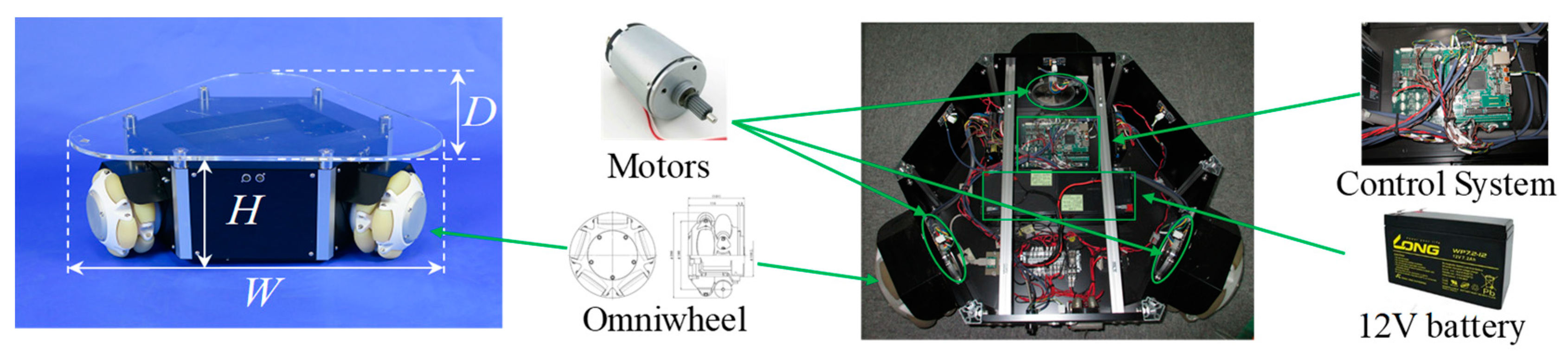
In this section, we introduce the structure of the indoor carrier robot and establish its dynamic models including actuators. An overview of our indoor carrier robot is shown in Figure 1. Three compact omni wheels are installed at the bottom corners of the robot to provide the robot with omnidirectional movement and thus achieve free movement in a narrow space. The three wheels are independently driven by three highly efficient, permanent, magnet-activated direct-current (DC) motors.
Figure 2 shows two usage examples of this robot. In Figure 2a, the robot helps the caregiver to carry the bookshelf to the bedridden person, while Figure 2b shows the robot carrying a package to the bedridden person. From the usage example of this robot, we notice that, when performing its task, the robot needs to go across the narrow places such as a door frame (as shown in Figure 2b). Therefore, in this condition, we must ensure the robot’s tracking accuracy to avoid colliding with the door frame. Moreover, the energy for indoor carrier robot is stored in the batteries that it carries, and this finite energy is consumed while performing the mission. Thus, to lengthen the use time of indoor carrier robot, strategies for reducing the energy of consumed by motors are desirable.
The values of the physical parameters of the indoor carrier robot are given in Table 1. The height of this movement platform is 0.275 m. Three omnidirectional wheels enable the support robot to move in any direction with the same orientation and free rotation. The maximum speed of the support robot is 1.96 m/s.
2.1. Modeling in Mechanical Systems
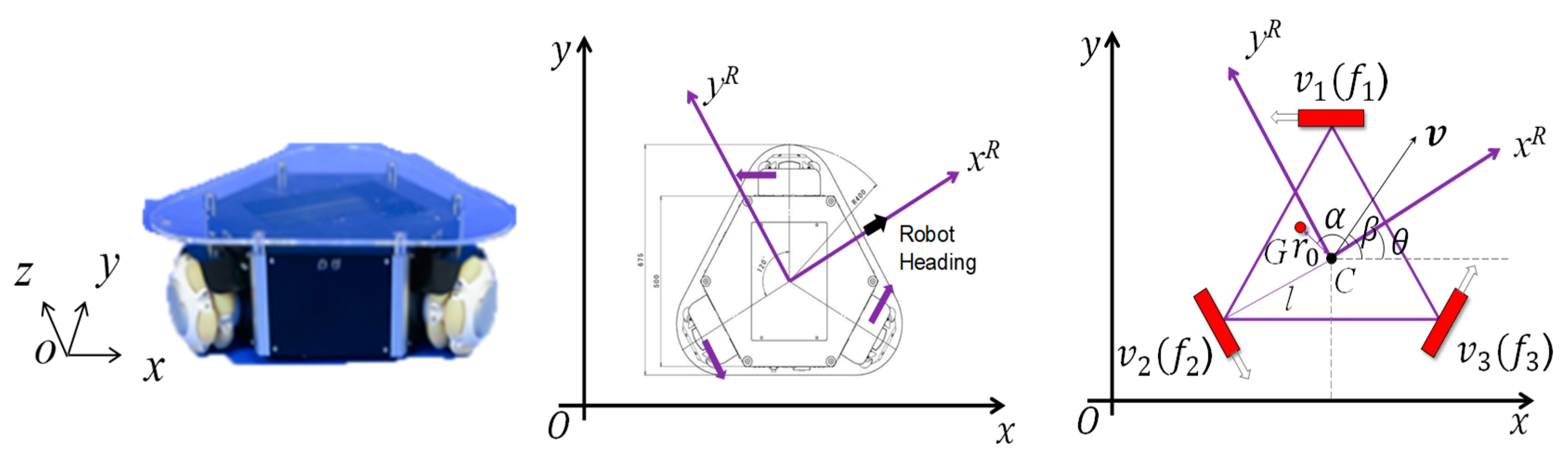
A schematic structure of the robot is shown in Figure 3. The kinematic and dynamic model analysis of the nonlinear system was carried by using the coordinate system shown in Figure 3.
In Figure 3, Σ(x, O, y) is the absolute coordinate system; Σ(xR, C, yR) is the robot coordinate system; θ is the orientation of the support robot; C denotes the position of the geometric center; G is the position of the center of gravity considering the effect of loads; r0 is the distance between the G and the C; α is the angle between xR axis and CG, which denote the offset angle of the center of gravity in the robot coordinate system; v is the speed of the indoor carrier robot; β is the moving direction of the robot; vi (i = 1, 2, 3) is the speed of each omni wheel; l denotes the distance from the center of the robot to each omni wheel; and f1, f2, and f3 are the driving forces of the three driving wheels.
Using the coordinate system shown in Figure 3, a kinematic analysis was carried out. The kinematic equation is shown in Equation (1) [7].
where
where and are the x and y components of the lift support robot’s velocity at center position, respectively.
According to the coordinate system shown in Figure 3, we analyzed the movement relationship between C position and G position, which is given as follows.
where
Considering the robot is carrying some goods, according to the rigid body dynamics, the motion of robot at center of gravity is given as follows [7]:
where
where M is the mass of the indoor carrier robot, m is the mass of goods, I is the inertial mass of the robot, and is the inertia mass caused by m. are the x and y components of the lift support robot’s acceleration at G, respectively; is angular acceleration of the robot around G; and ffriction1, ffriction2, and ffriction3 are the friction forces on the three wheels. The robot’s primitive load and center of gravity parameters are shown in Table 2.
According to Equation (2), we can get the robot’s acceleration relation between C and G position is
where is the time differentiation of the relation matrix .
Rearranging the dynamic in Equation (3) based on Equation (4), we can obtain the robot’s dynamics at position center position as the following [7].
Remark 1.
In practical applications, the difference of the load and the deformation of the mechanical structure, the coupling relationship between each force and robot’s motion (KG(θ)), center of gravity (r0, α) and mass of load (m) shown in Table 2 are changed. In addition, the friction is also nonlinear-time varying. These problems will lead to model perturbation in mechanical systems. The dynamic model in Equation (5) was constructed by considering the deformation of the mechanical structure, center-of-gravity shift, load changes and friction.
2.2. Modeling in Electrical Systems
It is assumed that the three DC motors have the same armature resistance Ra, back-emf constant ke, torque constant kt, and gear ratio n, as shown in Figure 4.
To simplify the dynamics, we ignore the inductance of the armature circuits because the electrical response is generally much faster than the mechanical response. The electrical circuit of the DC motor of each wheel is shown in Figure 4. Letting Vs be the battery voltage, the armature circuits of both motors are described by [31]:
where I = [i1 i2 i3]T denotes the armature current vector, U = [u1 u2 u3]T denotes the normalized control input vector, and ω = [ω1 ω2 ω3]T represents the angular velocity of each wheel. Superscripts 1, 2, and 3 correspond to the three motors in Figure 2, respectively.
In addition, the dynamic relationship between angular velocity and motor current, considering inertia and viscous friction [32], becomes
where Fv is the viscous friction coefficient and J = diag{J1, J2, J3} is the equivalent inertia matrix of the motors, which is symmetric. The values of the physical parameters of the drive motors are given in Table 3.
Remark 2.
In practical applications, the physical parameters of motors, Ra, ke, kt, and J will change with time and environment. This leads to the parameter perturbation problem, which will affect the control accuracy of the robot tracking system. Furthermore, the viscous friction Fv· ω will also affect the tracking accuracy. Therefore, we need to design proper controller to address these problems.
2.3. Robot Dynamics Combining the Mechanical and Electrical System
From Equations (6) and (7), the robot dynamic, considering the electrical circuit, can be written as:
Both sides of Equation (8) are divided by the radius of wheel r; since and , the driving force can be presenting by the control input vector and angular velocity.
Then, putting Equations (1) and (9) into the Equation (5), we can get the robot’s dynamic model considering electrical system as follows:
Remark 3.
The dynamic model of the previous study only considered the mechanical system, ignoring the effects of the electrical system. Therefore, in this paper, we take the electrical system into the consideration to improve the control accuracy, as shown in the model in Equation (10).
3. Tracking Control Strategy Design Considering Energy Optimization
The purpose of the present study was designing a feedback robust controller that could track the predefined paths to ensure that the robot can transport goods from an arbitrary initial position to the destination position when the robot is in an environment with uncertainty of center of gravity shift caused by goods and with random parameters. At the same time, the goal was to minimize the energy consumption.
Remark 4.
Indoor carrier robot is a class of typical wheeled robots that have omnidirectional movement function. To operate effectively in real-word applications, the control algorithm strategy must guarantee the robot can precisely follow a predesigned path. However, in practical applications, the various uncertainty factors including friction, load force, robot parameters perturbation, load change, center-of-gravity shift etc. seriously affect the tracking accuracy of the robot. Therefore, the design of the robust controller considering theses uncertain is important.
To analyze the robot system and design the control law, we first simplify the dynamics in Equation (10) as:
where
We assume that all these uncertainty factors can be treated as the additive model perturbation, therefore we decompose M1 and M2 based on the structure uncertainty characterize into the nominal part , and norm bounded perturbation part , . Therefore, the dynamic model in Equation (11) can be rewritten as:
Let the desired motion trajectory be XCd, and the actual motion trajectory be XC. Therefore, we define the tracking error as follows:
The purpose of the present section is to design a feedback robust controller such that the tracking error e and its time derivative tend toward zero as much as possible, while minimizing the energy consumption and maintaining all other signals in the closed-loop system to be probability bounded.
For the dynamic in Equation (10), a feedback robust controller with the compensation term is proposed.
where KD = diag(kDx, kDy, kDθ) and KP = diag(kPx, kPy, kPθ) are the design parameters. UH is the robust compensation term. Then, putting the control input in Equation (14) into the dynamic in Equation (11), the following equation is obtained.
Let all the parameter perturbation and model perturbation be the norm bounded perturbation
where γ > 0 denotes the upper bound of the parameter and model perturbation Then, Equation (15) can be rewritten as
Next, we design the robust compensation term UH to ensure the robot’s H∞ performance index. First, we let the state vector of the robot tracking system be as follows.
Then, we can get the following state equation.
That is,
Let,
Equation (19) can be rewritten as
Next, we design the H∞ compensation control input as
where R is a given positive definite symmetric matrix and P is the design control parameter, which is a positive definite symmetric matrix get by solving a Riccati equation as follows.
where γ > 0 is a given constant to determine the H∞ stiffness to the parameter uncertainty and external disturbance. Q is a positive set constant matrix, which satisfies the following inequality:
Figure 5 shows the robust feedback tracking control system.
4. Stability, Tracking, and Energy Consumption Performance Analysis
Theorem 1.
For the dynamic model of the indoor carrier robot with parameter uncertainty, model perturbation, and external uncertain disturbance considering the motor drive system (Equation (10)), the acceleration feedback controller (Equation (14)) under the action of robust compensation input (Equation (22)) and parameter matrix inequality (Equation (24)) are designed such that the tracking error model (Equation (21)) of the indoor carrier robot with bounded norm perturbation achieve asymptotic stability and the tracking error e andsatisfy the H∞ performance indicators (Equation (25)) and minimize the energy consumption performance indicators (Equation (26)).
wheredenotes the initial state of the robot. Q and R, the positive set constant matrix, are the weighted matrix, to decide the importance of the driving forces and tracking performance of each axis when achieving the optimal state. Q and R are the same as those in Equation (23).
The Proof of Theorem 1 is shown in Appendix A.
5. Simulations and Discussion
Four simulations were conducted to illustrate the feasibility, performance and merit of the proposed robust feedback tracking controller. The second simulation and fourth simulations were, respectively, performed to compare tracking performance with the non-robust controller.
5.1. Simulation Setting and Instructions
The aims of the simulations were to examine the effectiveness and performance of the proposed robust control law (Equation (22)) to the omnidirectional indoor carrier robot incorporated with effects of various uncertainties including friction, load force, robot parameters perturbation, load change, center-of-gravity shift, etc. Therefore, these simulations were conducted with the primitive robot parameters shown in Table 2 and Table 3 and the changed parameters affected by various uncertainties. To thoroughly simulate the complex route in a practical indoor environment, the robot was set to track two predefined paths.
All robot parameters included in the and of the control input (Equation (14)) were the primitive state shown in Table 1, Table 2 and Table 3. The selection of the feedback controller parameters is important for improving the motion accuracy of the robot. In this study, these parameters were selected referring to the method in [33] and simple manual adjustment based on the primitive state of the robot while tracking the rose path. To sufficiently evaluate the effectiveness of the proposed robust controller, the non-robust one and robust feedback controller were also evaluated using the same selected appropriate feedback controller parameters shown in Table 4.
The parameters of robust control law are as follows:
5.2. Simulation Results
5.2.1. Robust Rose Curve Trajectory and Path Tracking Result
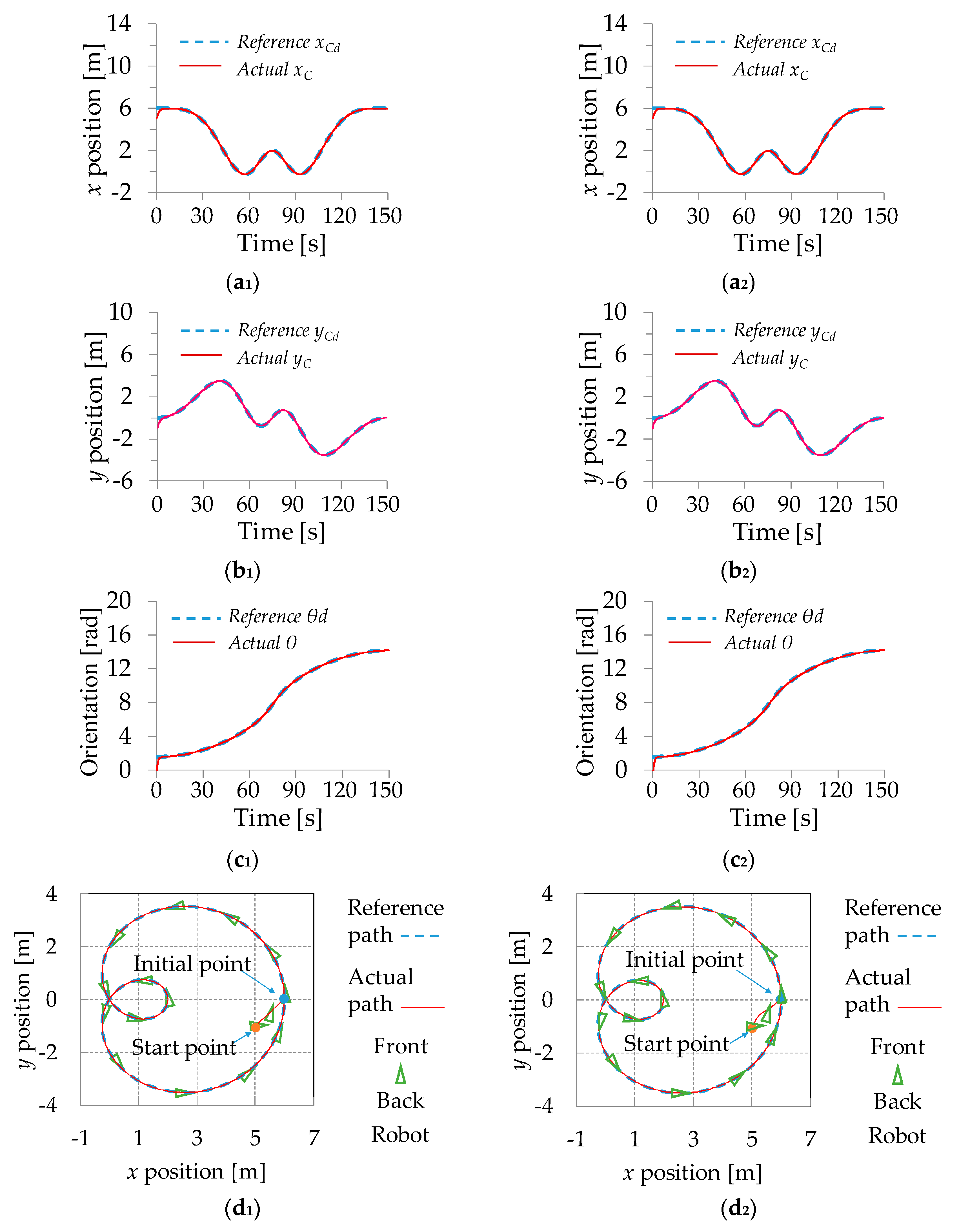
Two simulations were conducted to investigate the tracking performance of the robust control law (Equation (22)). The starting pose of the indoor carrier robot was assumed as [x(0) y(0) θ(0)]T = [5 m −1 m 0 rad]T while the whole time interval was [0 s 150 s]. In the first simulation, we set the robot to move along the special path and trajectory, called rose desired curve, which is expressed by
while the desired trajectory of each axis is expressed by
To make the proposed controller exhibit its robust performance to the parameters uncertainties, the simulation with parameters changes was carried out. Figure 6 depicts the tracking performance of proposed robust feedback controller to track the desired heart curve. Figure 6a1–d1 shows the results under the primitive parameters, while, Figure 6a2–d2 shows the tracking result after parameters of the robot changed. The tracking results in Figure 6a2–d2 are observed to be almost the same as the tracking results in Figure 6a1–d1. These results indicate that the proposed controller is capable of steering the omnidirectional indoor carrier robot to track the desired path and trajectories even with the described uncertainties.
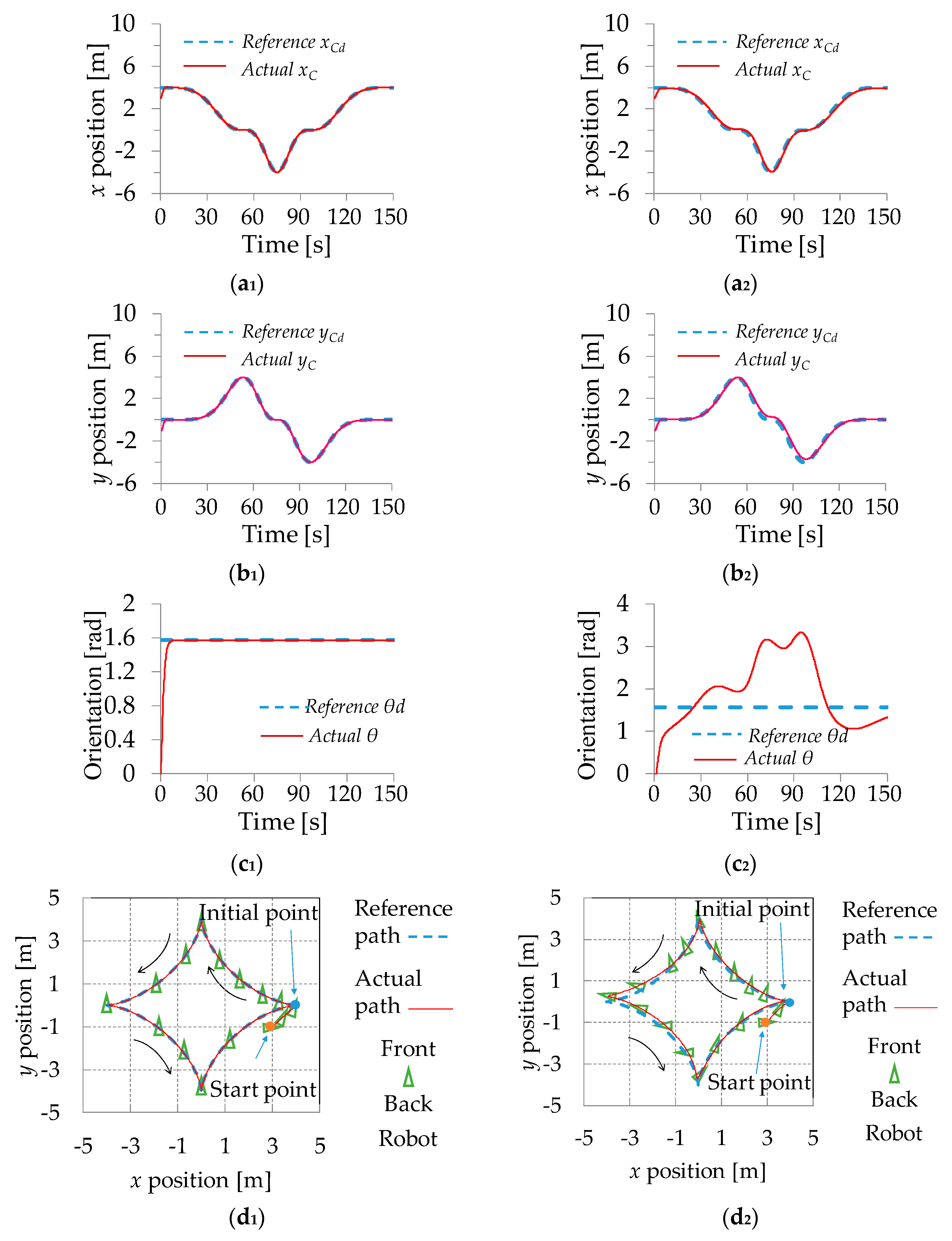
The second simulation was conducted to verify the superiority of the proposed robust control law (Equation (22)) with the non-robust feedback tracking control while we let the robust control law UH = 0. The tracking performance of non-robust feedback controller is shown in Figure 7. The tracking results under the changed parameters of robot are shown in Figure 7a2–d2 compared to the ones under primitive parameters shown in Figure 7a1–d1. These results show that non-robust controller can only roughly steer the robot to achieve trajectory and path tracking. Especially in Figure 7a2–d2, the robot almost cannot track the predefined path with robot parameters changes. These results indicate that the non-robust feedback tracking controller is not robust to the parameter changes, thus its tracking performance cannot be accepted in the narrow indoor environments. In comparison with Figure 7a2–d2, under the condition of parameter changes, the proposed robust controller has a smoother response to track the desired path shown in Figure 6a2–d2. These results also show that the proposed robust feedback tracking controller outperforms the non-robust one in tracking this special trajectory and path under parameters changes.
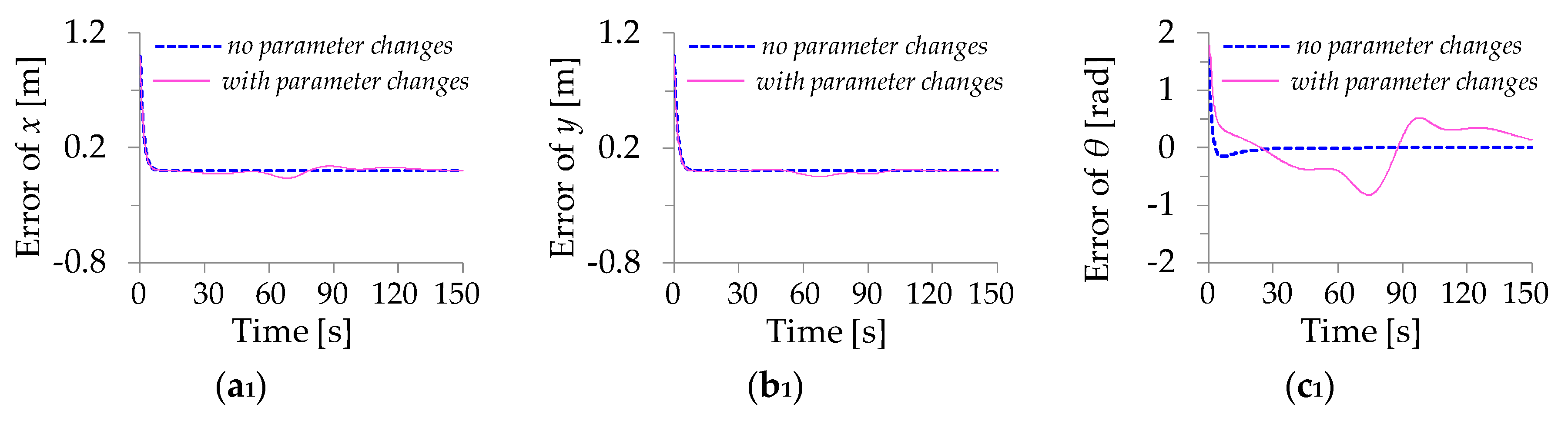
Furthermore, for the comparison, the convergent tracking errors of position and orientation of these two controllers are shown in Figure 8. Figure 8a2–c2 presents apparently larger tracking errors than those in Figure 8a1–d1. The results clearly reveal that the control law can steer the robot to track these special paths.
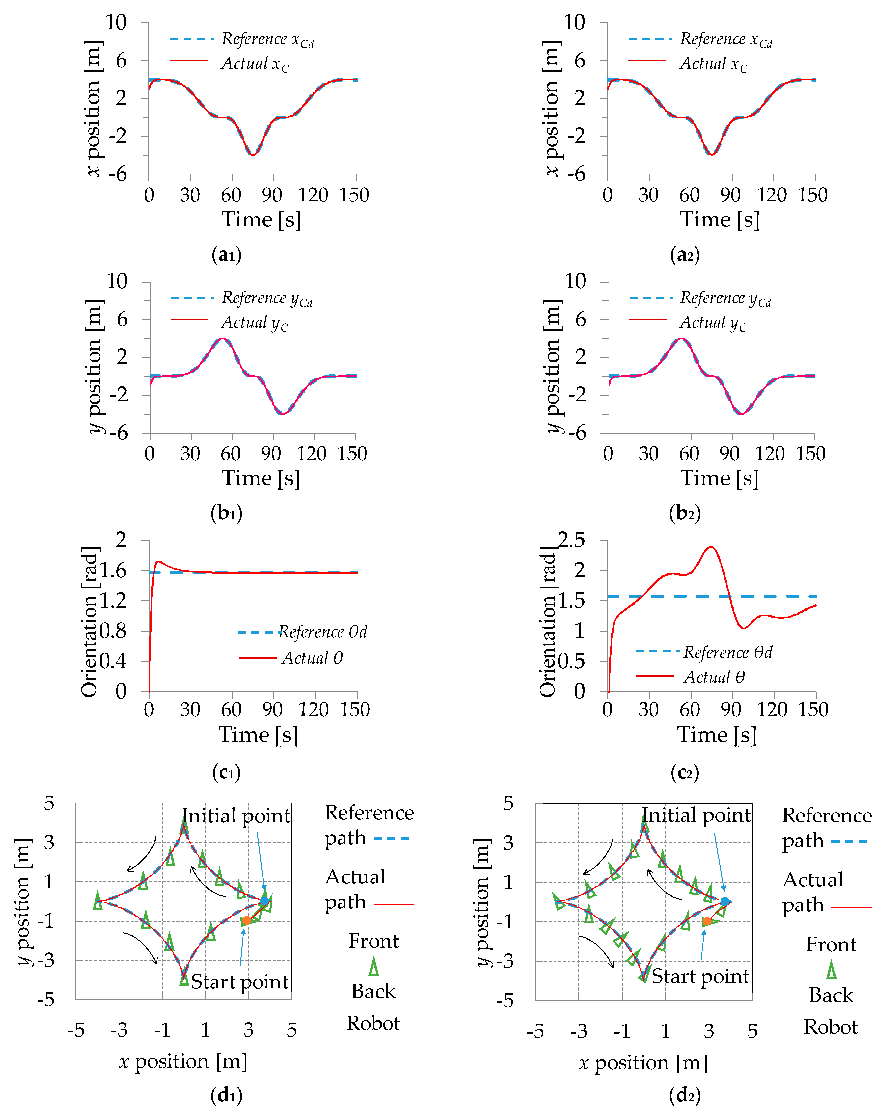
5.2.2. Robust Astroid Curve Trajectory and Path Tracking Result
This subsection investigates the tracking performance of the robust astroid curve path and trajectory tracking. The astroid curve path is expressed by:
and the desired trajectories of the position and orientation is defined as:
The starting pose of the indoor carrier robot was assumed as [x(0) y(0) θ(0)]T = [3 m −1 m 0 rad]T in the whole time interval [0 s 150 s]. Figure 8 shows the simulation results of the trajectory and path tracking using the proposed robust feedback controller. Figure 9a2–d2 presents the changed parameters tracking results, which indicate that the proposed controller can precisely steer the robot to achieve trajectory and path tracking for the astroid curve. The fourth simulation was conducted to compare the proposed robust controller with the non-robust one and the results are shown in Figure 10. Figure 9a1–d1 and Figure 10a1–d1 show that the two kinds controller have good tracking performance with the unchanged robot parameters. Figure 9a2–d2 and Figure 10a2–d2 depict the tracking performance of these two controllers for the changed robot parameters. Comparing these simulation results, the robust controller has better tracking performance for astroid path, even with the changed parameters.
Moreover, the trajectory tracking errors for the astroid of position and orientation of these two controllers were also considered; the detailed errors during tracking are depicted in Figure 11. These results visibly indicate the proposed H∞ compensation is capable of successfully steering the indoor carrier robot to track these special trajectories and show strong robust to the change of parameters changes.
5.3. Quantitative Analysis of Results and Discussion
The mean of trajectory tracking error for the two paths with parameter changes was calculated, and the result is shown in Table 5.
It can be seen in Table 5 that the tracking performance is significantly improved with the robust compensation.
The above simulation results demonstrated the effectiveness of the proposed robust method and verified that the indoor carrier robot with parameters uncertainty can provide accurate sequential motion.
6. Experiments and Discussion
The effectiveness of the proposed method was validated by experiments. The robot was set to track a circle path where the center and the radius were (0 m, 1 m) and 1 m, respectively. The desired trajectory is given as:
The initial position of the robot was (0 m, 0 m, 0 rad). To demonstrate the superiority of the robust controller, path tracking using a controller without robust compensation was also conducted. The two experimental path tracking results are shown in Figure 12, while the trajectory tracking errors of these two controllers are shown in Figure 13.
Figure 12 shows that satisfactory output tracking control was achieved. In particular, the tracking errors are significantly decreased using the designed robust compensation, as shown in Figure 13, which clearly indicates that the proposed controller enabled the robot to track the desired path despite parameter uncertainties and maintain good tracking results compared with the controller without the robust compensation. These results suggest that the controller can self-regulate its output values to adapt to changes in robot parameters. The control inputs are shown in Figure 14. Compared with the control inputs shown in Figure 14, the control inputs apparently changed to compensate for the varying friction. More specifically, we notice that the control inputs in Figure 14a are slightly larger than those in Figure 14b at the beginning. This is the self-regulating behavior adapting to the initial friction and uncertainty, which enables the initial errors of the proposed method to be smaller than those using the non-robust controller, as shown in Figure 13. u1 is rather larger around 2 s and 4.3 s, while u3 is significant around 3 s, u2 is slightly larger around 0.9 s in Figure 14a. These are some self-regulating behaviors adapting to the increased friction or robot parameter changes. Further, the control inputs in Figure 14a are less than those in Figure 14b during other time intervals, which show the energy-saving performance.
To specifically show the energy conservation of the proposed method, we quantitatively compared the two controllers based on these experiments. The energy consumption during experiments is calculated by . The robot consumed 105.69 kJ energy based on the robust controller while consumed 129.90 kJ energy when using the non-robust one. This result further shows the energy-saving performance of the proposed method.
To further show how well the proposed controller performs in a practice environment, a desired path that complies with a practice application in an actual family environment was designed to be tracked. The robot carried express goods from the vestibule to nearby the bed, as shown in Figure 15. It can be noticed that the robot needed go through a door frame whose width is 1.0 m, while the width of the robot is 0.733 m, as mentioned above. Hence, the path tracking error must be within 0.133 m, otherwise the robot would collide the door frame.
Four experiments were performed including path tracking experiments using proposed controller with and without goods, and the compared experiments using controller (non-robust compensation one) under the conditions of with and without goods. As with previous experiments, the control parameters of the two controllers were adjusted under the condition of without goods. The path tracking results are shown in Figure 15.
Figure 16a1 shows that the robot can smoothly track the desired path while the maximum path tracking error in door frame (narrowest space) is 0.03 m. This result indicates that the robot can smoothly go through the door frame based on the proposed controller. Furthermore, the maximum path tracking error is 0.08 m even if the robot has some load (Figure 16a2). This result suggests that the proposed controller can guarantee the robot’s smooth movement even with parameter changes in narrow spaces. On the contrary, Figure 16b1 shows the maximum path tracking error is 0.0117, which indicates that the robot has an almost permittable tracking performance using the non-robust compensation controller by properly adjusting the control parameters. However, when the robot has some load, the tracking error is 0.33 m (Figure 16b1). The robot would collide the door frame in this condition. The experimental results show that the robot can smoothly move in the corridor and go through the door frame based on proposed controller, even with parameter changes.
7. Conclusions
A new dynamic model for an indoor carrier robot considering the modeling of actuator motors is derived in this paper. To address the parameter uncertainties and disturbances problems, a new robust feedback acceleration controller is designed. Using the common Lyapunov function, we proved that the tracking results are consistent with a pre-programmed path designed such that the mean square of trajectory tracking errors e and satisfy a H∞ performance indicators while the energy consumption is at minimum. The obtained simulation results have demonstrated the effectiveness of the proposed method and verified that the indoor carrier robot with random parameters uncertainty can provide a precise motion while guaranteeing the minimum energy consumption. Additionally, the proposed controller was validated by experiments in an actual life environment. It is probable that, in addition the indoor carrier robot, the proposed method can also be applied to other wheeled mobile robots.
Author Contributions
Conceptualization, Y.W.; methodology, Y.W. and S.W.; software, W.X. and Y.J.; validation, Y.W. and J.Y.; formal analysis, Y.W.; investigation, Y.W.; resources, J.Y.; data curation, W.X.; writing—original draft preparation, Y.W.; writing—review and editing, J.Y. and Y.W. and funding acquisition, J.Y. and Y.W.
Funding
This research was funded by Ph.D. Start-up Fund of Natural Science Foundation of Liaoning Province, grant number 20170520449; the science and technology bureau project of Shenyang City, grant number 18013020; and the Liaoning Provincial Natural Science Foundation, grant number 20180550994.
Acknowledgments
The authors would like to thank the associate editor and the reviewers for their constructive comments and suggestions which help to improve the quality and clarity of the present paper.
Conflicts of Interest
The authors declare no conflict of interest.
Appendix A
Proof of Theorem 1.
Define the Lyapunov function:
Since P is a positive definite symmetric matrix, we get . The time derivative of V(t) based on the trajectory tracking error (Equation (13)), state variable (Equation (18)), and state equation (Equation (20)) becomes
Substituting the H∞ compensation control input (Equation (22)) and Riccati equation (Equation (23)) into Equation (28), we can get
Since the stability of the system is only related to the system structure and not related to the external input signal, we let the bounded norm perturbation be 0. Setting the Q and R as the positive constant matrix, it follows that,
On the other hand, by putting the H∞ compensation control input (Equation (24)) into the system state in Equation (23), we can the following system state equations.
Therefore, the system of the H∞ compensation control system is , according to the Riccati equation (Equation (23)), the following equation is established.
Since the new Riccati equation (Equation (A6)) has a positive solution, the system matrix is stable. Therefore, according to the Lyapunov stability (Equation (A1)), Equation (A3) and the solution of the Raccati equation, we can prove that the system in Equation (21) achieves the asymptotically stable.
Next, we analyze the H∞ tracking performance (Equation (25)) of the system. Define the control output of the system in Equation (21) as:
Define the tracking error performance index against to the bounded norm perturbation as:
Rearranging Equation (A8), we can get the following
Substituting Equation (A3) into Equation (A9), we can get
Then, according to the inequality in Equation (25), we can get the H∞ performance indicators
Furthermore, we analyze energy consumption performance indicators in Equation (26). First, according to the initial and final state of the robot, we introduce the follow formula:
Then, we put into Equation (A12), and, according to the state of Equations (A5) and (A3), we can get,
According to the Riccati equation (Equation (23)), Equation (A13) can be rearranged as:
Rearranging Equation (A14), we can get
The above formula shows that, when the control input is set as Equation (22), the performance index obtains the minimum values. □
References
- United Nations, Population Division: Department of Economic and Social Affairs. World Population Prospects: The 2017 Revision. Available online: https://www.un.org/development/desa/publications/world-population-prospects-the-2017-revision.html (accessed on 5 August 2018).
- Yamazaki, K.; Ueda, R.; Nozawa, S.; Kojima, M.; Okada, K.; Matsumoto, K.; Ishikawa, M.; Shimoyama, I.; Inaba, M. Home-Assistant Robot for an Aging Society. Brows. J. Mag. Proc. IEEE 2012, 100, 2429–2441. [Google Scholar] [CrossRef]
- Bien, Z.Z.; Chang, P.H.; Yoon, Y.S.; Park, K.H.; Park, S.H.; Park, S.; Do, J.; Lee, H.-E. Realization and evaluation of assistive human-mechatronic systems with human-friendly robotic agents at HWRS-ERC. In Proceedings of the IEEE 10th International Conference on Rehabilitation Robotics, Noordwijk, The Netherlands, 13–15 June 2007; pp. 328–334. [Google Scholar]
- Takei, T.; Imamura, R. Baggage carrier and navigation by a wheeled inverted pendulum mobile robot. IEEE Trans. Ind. Electron. 2009, 56, 3985–3994. [Google Scholar] [CrossRef]
- Cosma, C.; Confente, M.; Governo, M.; Fiorini, R. An autonomous robot for indoor light logistics. In Proceedings of the IEEE/RSJ International Conference on Intelligent Robots and Systems, Sendai, Japan, 28 September–2 October 2004; Volume 3, pp. 3003–3008. [Google Scholar]
- Hashimoto, K.; Saito, F.; Yamamoto, T.; Ikeda, K. A field study of the human support robot in the home environment. In Proceedings of the IEEE Workshop on Advanced Robotics and its Social Impacts (ARSO), Tokyo, Japan, 7–9 November 2013; pp. 143–150. [Google Scholar]
- Wang, Y.; Yang, J.; Wang, S. Path tracking control of an indoor carrier robot utilizing future information of the desired trajectory. Int. J. Innov. Comput. Inf. Control 2018, 14, 561–572. [Google Scholar]
- Borisov, A.V.; Kilin, A.A.; Mamaev, I.S. Dynamics and control of an omniwheel vehicle. Regul. Chaotic Dyn. 2015, 20, 153–172. [Google Scholar] [CrossRef]
- Raj, L.; Czmerk, A. Modelling and simulation of the drivetrain of an omnidirectional mobile robot. Automatika 2017, 58, 232–243. [Google Scholar] [CrossRef]
- Mamun, A.; Abdullah, M.; Nasir, M.T.; Ahmad, K. Embedded system for motion control of an omnidirectional mobile robot. IEEE Access 2018, 6, 1–18. [Google Scholar] [CrossRef]
- Huang, H.C.; Tsai, C.C.; Lin, S. Adaptive polar-space motion control for embedded omnidirectional mobile robots with parameter variations and uncertainties. J. Intell. Robot. Syst. 2011, 62, 81–102. [Google Scholar] [CrossRef]
- Hung, N.; Viet, T.D.; Im, J.S.; Kim, H.K.; Kim, S.B. Motion control of an omnidirectional mobile platform for trajectory tracking using an integral sliding mode controller. Int. J. Control Autom. Syst. 2010, 8, 1221–1231. [Google Scholar] [CrossRef]
- Hwang, C.L.; Yang, C.C.; Hung, J.Y. Path tracking of an autonomous ground vehicle with different payloads by hierarchical improved fuzzy dynamic sliding-mode control. IEEE Trans. Fuzzy Syst. 2018, 26, 899–914. [Google Scholar] [CrossRef]
- Alakshendra, V.; Chiddarwar, S.S. Simultaneous balancing and trajectory tracking control for an omnidirectional mobile robot with a cylinder using switching between two robust controllers. Int. J. Adv. Robot. Syst. 2017, 14. [Google Scholar] [CrossRef] [Green Version]
- Viet, T.D.; Doan, P.T.; Hung, N.; Kim, H.K.; Kim, S.B. Tracking control of a three-wheeled omnidirectional mobile manipulator system with disturbance and friction. J. Mech. Sci. Technol. 2012, 26, 2197–2211. [Google Scholar] [CrossRef]
- Huang, H.C.; Tsai, C.C. Adaptive robust control of an omnidirectional mobile platform for autonomous service robots in polar coordinates. J. Intell. Robot. Syst. 2008, 51, 439–460. [Google Scholar] [CrossRef]
- Lins, B.S.; Julio, C.; Scolari, C.; Andre, G.; Carlos, E.T.; Martinez, L.; de Pieriet, E.R. Design and implementation of model-predictive control with friction compensation on an omnidirectional mobile robot. IEEE ASME Trans. Mechatron. 2014, 19, 467–476. [Google Scholar]
- Bukata, L.; Sucha, P.; Hanzalek, Z. Energy Optimization of Robotic Cells. IEEE Trans. Ind. Inf. 2017, 13, 92–102. [Google Scholar] [CrossRef]
- Ma, C.; Gao, H.; Ding, L. Optimal energy consumption for mobile manipulators executing door-opening task. Math. Probl. Eng. 2018, 2018, 1–11. [Google Scholar] [CrossRef]
- Kelasidi, E.; Jesmani, M.; Pettersen, K.Y.; Gravdahl, J.T. Locomotion efficiency optimization of biologically inspired snake robots. Appl. Sci. Basel 2018, 8, 80. [Google Scholar] [CrossRef]
- Wang, L.; Chen, M.; Jiang, X.; Wang, W. Constrained quadratic programming and neuro-dynamics-based solver for energy optimization of biped walking robots. Math. Probl. Eng. 2017, 1–15. [Google Scholar] [CrossRef]
- Liu, Z.; Wang, L.; Chen, C.; Philip, L. Energy-efficiency-based gait control system architecture and algorithm for biped robots. IEEE Trans. Syst. Man Cybern. Part C-Appl. Rev. 2012, 42, 926–933. [Google Scholar]
- Zhou, X.; Jiang, L.; Guan, Y. Energy-optimal motion planning of a biped pole-climbing robot with kinodynamic constraints. Ind. Robot-Int. J. Robot. Res. Appl. 2018, 45, 343–353. [Google Scholar] [CrossRef]
- Wei, H.; Wang, B.; Wang, Y. Staying-alive path planning with energy optimization for mobile robots. Expert Syst. Appl. 2012, 39, 3559–3571. [Google Scholar] [CrossRef]
- Kim, H.; Kim, B.K. Online minimum-energy trajectory planning and control on a straight-line path for three-wheeled omnidirectional mobile robots. IEEE Trans. Ind. Electron. 2014, 61, 4771–4779. [Google Scholar] [CrossRef]
- Ganganath, N.; Cheng, C.T.; Fernando, T. Shortest path planning for energy-constrained mobile platforms navigating on uneven terrains. IEEE Trans. Ind. Inform. 2018, 14, 4264–4272. [Google Scholar] [CrossRef]
- Cao, F.; Liu, J. Optimal trajectory control for a two-link rigid-flexible manipulator with ODE-PDE model. Optim. Control Appl. Methods 2018, 39, 1515–1529. [Google Scholar] [CrossRef]
- Sun, Z.; Reif, J.H. On finding energy-minimizing paths on terrains. IEEE Trans. Robot. 2005, 21, 102–114. [Google Scholar] [Green Version]
- Liu, S.; Sun, D. Minimizing energy consumption of wheeled mobile robots via optimal motion planning. IEEE/ASME Trans. Mechatron. 2014, 19, 401–411. [Google Scholar] [CrossRef]
- Mei, Y.G.; Lu, Y.H.; Hu, Y.C.; Lee, C.S.G. Energy-efficient motion planning for mobile robots. In Proceedings of the IEEE International Conference on Robotics and Automation (ICRA), New Orleans, LA, USA, 26 April–1 May 2004; pp. 4344–4349. [Google Scholar]
- Rotich, W.C.; Rotich, S.T.; Nyamwala, F. Dynamic model of a DC motor-gear-alternator (MGA) system. Asian Res. J. Math. 2016, 4, 1–16. [Google Scholar]
- Maheriya, S.C.; Parikh, P.A. A review: Modelling of brushed DC motor and various type of control method. J. Res. 2016, 12, 18–23. [Google Scholar]
- Kilin, A.A.; Bozek, P.; Karavaev, Y.L.; Klekovkin, A.V.; Shestakov, V.A. Experimental investigations of a highly maneuverable mobile omniwheel robot. Int. J. Adv. Robot. Syst. 2017, 14, 1–9. [Google Scholar] [CrossRef]
Figure 1.
Appearance of the indoor carrier robot.

Figure 2.
Usage examples of the indoor carrier robot: (a) Carrying books; (b) Carrying a package.

Figure 3.
Structural model of the indoor carrier robot.

Figure 4.
The electrical circuit of the DC motor of each wheel.

Figure 5.
Block diagram of the path tracking control system.

Figure 6.
Trajectory and path tracking performance of the robust feedback tracking controller for the rose path (primitive parameters m = 6 kg, r0 = 0.2 m, α = π/2, Ra = 0.56 Ω, and Ffriction = 0: (a1) x position; (b1) y position; (c1) orientation θ; and (d1) path tracking) (changed parameters m = 26 kg, r0 = 0.3 m, α = π/3, Ra = 0.76 Ω, and Ffriction = [0.2 N, 0.2 N, 0.3 N∙m]: (a2) x position; (b2) y position; (c2) orientation θ; and (d2) path tracking).

Figure 7.
Trajectory and path tracking performance of the non-robust feedback tracking controller for the rose path (primitive parameters m = 6 kg, r0 = 0.2 m, α = π/2, Ra = 0.56 Ω, and Ffriction = 0: (a1) x position; (b1) y position; (c1) orientation θ; and (d1) path tracking) (changed parameters m = 26 kg, r0 = 0.3 m, α = π/3, Ra = 0.76 Ω, and Ffriction = [0.2 N, 0.2 N, 0,3 N∙m]: (a2) x position; (b2) y position; (c2) orientation θ; and (d2) path tracking).

Figure 8.
Trajectory tracking error for the rose curves (with robust compensation: (a1) x position; (b1) y position; and (c1) orientation θ) (non-robust compensation: (a2) x position; (b2) y position (c2); and orientation θ).
Figure 8.
Trajectory tracking error for the rose curves (with robust compensation: (a1) x position; (b1) y position; and (c1) orientation θ) (non-robust compensation: (a2) x position; (b2) y position (c2); and orientation θ).

Figure 9.
Trajectory and path tracking performance of the robust feedback tracking controller for the astroid path (primitive parameters m = 6 kg, r0 = 0.2 m, α = π/2, Ra = 0.56 Ω, and Ffriction = 0: (a1) x position; (b1) y position; (c1) orientation θ; and (d1) path tracking) (changed parameters m = 26 kg, r0 = 0.3 m, α = π/3, Ra = 0.76 Ω, and Ffriction = [0.2 N, 0.2 N, 0,3 N∙m]: (a2) x position; (b2) y position; (c2) orientation θ; and (d2) path tracking).

Figure 10.
Trajectory and path tracking performance of non-robust feedback tracking controller for the astroid path (primitive parameters m = 6 kg, r0 = 0.2 m, α = π/2, Ra = 0.56 Ω, and Ffriction = 0: (a1) x position; (b1) y position; (c1) orientation θ; and (d1) path tracking) (changed parameters m = 26 kg, r0 = 0.3 m, α = π/3, Ra = 0.76 Ω, and Ffriction = [0.2 N, 0.2 N, 0,3 N∙m]: (a2) x position; (b2) y position; (c2) orientation θ; and (d2) path tracking).

Figure 11.
Trajectory tracking error for the astroid curves (with robust compensation: (a1) x position; (b1) y position; and (c1) orientation θ) (non-robust compensation: (a2) x position; (b2) y position (c2); and orientation θ).
Figure 11.
Trajectory tracking error for the astroid curves (with robust compensation: (a1) x position; (b1) y position; and (c1) orientation θ) (non-robust compensation: (a2) x position; (b2) y position (c2); and orientation θ).


Figure 12.
Path tracking results of experiment with parameter changes: (a) with robust compensation and (b) non-robust compensation.
Figure 12.
Path tracking results of experiment with parameter changes: (a) with robust compensation and (b) non-robust compensation.

Figure 13.
Trajectory tracking errors (with robust compensation: (a1) x position; (b1) y position; and (c1) orientation θ) (non-robust compensation: (a2) x position; (b2) y position (c2); and orientation θ).
Figure 13.
Trajectory tracking errors (with robust compensation: (a1) x position; (b1) y position; and (c1) orientation θ) (non-robust compensation: (a2) x position; (b2) y position (c2); and orientation θ).

Figure 14.
Control inputs of the robot: (a) with robust compensation and (b) non-robust compensation.
Figure 14.
Control inputs of the robot: (a) with robust compensation and (b) non-robust compensation.

Figure 15.
One kind of working path in the actual family environment and its setting in two-dimensional coordinates.
Figure 15.
One kind of working path in the actual family environment and its setting in two-dimensional coordinates.

Figure 16.
Path tracking results (with robust compensation: (a1) no goods; and (a2) 10 kg goods on an off-center position) (non-robust compensation: (b1) no goods; and (b2) 15 kg goods on same position with (b1).
Figure 16.
Path tracking results (with robust compensation: (a1) no goods; and (a2) 10 kg goods on an off-center position) (non-robust compensation: (b1) no goods; and (b2) 15 kg goods on same position with (b1).


Table 1.
Physical Parameters of the wheeled mobile robot.
| Symbol | Quantity | Value and Unit |
|---|---|---|
| H | height | 0.275 m |
| W | width | 0.733 m |
| D | length | 0.635 m |
| M | mass | 40 kg |
| mmax | maximum load | 40 kg |
| I | inertia of mass | 0.68 kg·m2 |
Table 2.
Robot’s primitive load and center of gravity parameters.
| Parameter | Value | Parameter | Value |
|---|---|---|---|
| m | 0~40 kg | α | π/2 rad |
| r0 | 0.2 m | l | 0.423 m |
Table 3.
Parameters of the driver motors.
| Parameter | Value | Parameter | Value |
|---|---|---|---|
| Ra | 0.56 Ω | Fv | 0.054 Nm/(rad/s) |
| ke | 0.021 V/(rad/s) | Vs | 12 V |
| kt | 0.0280 Nm/A | r | 0.017 m |
| Ji(i = 1,2,3) | 0.0096 Nm/(rad/s2) | n | 1 |
Table 4.
Parameters of the feedback controller.
| Parameter | Value | Parameter | Value |
|---|---|---|---|
| kDx | 1.640 mg/s | kPx | 1.3066 mg/s2 |
| kDy | 1.640 mg/s | kPy | 1.3066 mg/s2 |
| kDθ | 2.11 Nm/A | kPθ | 4.11 kg·m2/s2 |
Table 5.
Mean of tracking errors (parameters changed).
| Robot Tracking | Errors of the Rose Curve | Errors of the Astroid Curve | ||
|---|---|---|---|---|
| Non-robust | With robust | Non-robust | With robust | |
| x position | 0.20 m | 0.0066 m | 0.13 m | 0.02 m |
| y position | 0.19 m | 0.0068 m | 0.16 m | 0.01 m |
| Orientation angle θ | 0.91 rad | 0.0314 rad | 0.69 rad | 0.34 rad |
© 2019 by the authors. Licensee MDPI, Basel, Switzerland. This article is an open access article distributed under the terms and conditions of the Creative Commons Attribution (CC BY) license (http://creativecommons.org/licenses/by/4.0/).
Share and Cite
MDPI and ACS Style
Wang, Y.; Xiong, W.; Yang, J.; Jiang, Y.; Wang, S. A Robust Feedback Path Tracking Control Algorithm for an Indoor Carrier Robot Considering Energy Optimization. Energies 2019, 12, 2010. https://doi.org/10.3390/en12102010
AMA Style
Wang Y, Xiong W, Yang J, Jiang Y, Wang S. A Robust Feedback Path Tracking Control Algorithm for an Indoor Carrier Robot Considering Energy Optimization. Energies. 2019; 12(10):2010. https://doi.org/10.3390/en12102010
Chicago/Turabian StyleWang, Yina, Wenqiu Xiong, Junyou Yang, Yinlai Jiang, and Shuoyu Wang. 2019. "A Robust Feedback Path Tracking Control Algorithm for an Indoor Carrier Robot Considering Energy Optimization" Energies 12, no. 10: 2010. https://doi.org/10.3390/en12102010
Note that from the first issue of 2016, this journal uses article numbers instead of page numbers. See further details here.