A Real Time Feed Forward Control of Slug Flow in Microchannels †


Department of Electrical, Electronics and Computer Engineering, University of Catania, v.le A. Doria 6, 95129 Catania, Italy
*
Author to whom correspondence should be addressed.
†
This paper is an extended version of the paper “Design of control systems for two-phase microfluidic processes” presented to the 24th Mediterranean Conference on Control and Automation (MED), Athens, Greece, 21–24 June 2016.
‡
These authors contributed equally to this work.
Energies 2019, 12(13), 2556; https://doi.org/10.3390/en12132556
Submission received: 28 March 2019
/
Revised: 17 June 2019
/
Accepted: 28 June 2019
/
Published: 3 July 2019
(This article belongs to the Special Issue Robotics, Micronanosensor and Smart Devices for Control)
Abstract
:In this work, the authors present a feed-forward control system for two-phase microfluidic processes, widely adaptable for system-on-chip control in a wide variety of bio-chemical experimental conditions, in which two fluids interact in a micro-channel. The proposed approach takes advantage of the optical monitoring of the slugs flow and the on-line signal processing in the frequency domain for slug passage detection. The experimental characterization of the slug flows by the frequencies of the slugs passage was obtained and used to drive the pumps. The open loop control system was designed and implemented in Labview. The platform includes four modules and a GUI. The first manages the communication between the PC and the syringe pumps, while the second is used to implement the control law. The third manages signal acquisition from the photo-diodes and the last implements the soft-sensor for the signal analysis. Wide-reaching experimental design was carried out for characterization and validation of this approach.
1. Introduction
Evaluation and assessment of microfluidics is a field of study that offers numerous benefits in various disciplines such as biology, chemistry and medical diagnostics. In particular, the two-phase processed modeling and control is one of the main challenges in the construction of complex microsystems, where fluids can circulate in a controlled manner performing a large number tasks in a maze of microchannels. A two-phase flow can be generated by two immiscible fluids (phase), or by one fluid and solid micro-particles mixed together. By the fluid-fluid interaction inside a micro-channel it can be reached different regimes [1] classified as: bubble, slug or plug, annular, churn and wispy annular. In this paper the slug flow regime was considered. In this context the combined effect of the curved geometry and the channel width in the range (–) [2] increases the process velocity (slug velocity) but, as well, the difficulty in the processes control. In this paper, the authors present a methodology for the real-time track and control of the slug flows in micro-channels that can be easily adapted in different contexts.
Based on the system theory definition, these microfluidic two-phase processes can be considered in the class of the two inputs and single output, nonlinear dynamical systems [3,4]. The control action on the microfluidic process can be obtained passively or actively. From one hand, a passive control to generate a desired flow can be implemented by exploiting the geometrical properties of the micro-channel, the physical properties of the fluids [5] and the micro-chip material [6]. On the other hand, thanks to the active control a desired flow can be reached in a precise and rapid manner but at higher cost due to interaction between the fluids and the external forces [7,8,9].
In this paper, the authors present an extended study for the definition of a control methodology, previously introduced in [10], that can be easily adapted in different contexts. This solution is based on a data-drive active control and an optical approach to detect in real time the slug’s frequency passage. In recent studies carried out by the authors, optical signals were used to characterize the flow nonlinearity [3,4] and some parameters have been introduced to classify and identify the slug flow inside the micro-channel [11,12,13]. Furthermore, this work proves the feasibility of using this information to tune the actuation system in real time.
In Section 1 the experimental design set-up is described in details: the microfluidic channel geometries, the input flow rates used, the fluids, and the equipment. In particular the fluids used are air and water deionized. The air can show very large change of density when a stress is applied, so in general conditions it is considered a compressible fluid. When we are referring to gas-liquid flow in a micro-channel different regimes can be detected based on the input flow rates, the characteristic of the two fluids and the diameter of the microchannel [1,14]. Even if a regime is reached, to track the flow inside the microchannel is really complex. In the case of slug flow the changes of the volume of the air under pressure conditions it is greater than the changes of a fluid. This aspect increases the level of the slug passage unpredictability and the flow irregularity. The data-driven control aims to overcome this issue; indeed the real-time control is based on the continuous optical monitoring of the process using low cost equipment avoiding any needs of a-priori knowledge or expectancy on the flow behavior.
In Section 2, control law definition, the signal analysis method for the flow dynamic characterization is presented and used to design a control system in order to impose the desired dynamics to the system. Section 3 then describes the implementation of the feed-forward control strategy implemented in Labview and the real-time experimental results obtained.
2. Experimental Design
In the experimental design a continuous bubble flow was generated by pumping deionized water and air at the Y-junction of a snake microchannel made in COC (Cyclic Olefin Copolymer), in the serpentine micro-channel (, , , Thinxxs).
Two syringe pumps (Cetoni, Nemesys) were connected to the microfluidic channel inlets by means of latex tubes. Generally, the pressure driven pumps lead greater level of flow stability, precision and response time but in this context the process unpredictability is an advantage to test the robustness of the control methodology investigated. Those advantages will be highlighted when it will be implemented the closed loop control. The micrometric size of the microfluidic system requires an optical instrumentation for image magnification, so a specifically designed electro optical system with X20 magnification objective was used (details in [12]).
The optical system allows for a parallel acquisition of light intensity variations by means of a photodiode-based circuit (SLD , Silonex), and a CCD (, Thorlabs) with frame rate of . A data acquisition module (, National Instrument) converts the voltage signals acquired from the pair of photodiodes with a sample rate of . The CCD active area is while the photodiode active area is equal to . The optical information was acquired and the process was monitored at the centre of straight part (labeled B). The signals acquired from the photo-diodes were also filtered. The flow diagram of the experimental set-up is shown in Figure 1.
The two input flow rates (V) were set equal (V = = ). A total of 18 experiments were repeated three times and then analysed. Each experiment lasted . Two ranges of input-flow rate were investigated:
- with a step of ;
- with a step .
All the experiments are summarized in Table 1.
Also the Capillary number for each experiment was computed, Table 2. It is in the range of , which confirms the theoretical expectancy of the droplet/slug formation [1].
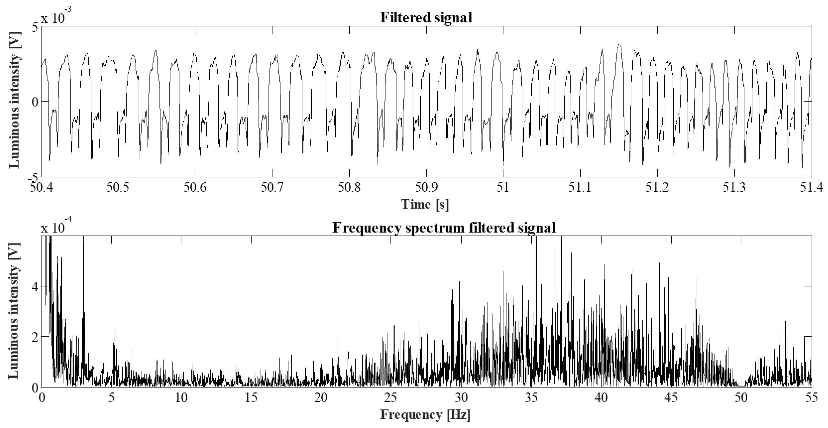
At the top, Figure 2 and Figure 3 highlight a zoom of the filtered signals in time domain, respectively, for and , the purpose is to show the trend of the acquired optical signals in the slowest and fastest experimental conditions considered (input flow rates). It is possible to distinguish clearly the air and water passages in the optical signal. The top level reveals the water presence, the middle value the air passage, and two lowest peaks are for the air slug front and rear. The luminosity level is slower in the air slug contour than the water slug contour being the water refraction index closer to the COC one.
Furthermore, these figures show as the increase in the flow rate affects the trend of the signal.
2.1. Slug Flow Detection
The control of the slug flow was obtained thanks to the development of an on-line signal processing approach for slug flow detection. Starting from the optical signal monitoring, an automatic procedure for the flow characterization in frequency domain was implemented. The focus of this work is not to develop a control system for a specific experimental condition but to study an approach that can be easily extended in other contexts. Generally, the liquid-liquid bi-phase dynamics are more stable than the liquid-gas one, so the control strategy investigated is expected to be easily applied. Additionally, thanks to the optical monitoring set-up used, tracking the slug passage at higher frequencies of droplet formation would be possible by increasing the acquisition frequency of the Data Acquisition Board.
At the bottom, Figure 2 and Figure 3 highlight a zoom of the filtered signals in frequency domain, respectively, for and , the purpose is to evidence how the increase in the flow rate affect the signal spectrum. Specifically, the signal in Figure 2 and Figure 3 show that the peak in the spectra is positioned at higher frequencies in experiment compared to .
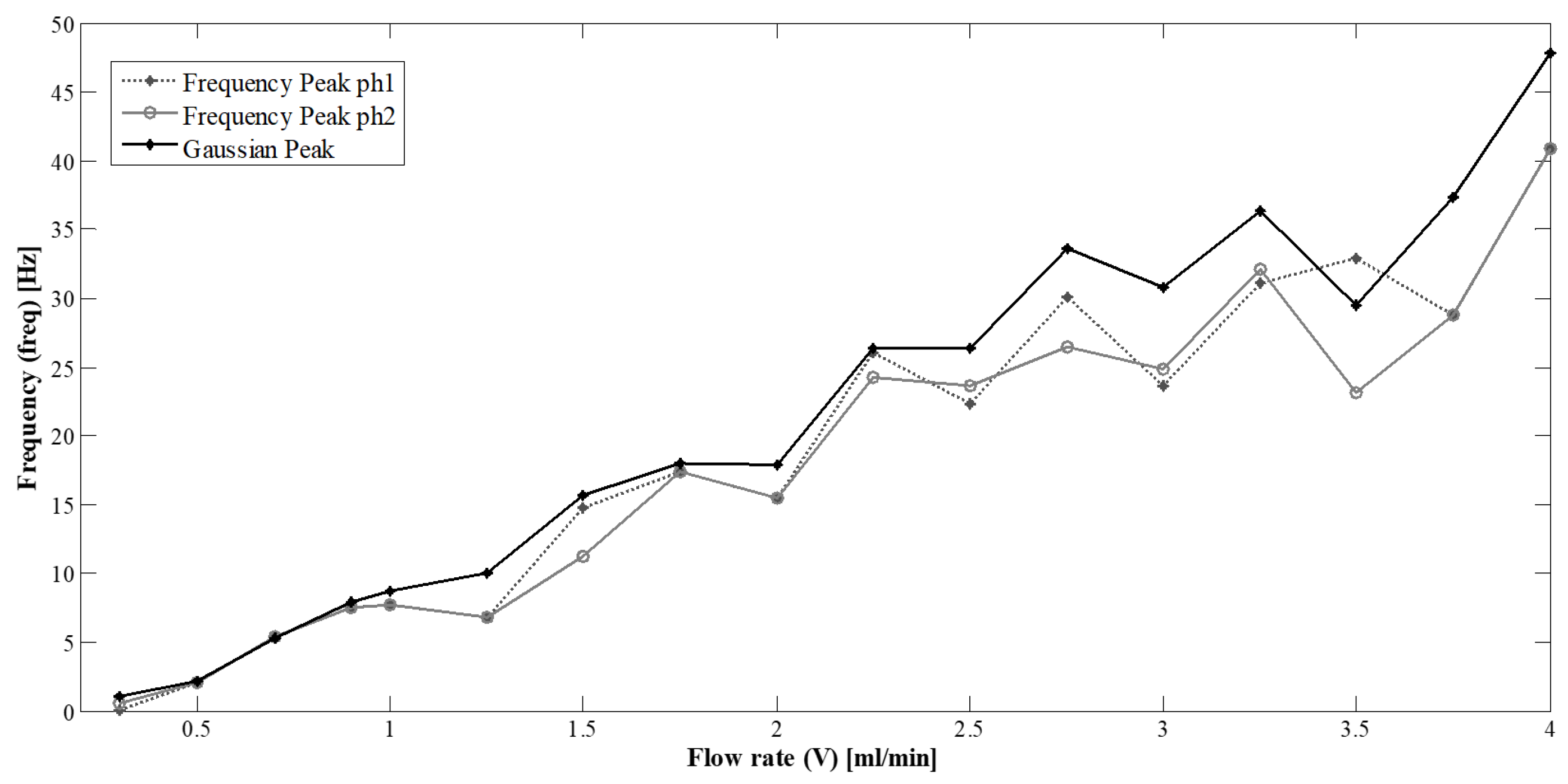
In the procedure proposed the profile of the spectrum of the optical signal was approximated with a Gaussian model for the automatic peak detection. Then this maximum in the spectrum, reported in Table 1 for each experiment, was used for the slug flow characterization, in terms of slower or faster slugs passage.
In Figure 4, the peaks computed by the Gaussian fitting (black solid line) are plotted and compared with the maximum spectrum peaks of the signals acquired by the two photo-diodes (black dashed lined and grey solid line) and extracted by visual inspection. Here we can note that the three trends are quite similar.
Consequently, this signal analysis approach based on the automatic peak detection of the dominant component in the spectral analysis proved to be valid tools for slugs flow continuous monitoring.
2.2. Transient Time in Slug Flows
To properly design a real-time control system, it is important to evaluate the transient time in the slug flow, so the time needed to modify the frequency of the slug flow by varying the input flow rate.
To investigate on this aspect an experiment was carried out in which the air and water input flow rates were set equal V = = and varied from to and then restored to zero. The micro-channel was initially filled by air. The optical signal acquired was recorded and analyzed in the frequency domain. Based on the slug flow characterization (see Figure 4) in steady condition the frequency of the slugs passage was expected at .
Figure 5 shows the signal changes in the different phases of the experiment:
- for the two input flow rates were set to zero , the signal detects the presence of air in the micro-channel;
- at the two input flow rates were set to , the signal initially detects only the presence of air till , then the signal switches showing clearly the presence of water till and finally the slug flow regime is established;
- at it was possible to detected a frequency of slugs passage stabilized to ;
- at the two input flow rates were restore to zero value, after the signal detects only the presence of air.
The , needed for the water to reach the micro-channel area where the process was analyzed, is correlated with the tubes and micro-channel lengths. Then was necessary to reach the slug regime [1] and to stabilize the slugs frequency.
Based on that it was possible to conclude that when the flow starts the total time needed to reach the steady condition is given by , instead for the slug frequency stabilization is necessary .
From the transient time computed for several conditions it was possible to observe that reaching the slug flow stabilization for a lower input flow rate requires a longer transient than for an higher input flow rate and moving from a lower to an higher flow rate, the transient time is larger than moving from an higher to a lower flow rate.
Taking these considerations into account and assuming the maximum transient time needed to reach the desired slug frequency equal to (when the process starts from a ), the optical signals acquired to perform a real-time slug flow control were analyzed in time windows of .
3. Feed-Forward Control System Design
The continuous monitoring and process control enable the maintenance of the frequency of the slugs passage with a limited range of variability, nevertheless the process nonlinearity correlated with the serpentine geometry and the two fluids interaction, as proved [4]. The feed-forward control system design proposed was tested in the case air-fluid interaction to guarantee the robustness of the control methodology established. Indeed the use of a compressible fluid as air increases the process complexity.
These microfluidic two-phase processes can be considered in the class of the two inputs and single output nonlinear dynamical systems where the inputs are the air and water input flow rates, while the output is related to the slug/air length or the inter-distance between slugs. Considering the frequency peak () as control parameter, we can design a control system in order to impose desired dynamics to the system in terms of desired slug frequency. Specifically, the experimental set-up of the feed-forward control system is shown in Figure 1, where the two algorithms implemented to control the syringe pumps actuation (Control Law) and for the automatic detection of the frequency of the slugs passage (Soft Sensor) were highlighted. The system designed was implemented in Labview.
3.1. Control Law Definition
The Figure 6 shows the schematic of the open loop control system for the microfluidic process (called ): the frequency parameter () is associated with a desired flow behavior and () is its actual value computed by the signal analysis procedure represented by the algorithm Soft Sensor. Given a control law to correlate the desired frequency of slug flow with the input flow rate it is possible to compute the new input flow rate (V = = ) to be imposed at the microfluidic system. The ideal condition is verified if .
Based on the results shown in Figure 4, the peak detected per experiment () was choosen as control parameter. The Control Law was defined by the linear interpolation (dashed line) of the data in zone-1 of Figure 7 considering the manipulation variable (V) along the y-axis and the control parameter () along the x-axis. In this plot, two zones can be seen: zone-1 (in the range of flow rate [–] mL/min and frequency [–] Hz) shows a more regular behavior and a more irregular part, named zone-2 (in the range of flow rate [–] mL/min and frequency [–] Hz). The authors decided to limit this study and implementation of the control law to the zone-1. The general equation of the linear fitting can be formalized by Equation (1):
where the manipulation variables of the control system are the two input flow rate assumed to be equal V = = that allow reaching the desired dynamics.
To validate the method proposed a subset of experiments in zone-1 was considered, in particular the range of flow rate [–] mL/min and frequency [–] Hz. The parameters of Equation (1) were, in this case, .
3.2. Labview Implementation
Based on the experimental set-up in Figure 1 the open loop platform developed in Labview includes a GUI and the four modules reported below:
- to manage the communication between the PC and the syringe pumps;
- to implement the Control Law;
- to manage the signals acquisition from the photodiodes;
- to implement the Soft Sensor for the analysis.
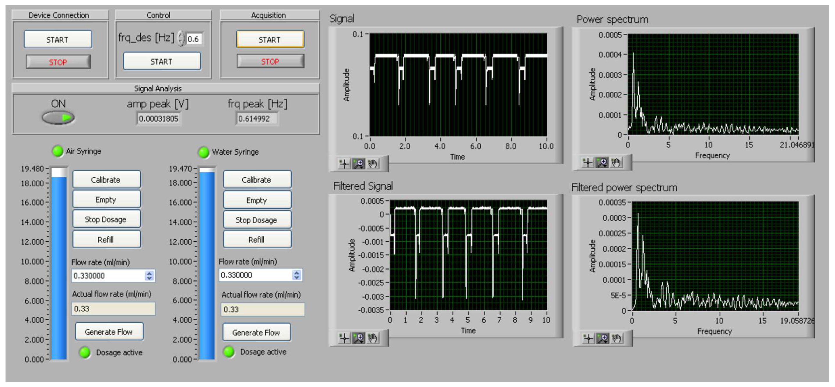
The GUI of the platform is presented in Figure 8. It consists of a section related to the pumps control and a section for the real-time monitoring of the raw and filtered signals and spectra. In the control section, it is possible to set the desired frequency of the slugs passage () and to read its actual value computed by the signal analysis procedure ().
In Figure 9 it is reported the Labview schematic for the module that implements the Control Law. The input parameter is the desired frequency () set in the GUI and the output parameters are the two new flow rates to be imposed to the pumps ( and ). The communication with the pumps is implemented by a Cetoni Nemesys ad-hoc block.
In Figure 10 it is reported the Labview schematic that implements signals acquisition and analysis modules.
The acquisition was set in the DAQ assistant block in order to acquire cyclically for the signal samples. The analysis module Soft Sensor includes the blocks for the signal filtering, the signal spectrum computation and the peak detection. It lasts less that and gives as output parameters . The filtering was implemented by a low-pass filter whose cut-off frequency was set to , to remove the noise of the power supply and the external lighting. Moreover, a band-stop filter was also used to remove the continuous frequency component. The system also provides blocks for saving the entire raw and filtered signals.
4. Results and Discussion
The desired frequency value is used to automatically set the syringe pump flow rate through the control law. The slug flow in the microchannel is checked each by the Soft Sensor implemented to control eventually variations on the flow velocity. In Figure 11, a real-time experiment is reported on, in which the value of the desired frequency was changed during the process evolution .
On the top of the figure the filtered signal, acquired during all the experiments and lasting , is reported. The three time windows (labeled with ) represents the trend of signal after the change of desired frequency value by the GUI. It is visible, at each change, that after a slight time interval of around the slug frequency passage is stabilized. The first portion of signal relative to the is plotted after the transition phase. Considering the signal segmented in three parts (each relative to the change of desired frequency) and neglecting the part of the signal relative to the transitory phase, the spectra were computed and plotted (lower part of Figure 11). The detected peaks are . Since the control is used in the open loop configuration, the results obtained can not be extremely precise and therefore a certain error was expected ().
5. Conclusions
A real-time platform implemented in Labview for the feed-forward control of the slug flow in micro-channels was implemented. The continuous monitoring and process control enable the maintenance of the frequency of the slug’s passage with a limited range of variability, nevertheless the process nonlinearity correlated with the serpentine geometry and the two fluids interaction. The feed-forward control system design proposed was tested in the case air-fluid interaction to guarantee the robustness of the control methodology established. Indeed the use of a compressible fluid as air increases the process complexity. One of the strengths of the results obtained is the possibility to detect and characterize the flow avoiding the used of dyes and invasive detection systems, not always suitable in biological context.
This approach takes the advantages of optical monitoring and on-line signal processing. In comparison with the standard passive and active microfluidic processes control strategies, it can be easily adapted in different experimental contexts and implemented for system on-chip control.
The experimental characterization of the slug flows by the frequencies of the slugs passage was obtained and used for the establishment of a control law. The experimental results obtained in the real-time slug control seems very promising for future development of this strategy. In the future, attention will be focused on the implementation of a more detailed control strategy in order to manage a wide range of dynamics: higher input flow rates and different values for the water and air input flow rates. Moreover, based on the complexity of the process, a closed loop control system could also be considered to reduce the frequency error increasing the performance of the control.
Author Contributions
The authors contributed equally to this work in conceptualization, methodology, software and writing.
Funding
This research was funded by FONDI PER LA RICERCA DI ATENEO- PIANO PER LA RICERCA 2016/2018.
Conflicts of Interest
The authors declare no conflict of interest.
References
- Tabeling, P. Introduction to Microfluidics; Oxford University Press: New York, NY, USA, 2005. [Google Scholar]
- Ribatski, G.; Wojtan, L.; Thome, J.R. An analysis of experimental data and prediction methods for two-phase frictional pressure drop and flow boiling heat transfer in micro-scale channels. Exp. Therm. Fluid Sci. 2006, 31, 1–19. [Google Scholar] [CrossRef]
- Schembri, F.; Bucolo, M. Periodic input flow tuning nonlinear two-phase dynamics in a snake microchannel. Microfluid. Nanofluidic 2011, 11, 189–197. [Google Scholar] [CrossRef]
- Schembri, F.; Sapuppo, F.; Bucolo, M. Experimental classification of nonlinear dynamics in microfluidic bubbles’ flow. Nonlinear Dyn. 2012, 67, 2807–2819. [Google Scholar] [CrossRef]
- Suk, J.W.; Cho, J.H. Capillary flow control using hydrophobic patterns. J. Micromech. Microeng. 2007, 17, 11–15. [Google Scholar] [CrossRef]
- Juncker, D.; Schmid, H.; Drechsler, U.; Wolf, H.; Wolf, M.; Michel, B.; De Rooij, N.; Delamarche, E. Autonomous microfluidic capillary sistem. Anal. Chem. 2002, 74, 6139–6144. [Google Scholar] [CrossRef] [PubMed]
- Unger, M.A.; Chou, H.P.; Thorsen, T.; Scherer, A.; Quake, S.R. Monolithic microfabricated valves and pumps by multilayer soft litography. Science 2000, 288, 113–116. [Google Scholar] [CrossRef] [PubMed]
- Fahrenberg, J.; Bier, W.; Maas, D.; Menz, W.; Ruprecht, R.; Schomburg, W.K. A microvalve system fabricated by thermoplastic molding. J. Micromech. Microeng. 1995, 5, 169–171. [Google Scholar] [CrossRef]
- Hosokawa, K.; Fuji, T.; Endo, I. Handling of picoliter liquid samples in a poly(dimethylsiloxane)-based microfluidic device. Anal. Chem. 1999, 71, 4781–4785. [Google Scholar] [CrossRef]
- Cairone, F.; Bucolo, M. Design of Control Systems for Two-Phase Microfluidic Processes. In Proceedings of the 24th Mediterranean Conference on Control and Automation (MED), Athens, Greece, 21–24 June 2016. [Google Scholar]
- Cairone, F.; Bucolo, M. Data-driven identification of two-phase microfluidic flows. In Proceedings of the 24th Mediterranean Conference on Control and Automation (MED), Athens, Greece, 21–24 June 2016. [Google Scholar]
- Cairone, F.; Gagliano, S.; Bucolo, M. Experimental study on the slug flow in a serpentine microchannel. Int. J. Exp. Therm. Fluid Sci. 2016, 76, 34–44. [Google Scholar] [CrossRef]
- Cairone, F.; Gagliano, S.; Carbone, D.C.; Recca, G.; Bucolo, M. Micro-optofluidic switch realized by 3D printing technology. Microfluid. Nanofluidics 2016, 20, 61–71. [Google Scholar] [CrossRef]
- Bruus, H. Theoretical Microfluidics; Oxford University Press: New York, NY, USA, 2008. [Google Scholar]
Figure 1.
Flow diagram of the experimental set-up: the two syringe pumps, the microfluidic channel, the opto-mechanical block and the optical acquisition. Two algorithms were developed: one to control the syringe pumps actuation (Control Law) and the other to detect the frequency of the slugs passage (Soft Sensor) in the straight part of the micro-channel.

Figure 2.
For the experiment with : (at the top) the trend of the optical signal after filtering and (at the bottom) its spectrum.
Figure 2.
For the experiment with : (at the top) the trend of the optical signal after filtering and (at the bottom) its spectrum.

Figure 3.
For the experiment with : (at the top) the trend of the optical signal after filtering and (at the bottom) its spectrum.
Figure 3.
For the experiment with : (at the top) the trend of the optical signal after filtering and (at the bottom) its spectrum.

Figure 4.
Experimental characterization of the slug flows by the frequencies of the slugs passage. Comparison among the peaks computed by automatic peak detection algorithm based on the Gaussian fitting (black solid line) and visual inspection of the spectra for the two photo-diodes acquisitions (black dashed lined and gray solid line).

Figure 5.
Trend of the optical signal acquired in the experiment to evaluate the transient in the slug flow: time needed to modify the frequency of the slug flow by varying the input flow rate. The air and water input flow rates were set equal V = = and varied from to and then restored to zero.
Figure 5.
Trend of the optical signal acquired in the experiment to evaluate the transient in the slug flow: time needed to modify the frequency of the slug flow by varying the input flow rate. The air and water input flow rates were set equal V = = and varied from to and then restored to zero.

Figure 6.
Feed-forward control scheme design.

Figure 7.
The peaks detected per experiment () are plotted in function of the manipulation variable (V). Two zones are distinguishable: the zone-1, that shows a regular behaviour and a more irregular part, named zone-2.
Figure 7.
The peaks detected per experiment () are plotted in function of the manipulation variable (V). Two zones are distinguishable: the zone-1, that shows a regular behaviour and a more irregular part, named zone-2.

Figure 8.
The GUI of the platform. It consists of a section related to the pumps control (on the left) and a section to monitor in real time the raw and the filtered signals and spectra (on the right).
Figure 8.
The GUI of the platform. It consists of a section related to the pumps control (on the left) and a section to monitor in real time the raw and the filtered signals and spectra (on the right).

Figure 9.
The Labview schematic for the module that implements the Control Law.

Figure 10.
The Labview schematic that implements signals acquisition and analysis modules Soft Sensor.
Figure 10.
The Labview schematic that implements signals acquisition and analysis modules Soft Sensor.

Figure 11.
Signal acquired by the Labview platform during a real-time experiment in which the value of the desired frequency was changed . The three time windows showing the different dynamics were highlighted and labelled with the values of the desired frequency. The three spectra were computed and the detected peaks are .


Table 1.
Experimental campaign: Flow rate (mL/min) and Frequency peak (Hz).
| Flow rate [mL/min] | 0.3 | 0.5 | 0.7 | 0.9 | 1.0 | 1.25 |
| Frequency [Hz] | 0.55 | 2.99 | 6.85 | 7.43 | 9.16 | 12.01 |
| Flow rate [mL/min] | 1.5 | 1.75 | 2.0 | 2.25 | 2.5 | 2.75 |
| Frequency [Hz] | 15.66 | 18.03 | 17.94 | 26.40 | 26.40 | 33.63 |
| Flow rate [mL/min] | 3.0 | 3.25 | 3.5 | 3.75 | 4.0 | |
| Frequency [Hz] | 30.84 | 36.34 | 29.46 | 37.32 | 47.81 |
Table 2.
Experimental campaign:Flow rate (mL/min) and Capillary Number.
| Flow rate [mL/min] | 0.3 | 0.5 | 0.7 | 0.9 | 1.0 | 1.25 |
| Capillary Number [] | 0.33 | 0.55 | 0.77 | 0.99 | 1.1 | 1.38 |
| Flow rate [mL/min] | 1.5 | 1.75 | 2.0 | 2.25 | 2.5 | 2.75 |
| Capillary Number [] | 1.65 | 1.93 | 2.2 | 2.48 | 2.76 | 3.03 |
| Flow rate [mL/min] | 3.0 | 3.25 | 3.5 | 3.75 | 4.0 | |
| Capillary Number [] | 3.31 | 3.58 | 3.83 | 4.16 | 4.41 |
© 2019 by the authors. Licensee MDPI, Basel, Switzerland. This article is an open access article distributed under the terms and conditions of the Creative Commons Attribution (CC BY) license (http://creativecommons.org/licenses/by/4.0/).
Share and Cite
MDPI and ACS Style
Gagliano, S.; Cairone, F.; Amenta, A.; Bucolo, M. A Real Time Feed Forward Control of Slug Flow in Microchannels †. Energies 2019, 12, 2556. https://doi.org/10.3390/en12132556
AMA Style
Gagliano S, Cairone F, Amenta A, Bucolo M. A Real Time Feed Forward Control of Slug Flow in Microchannels †. Energies. 2019; 12(13):2556. https://doi.org/10.3390/en12132556
Chicago/Turabian StyleGagliano, Salvina, Fabiana Cairone, Angelo Amenta, and Maide Bucolo. 2019. "A Real Time Feed Forward Control of Slug Flow in Microchannels †" Energies 12, no. 13: 2556. https://doi.org/10.3390/en12132556
Note that from the first issue of 2016, this journal uses article numbers instead of page numbers. See further details here.