Utilizing Asphalt Heat Energy in Finnish Climate Conditions


School of Technology and Innovations, University of Vaasa, 65101 Vaasa, Finland
*
Author to whom correspondence should be addressed.
Energies 2019, 12(11), 2101; https://doi.org/10.3390/en12112101
Submission received: 2 May 2019
/
Revised: 23 May 2019
/
Accepted: 24 May 2019
/
Published: 1 June 2019
(This article belongs to the Special Issue Low Carbon Energy Systems)
Abstract
:Geothermal energy is a form of renewable energy, which offers carbon-free solutions for heating and cooling spaces. This study evaluates the use of renewable asphalt heat energy in frozen ground conditions. Asphalt heat energy can be harnessed using a low-energy network, heat collection pipes and heat pumps. This study measured temperatures under the asphalt layer during a three-year period between 2014 and 2017. Measurements were made using a distributed temperature sensing method based on light scattering. Temperatures taken at four different depths under the asphalt (0.5 m, 1.0 m, 3.0 m and 10 m) are presented here. These temperatures are compared with that detected at the depth at which the temperature remains constant all year round. The temperature difference curve between 0.5 m depth and the constant soil temperature depth indicates that from April to October the soil at 0.5 m depth is warming and the temperature difference is positive, even as much as 18 °C. Instead, at the 3.0 m depth, the difference curve is smoother and it varies only from −5 to +5 °C. It is positive from June to November. The surface layer (0 m–1.0 m) is suitable for harvesting heat that can be stored in a deeper (1.5 m–3.0 m) purpose-built storage or in a bedrock heat battery. The calculated heat capacities indicate that asphalt energy, because of high temperatures, is a noteworthy renewable energy source.
1. Introduction
It is commonly accepted that climate change and global warming are serious issues that can be addressed by reducing greenhouse gas (GHG) emissions. According to Shrestha et al. [1], technological innovations and research to develop new solutions are essential to limit global warming. This is particularly true in developing countries, where there is still much to do. In Finland geothermal energy systems have been a popular heat source for new single family-houses in recent years. Heat pump systems most commonly use the bedrock, the ground and the air as a heat source. Even old houses and summer cottages are increasingly equipped with an air-to-air heat pump. Finns bought 76,000 heat pumps in 2018 [2]. People are prepared to invest in renewable sources, driven by the desire to cut their electricity and heating bills. At the same time, households are becoming more self-sufficient in heat energy. The Finnish government released its new national energy and climate strategy report in November 2016. According to that report, Finland will abandon the burning of coal for energy by 2030. Moreover, the aim is for at least 38% of the energy used by then to come from renewables. These targets mean that new approaches are needed in Finland to develop cost-effective applications with consumer-friendly prices for carbon-free energy systems. Studies of yearly savings and the payback period are made by Mallick et al. [3]. Geothermal energy, or more specifically the radiant energy emitted by the sun and stored in the upper layers of the earth, is a renewable energy source with a great potential in Finland.
There is a large amount of heat energy available in urban areas due to the proliferation of buildings, people, vehicles, concrete, asphalt and a lack of flora [4]. The air of an urban area is even several degrees warmer than in an adjacent rural area [5]. This urban heat island (UHI) effect is well-known, especially in the world’s big cities. The same phenomenon is found even in northern latitudes: the average yearly UHI intensity measured in the city of Turku, Finland, was 1.9 °C, compared with the rural area [6]. Not only is it apparent that there is much heat energy available in an urban area, but there is also a great demand for energy in the same area. It would be logical to use the energy near its birthplace.
Asphalt pavements, such as roads, car parks and pedestrian areas, are most prevalent in cities. They gather solar heat, and in doing so they bind a significant quantity of energy. Part of that energy conducts to underlying layers of asphalt. According to Qinwu & Mansour [7], the specific heat of asphalt concrete is 920 J/kg °C, measured as an average of several mixtures. Asphalt heat energy has already been utilized, for instance in England, where commercial solutions also exist [8]. The usual exploitation method entails a pipe network within an asphalt pavement or concrete slabs. The tubes are typically metallic, such as steel, aluminum or copper, but polymers like polyethylene or polyvinyle chloride (PVC) are also used. Pascual-Munoz et al. [9] have presented and tested a highly porous asphalt layer. This acts as a solar heat collector, removing the need for the tubes. It has excellent thermal efficiency, but needs further research to increase the flow rate. Different asphalt mixtures have also been studied by Dawson et al. [10]. The simulation of the thermal properties of asphalt pavements has been presented by Wang et al. [11].
The storage of heat is an important issue when considering the seasonal characteristics of asphalt energy. Borehole thermal energy storage (BTES) is a thick underground array of many shallow boreholes (35 m–120 m). For example, in the Drake Landing Solar Community, Canada, the BTES consists of 144 boreholes [12]. In Tianjin, China, Zhou et al. [13] have implemented an experimental asphalt-covered 12 m × 8 m field including heat-harvesting pipes and one vertical 120 m-deep heat storage. Heat collection was carried out during the summer 24 h per day, and that heat was used to warm the asphalt surface to prevent freezing for 24 h a day in winter. The heat harvesting in summer reduced the asphalt surface temperature and eliminated rutting [14]. Heat release during winter reduced the time that the asphalt pavement was frozen by 32%. The biggest BTES in Finland is located in the Sipoo logistics center, where there are 157 boreholes in a 310 m × 270 m area, with most of the boreholes being under the building [15].
The Finnish climate conditions are very hard when compared to China, Tianjin [13], but there is no permafrost like in Siberia. Here, the ground is frozen during the winter, even to a depth of 1.5 m [16]: hence, this study’s main objective is to assess if asphalt heat energy is at all viable in Finland.
The ground temperature remains relatively constant throughout the year beyond a certain depth because the seasonal variation of air temperature has no effect that far beneath the surface. For instance, in Cyprus this constant temperature is reached at a depth of 5.0 m [17]. In Finland, that depth is about 15 m [18]. According to Florides et al. [17] there are three main factors affecting the temperature distribution in the ground. First, there is the structure and physical properties of the ground. Second, there is the cover material on the ground surface (e.g., lawn, asphalt, etc.). The third factor is the climate conditions (air temperature, wind, solar radiation, air humidity and rainfall), because these have an influence on the ground temperature in the subsurface. It is primarily geothermal energy that influences the ground temperature below the depth at which the temperature is constant throughout the year.
Martinkauppi et al. [19] used a laboratory set-up to establish that different layers under the asphalt pavement stored the heat. A sample of asphalt pavement was heated with a bulb. After the heating ceased, the asphalt layer cooled down to the ambient temperature relatively rapidly, but the lowest layer, sand, stored some of the heat energy. That study indicated that different layers (asphalt, gravel, sand) had different thermal conductivities. During the heating period, the upper layer influenced the thermal behavior of what was below it, but its influence was not observed during the cooling.
The aim of this paper is to study ground temperatures below an asphalt-covered surface. Specifically, it focuses on temperatures at depths of 0.5 m to 3.0 m beneath the surface, because this is the portion of the ground most relevant to heat utilization in a low-energy network. These depths are also interesting in terms of seasonal heat energy storage. In this study, the depth of 0.5 m is found to retain appropriate temperature levels of up to 26 °C and to have positive temperature values for at least nine months per year. This layer is suitable for assembling heat collection pipes. This study shows that temperatures remain over 4 °C over the whole year at a depth of 3.0 m. That is why this layer might be suitable for seasonal heat storage, even in northern locations like Finland. Additionally, 3 m is still relatively shallow in civil engineering terms, so the installation of pipework at this depth is not onerous. The study also evaluates the temperature and the depth of constant soil temperature (CST) at the test site. Temperatures at different depths are compared with the CST. The temperatures under a lawn-covered field at a depth of 0.5 m are also presented as an example of a typical ground source heat potential under a non-asphalt field.
2. Materials and Methods
The measurement field for monitoring temperatures beneath the asphalt layer (five holes) and a similar lawn-covered field (five holes) was planned and installed by the research group for renewable energy in the University of Vaasa. The site for the measurement field was found at the University of Vaasa’s seaside campus area in the parking lot near the Gulf of Bothnia. In late autumn 2013, five holes were drilled through the asphalt-paved surface. Two holes went to a depth of 10 m, one to a depth of 5.0 m and two to a depth of 3.0 m (Figure 1). The temperature monitoring in the 10 m- and 5 m- holes was at a 1 m spatial resolution. However, it was possible to use a much smaller resolution in the 3.0 m-deep holes. The optical fiber inside the cable functions as a linear sensor. The cables were installed in the drilled holes. A more precise description of the measurement fields is written by Mäkiranta et al. [20,21]. The completed asphalt energy measurement field was finished with a new asphalt pavement and lawn field with grass seeds (Figure 2) in spring 2014.
The monthly mean air temperature data have been measured at the nearest weather station (less than 3 km) of the Finnish Meteorological Institute (see Table 1).
The distance between the asphalt and lawn measurement fields is no more than about 200 m, which ensures that the solar and other weather conditions are similar.
The temperature monitoring beneath the asphalt cover was made by using the distributed temperature sensing (DTS) method. This method entails an optical fiber inside an armored cable in each hole. The optical fiber functions as a linear sensor, and the DTS measurement device (Sensornet Oryx) observes the temperatures along the fiber. Short pulses of laser light are emitted by the DTS measurement device to illuminate the glass core of the optical fiber. Part of the incident light pulse is backscattered while it moves along the core of fiber. The intensity of these backscattered bands is acquired by the DTS measurement device. The device estimates the temperatures based on the temperature dependent part of the scattering, Raman scattering [22]. The temperature accuracy of the Oryx device is ±0.5 °C. The optical fibers in the 3 m-deep holes were spiral-wrapped around a measurement pipe, improving the resolution in these shallow holes to 0.03 m. Spiral-wrapping was not used in the 10 m- and 5 m-holes, so their spatial resolution was 1 m.
During the three-year measurement period of 2014–2017, the temperatures were monitored at several depths, from a 0.2 m up to a 10 m depth. The most interesting layer, in terms of the asphalt heat collection, was observed to be at 0.5 m. The layer for optimal seasonal storage was found to be at 3.0 m. The temperatures at an intermediate depth of 1.5 m are also presented for comparative purposes and to verify the suitability of the two other layers.
The measurements were made once per month, except in July and August when they were made at two-week intervals (Table 2). The long intervals between the measurements were possible because temperature changes in the soil were relatively slow. Each measurement action lasted 10 min, during which the DTS device made two measurements per minute per channel. The total temperature data consist of 20 measurements per channel. Figure 3, Figure 4, Figure 5, Figure 6, Figure 7 and Figure 8 graph the average temperatures of eight measurements on each measurement date. The measurement field includes two 3.0 m-deep holes.
In respect to the lawn-covered field, this study only includes data from the period of April 2014–December 2015. Problems with splice connections caused a temporary interruption in the measurements on that field.
3. Results
Figure 3, Figure 5 and Figure 6 show the temperature data taken at depths of 0.5 m, 1.5 m and 3.0 m in the two 3.0 m-deep holes in the asphalt field. For a comparison, the temperatures at the depth of 0.5 m in the lawn-covered field are presented in Figure 4. Figure 3 represents the monthly mean air temperatures measured during April 2014–March 2017 [17]. In each of the three years of the monitoring period, either July or August was the warmest month, and either January or February was the coldest.
The timetable of the measurements is converted into the number of days between two measurement actions. The cumulative time t [day] since the beginning of the measurements is also presented (Table 2).
The temperatures measured at 0.5 m depth under the asphalt layer show a seasonal variation from −3.9 °C to 26.0 °C (Figure 3). The graph shows that the soil was frozen each year from January to as late in the year as March. A temperature increase of ten degrees can be seen during a one-and-a-half-month period right at the beginning of the study, from April to May 2014. Finland had especially warm weather in July 2014, which can be seen as a temperature peak under the asphalt pavement throughout that month. In contrast, 2015’s summer was cooler, and the warming of the soil was slower. In that year, the highest soil temperature (19.7 °C) at a depth of 0.5 m under the asphalt layer was not measured until the end of August. In 2016, the highest value, 19.4 °C, was measured at the beginning of August.
The data from both measurement holes are almost identical throughout the whole period of 2014–2017 for both the asphalt-covered (Figure 3) and lawn-covered areas (Figure 4).
The temperatures at 0.5 m under the lawn-covered field (Figure 4) were lower in the summer than in the asphalt-covered area. (Figure 3): summer 2014: 20 °C -> 26 °C, summer 2015: 16 °C -> 20 °C. With the exception of the temperature values in Figure 3 and Figure 4, the curves have only small differences in the shape of the temperature maximum.
The temperature graph at the depth of 1.5 m (Figure 5) under the asphalt layer demonstrates that the seasonal temperature variation was about 13–14 °C. The lowest temperatures were monitored from January to April, when they varied from 2.4 °C to 4.8 °C. The highest temperatures were in August of each year. At this intermediate depth of 1.5 m, the temperatures were quite low during winter and at the beginning of spring. Once again, the data from both measurement holes are almost identical throughout the whole period of 2014–2017.
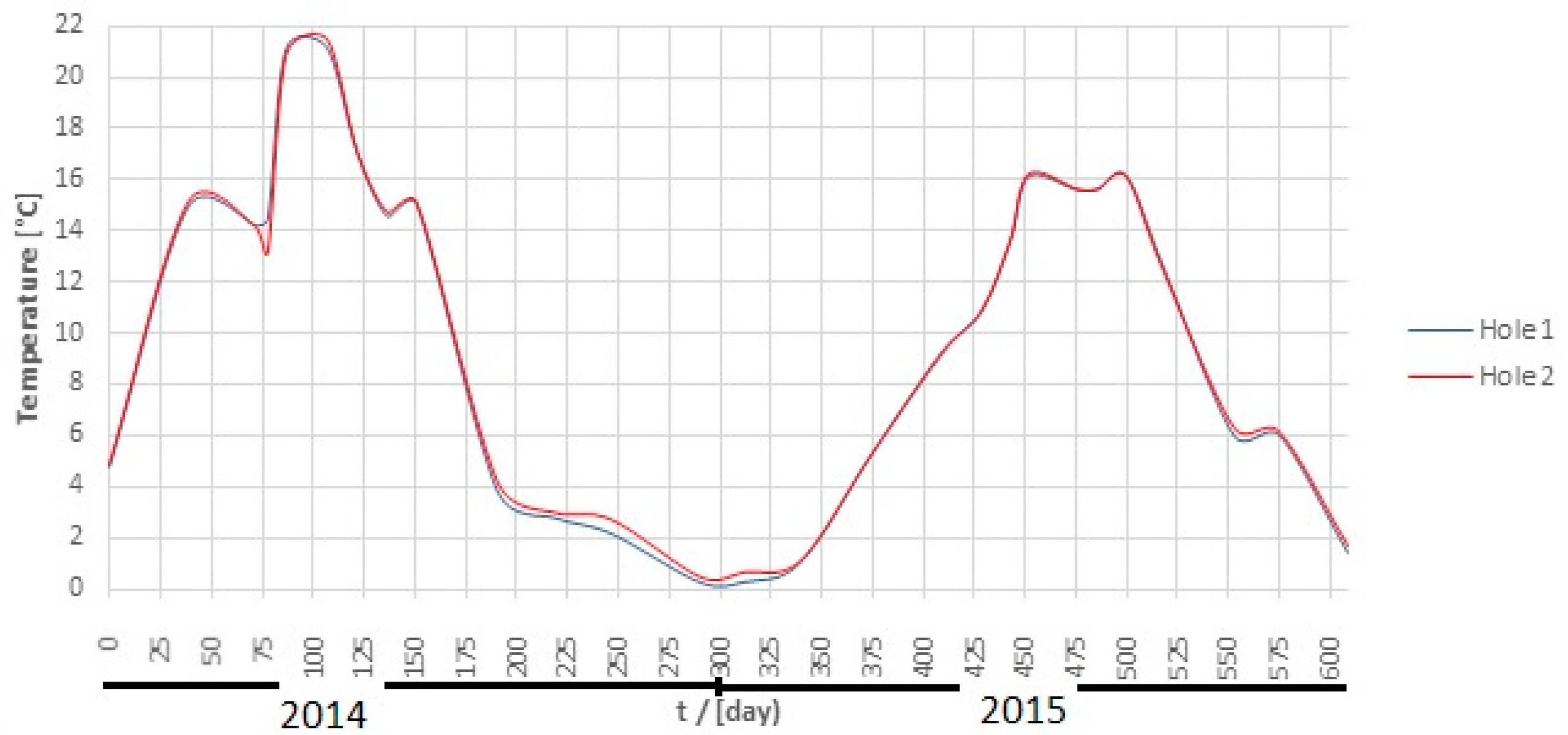
Figure 6 indicates the temperatures at a depth of 3.0 m under the asphalt layer during the three-year period. The temperatures vary from 2.9 °C (April) to 13.1 °C (August and September). The seasonal variation of about 8–10 °C is smaller than at the two shallower depths, and this soil layer has no frost. There is some variation between the two holes’ temperature data, particularly in the period of 2015–2017. The distance between the holes is only about 4.5 m, but the soil moisture and sand content may vary at a depth of 3.0 m. The heat capacity of the soil material at these two measurement points is apparently different.
Temperature Variation in Different Layers and the Constant Soil Temperature (CST) Layer
The seasonal variation in the soil temperature diminishes as the depth increases until a point is reached where the seasonal variation of the air temperature has no effect on the soil temperature (Figure 7). That depth was observed to be 10 m in this study. The temperature at this point was measured at a constant of 8 ± 1 °C throughout the year.
This stabilization of the temperature to 8 °C at a depth of 10 m, regardless of the season, was also noticed in the periods of April 2015–March 2016 and April 2016–March 2017. Figure 7 shows that from May to September the upper layers were warmer than the deeper layers; and from October to April the upper layers were cooler than the deeper layers. The heat transfer occurred from beneath, toward the asphalt layer.
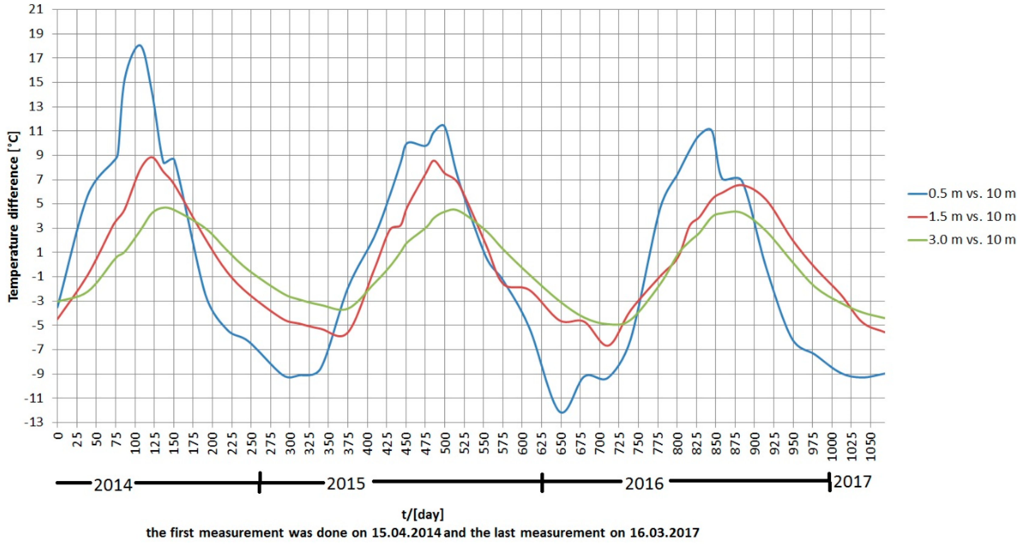
The difference curves in Figure 8 indicate the seasonal variation of the temperatures compared to the CST in different depths under the asphalt throughout the three-year study. It also shows the differences in the heat conduction speed between the studied layers. For example, it can be seen that the maximum temperature difference at 1.5 m occurred more than two weeks later than at 0.5 m. The variation in the temperature differences smoothen from the surface to the deeper layers. At a 0.5 m depth, the difference varies by even 30 °C, while at a 3.0 m depth the variation is less than 10 °C.
An estimation of the amount of heat energy E [kJ or kWh] in a 50 cm-thick soil layer including the asphalt cover (total volume 1 m·1 m·0.5 m = 0.5 m3), can be calculated
where E is the stored energy in the soil layer, m is the mass of the soil layer, c is the specific heat capacity (Table 3) and ΔT is the temperature difference of the two compared stages, ρ is the density of the soil layer (Table 3) and V is the volume of the soil layer.
E = m c ΔT, m = ρ·V
Thickness of the asphalt layer: 0.07 m; V = 0.07 m3; ma = 168 kg.
Thickness of the gravel (1/3) and sand layer (2/3) is 0.43 m; Vg+s = 0.43 m3; Vg = 0.14 m3; Vs. = 0.29; mg = 235 kg; ms = 771 kg.
A theoretical maximum for the available heat energy amount in the asphalt-covered layer (Vtot = 0.5 m3) is 20,785 kJ ≈ 5.77 kWh when soil types are dry and ΔT = 18 °C (the annual maximum temperature of the depth is 22 °C and the lowest permitted temperature chosen for the soil is 4 °C).
The estimation of the heat energy amount (heat capacity) in the 50 cm thick soil layer including the lawn cover (total volume 1 m ×·1 m·× 0.5 m = 0.5 m3; soil properties (Table 4)):
E = m c ΔT, m = ρ·V
Thickness of the soil layer: 0.1 m; Vs. = 0.1 m3; ms = 160 kg.
Thickness of the clay layer is 0.4 m; Vc = 0.4 m3; mc,dry = 640; mc,wet = 704 kg.
A theoretical maximum for the available heat energy amount in the lawn-covered layer (Vtot = 0.5 m3) is 10,368 kJ ≈ 2.88 kWh when soil is dry and ΔT = 15 °C (the annual maximum temperature of the depth is 19 °C and the lowest permitted temperature chosen for the soil is 4 °C). A theoretical maximum for the available heat energy amount in the lawn-covered layer (Vtot = 0.5 m3) is 22,138 kJ ≈ 6.15 kWh when soil is wet and the clay moisture is at 50% (average moisture ratio in Finland [28]).
A new, low-energy, single family house (140 m2, 4 persons) in Finland consumes 12,400 kWh annually for heating on average. This equates to 33.90 kWh per day [28].
To cover this average heating demand for a single family house for one day, an area of 5.9 m2 is needed in the asphalt-covered field. In the case of the lawn-covered field, an area of 11.8 m2 is needed if the soil types are dry, but only 5.5 m2 is sufficient if the soil types are wet. These calculations depend on the chosen values of the variables.
4. Discussion and Conclusions
The temperatures at a depth of 0.5 m (Figure 3) under the asphalt layer are very promising for heat collection from May until as late in the year as September. The temperatures at that depth are 10–14 °C in May, rising to 26 °C in July and then falling back to 15–16 °C in September. This five-month period from late spring to autumn can be utilized to collect heat. However, due to a low heating demand in summer, even in Finland, it is desirable that heat collected during that period can be stored. A purpose-designed storage deeper under the asphalt, or a bedrock heat battery, could act as a seasonal thermal energy storage (STES). It would be loaded by the asphalt energy during the summer and then the heat would be exploited at cooler times of the year. This asphalt heat energy would be suitable for hybrid energy systems. Asphalt heat can be used to cut off the peak loads of heat energy consumption during winter. Similarly, solar and wind energy are intermittent energy forms that require supplementary elements in order to produce a functional hybrid energy system.
The DTS measurement method was found to be reliable and accurate. There were two measurement holes with similar installations, and both sites gave very similar results without any interruptions (see Figure 2, Figure 3 and Figure 4).
At a depth of 1.5 m, the temperature falls below 3 °C. During a hard and snowless winter, this layer is frozen, at least in northern Finland. In contrast, 3 m below the asphalt layer the ground remains unfrozen year-round. The temperatures there range from 4 to 12 °C, which is eminently suitable for using asphalt heat continuously for heating or cooling houses. A low-energy system using asphalt energy as the heat source should comprise vertically installed heat-collection pipes and a heat pump. The heat carrier fluid in the pipeline gathers the heat energy, which is mainly emitted by the sun, absorbed by the asphalt and conducted through the soil.
Because of the large usable temperature difference, asphalt energy under the asphalt cover is a noteworthy energy source alongside other ground heat sources. Future research should also investigate the potential and implementation of heat storage to complement asphalt energy. Such a study should evaluate the properties of the asphalt layer and sand layer in capturing and storing energy, and, crucially, the amount of energy returned from the heat storage. In the future, asphalt pavements could act as passive solar collectors in urban areas.
Author Contributions
A.M.; investigation, original draft preparation, writing—review and editing, data curation; E.H.; supervision, funding acquisition, resources, writing—review and editing.
Funding
This research received external funding from Groove program of TEKES (Business Finland).
Acknowledgments
We would like to express thanks to the University of Vaasa for convenient research platform for these new kinds of measurements and the supervising group from the industry.
Conflicts of Interest
The authors declare no conflict of interest.
References
- Shrestha, S.; Babel, M.S.; Pandey, V.P. Climate Change and Water Resources; CRC Press: Boca Raton, FL, USA, 2014; pp. 69–80. [Google Scholar]
- The Finnish Heat Pump Association (SULPU). Available online: https://www.sulpu.fi/documents/184029/0/SULPU%20Press%20release%201.2019_en%20with%20picture%20.pdf (accessed on 28 January 2019).
- Mallick, R.; Carelli, J.; Albano, L.; Bhowmick, S.; Veeraragavan, A. Evaluation of the potential of harvesting heat energy from asphalt pavements. Int. J. Sustain. Eng. 2011, 2011. 4, 164–171. [Google Scholar] [CrossRef]
- Allen, A.; Dejan, M.; Sikora, P. Shallow gravel aquifers and the urban ‘heat island’ effect: a source of low enthalpy geothermal energy. Geothermics 2003, 32, 569–578. [Google Scholar] [CrossRef]
- Zhu, K.; Blum, P.; Ferguson, G.; Balke, K.-D.; Bayer, P. The Geothermal potential of urban heat islands. Environ. Res. Lett. 2010, 5, 1–6. [Google Scholar] [CrossRef]
- Suomi, J. Characteristics of Urban Heat Island (UHI) in a High-Latitude Coastal City—A Case Study of Turku. SW Finland. Annales Universitatis Turkuensis A II: Biologica. Geographica. Geologica. 2014. Available online: http://urn.fi/URN:ISBN:978-951-29-5912-9 (accessed on 28 January 2019).
- Xu, Q.; Solaimanian, M. Modeling temperature distribution and thermal property of asphalt concrete for laboratory testing applications. Constr. Build. Mater. 2010, 24, 487–497. [Google Scholar] [CrossRef]
- ICAX ltd. Asphalt Solar Collector. Available online: https://www.icax.co.uk/asphalt_solar_collector.html (accessed on 22 May 2019).
- Pascual-Munoz, P.; Castro-Fresno, d.; Serrano-Bravo, P.; Alonso-Estebanez, A. Thermal and hydraulic analysis of multilayered asphalt pavements as active solar collectors. Appl. Energy 2013, 111, 324–332. [Google Scholar] [CrossRef] [Green Version]
- Dawson, A.R.; Dehdezi, P.K.; Hall, M.R.; Wang, J.; Isola, R. Enhancing thermal properties of asphalt materials for heat storage and transfer applications. Road Mater. Pavement Des. 2012, 13, 784–803. [Google Scholar] [CrossRef] [Green Version]
- Wang, H.; Wu, S.; Chen, M.; Zhang, Y. Numerical simulation on the thermal response of heat-conducting asphalt pavements. Phys. Scr. 2010, 2010. [Google Scholar] [CrossRef]
- Mesquita, L.; McClenahan, D.; Thornton, J.; Carriere, J.; Wong, B. Drake Landing Solar Community: 10 years of operation. ISES Solar World Congress 2017. IEA SHC International Conference on Solar Heating and Cooling for Buildings and Industry. Available online: http://proceedings.ises.org (accessed on 10 April 2019). [CrossRef]
- Zhou, Z.; Wang, X.; Zhang, X.; Chen, G.; Zuo, J.; Pullen, S. Effectiveness of pavement-solar energy system—An experimental study. Appl. Energy 2015, 138, 1–10. [Google Scholar] [CrossRef]
- Mallick, R.B.; Chen, B.-L.; Bhowmick, S. Harvesting energy from asphalt pavements and reducing the heat island effect. Int. J. Sustain. Eng. 2009, 2, 214–228. [Google Scholar] [CrossRef]
- Korhonen, K.; Leppäharju, N.; Hakala, P.; Arola, T. Simulated temperature evolution of large BTES—Case study from Finland. In Proceedings of the IGSHPA Research Conference 2018, Stockholm, Sweden, 18–20 September 2018; pp. 482–490. [Google Scholar]
- Finnish Environment Institute. Depth of ground frost. Available online: URL:http://wwwi3.ymparisto.fi/i3/paasivu/ENG/Routa/Routa.htm (accessed on 28 January 2019).
- Florides, G.; Kalogirou, S. Ground heat exchangers—A review of systems, models and applications. Renew. Energy 2007, 32, 2461–2478. [Google Scholar] [CrossRef]
- Leppäharju, N. Kalliolämmön hyödyntämiseen vaikuttavat geofysikaaliset ja geologiset tekijät. Pro Gradu tutkielma; University of Oulu: Oulu, Finland, 2008; Available only in Finnish. [Google Scholar]
- Martinkauppi, J.B.; Mäkiranta, A.; Kiijärvi, J.; Hiltunen, E. Thermal Behavior of an Asphalt Pavement in the Laboratory and in the Parking lot. Sci. World J. 2015, 2015, 7. [Google Scholar] [CrossRef] [PubMed]
- Mäkiranta, A.; Martinkauppi, B.; Hiltunen, E. Design of Asphalt Heat Measurement in Nordic Country. In Proceedings of the SDEWES2016, Lisbon, Portugal, 4–9 September 2016. ISSN (printed) 1847-7178. [Google Scholar]
- Mäkiranta, A.; Martinkauppi, B.; Hiltunen, E. Thermal profiles under an asphalt and lawn covered fields. In Proceedings of the SDEWES2017, Dubrovnik, Croatia, 4–8 October 2017. ISSN (printed) 1847-7178. [Google Scholar]
- Abhisek, U.; Braendle, H.; Krippner, P. Distributed Temperature Sensing: Review of Technology and Applications. IEEE Sens. J. 2012, 12, 885–892. [Google Scholar]
- Finnish Meteorological Institute FMI. Monthly average air temperature data 2014–2017; Finnish Meteorological Institute FMI: Klemettilä, Vaasa, Finland.; Available online: https://ilmatieteenlaitos.fi/havaintojen-lataus#!/ (accessed on 28 January 2019).
- Valtanen, E. Handbook of Math and Physics. Matematiikan ja fysiikan käsikirja. (in Finnish) 2.painos; Genesis-kirjat Oy: Jyväskylä, Finland, 2007; ISBN 978-952-9867-28-8. [Google Scholar]
- Engineering toolbox. Densities and heat capacities of materials. Available online: https://www.engineeringtoolbox.com (accessed on 12 February 2019).
- Blocon, A.B. EED Earth Energy Designer—Vertical Borehole Design Program for PC; BLOCON SWEDEN: Lund, Sweden, 2018. [Google Scholar]
- Ronkainen, N. Properties of Finnish soil types. In Finland’s Environment 2/2012; Only in Finnish; Finnish Environment Institute: Helsinki, Finland, 2012; Available online: https://helda.helsinki.fi/handle/10138/38773 (accessed on 10 April 2019).
- Motiva Consumer Guidance. Calculator to compare the heating systems. Only in Finnish. Available online: http://lammitysvertailu.eneuvonta.fi/ (accessed on 12 February 2019).
Figure 1.
The measurement arrangements of the cables (left) and the geometrical positions of the holes (right) in the asphalt field. The same kind of independent measurement configuration was installed under the lawn.
Figure 1.
The measurement arrangements of the cables (left) and the geometrical positions of the holes (right) in the asphalt field. The same kind of independent measurement configuration was installed under the lawn.

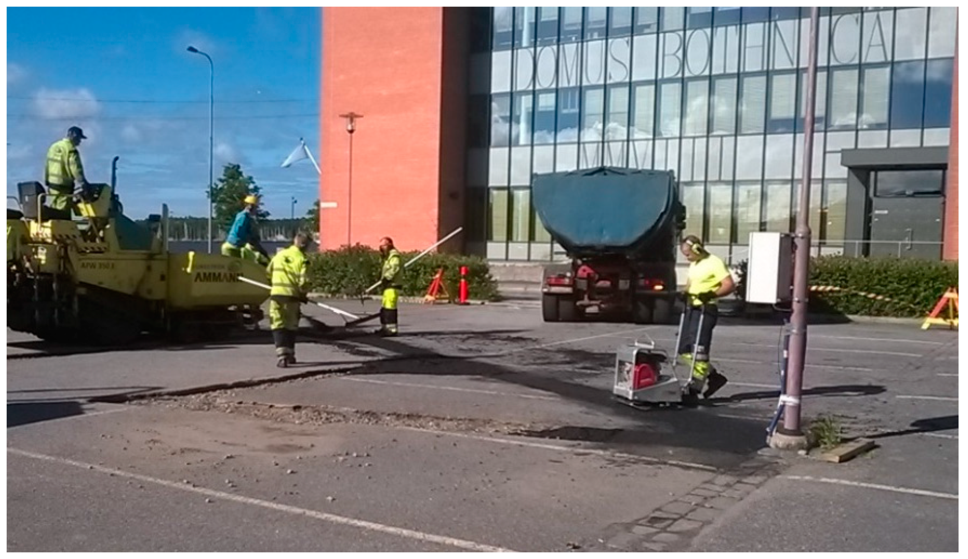
Figure 2.
The measurement field receives asphalt pavement after drilling and digging.

Figure 3.
The temperature at a 0.5 m depth under the asphalt layer in two different holes, and the average air temperature of the month [23].
Figure 3.
The temperature at a 0.5 m depth under the asphalt layer in two different holes, and the average air temperature of the month [23].

Figure 4.
The temperatures in the soil at a 0.5 m depth under the lawn cover.

Figure 5.
The temperatures in the soil at a 1.5 m depth under the asphalt layer.

Figure 6.
Temperatures in the soil at a 3.0 m depth under the asphalt layer.

Figure 7.
The temperatures in different layers from 0.5 m to 10 m are monitored at one hole. The temperatures vary between 7.4 °C and 8.8 °C at a depth of 10 m.
Figure 7.
The temperatures in different layers from 0.5 m to 10 m are monitored at one hole. The temperatures vary between 7.4 °C and 8.8 °C at a depth of 10 m.

Figure 8.
The difference curves compared with each other at 0.5 m, 1.5 m and 3.0 m.


Table 1.
The monthly mean air temperatures [°C] measured during April 2014–March 2017 at the weather station of the Finnish Meteorological Institute [23].
Table 1.
The monthly mean air temperatures [°C] measured during April 2014–March 2017 at the weather station of the Finnish Meteorological Institute [23].
| Jan. | Feb. | Mar. | Apr. | May. | Jun. | Jul. | Aug. | Sep. | Oct. | Nov. | Dec. | |
|---|---|---|---|---|---|---|---|---|---|---|---|---|
| 2014 | 4.2 | 9.3 | 12.6 | 20.0 | 16.5 | 11.5 | 5.0 | 1.0 | −0.7 | |||
| 2015 | −3.1 | −0.2 | 0.1 | 4.0 | 8.4 | 12.1 | 15.2 | 16.5 | 12.1 | 5.9 | 3.9 | 1.2 |
| 2016 | −9.7 | −2.3 | 0.1 | 3.3 | 11.0 | 14.0 | 17.2 | 14.6 | 11.9 | 4.0 | −1.1 | −0.5 |
| 2017 | −2.3 | −3.9 | −0.3 |
Table 2.
The timetable for the measurements, between April 2014 and March 2017; the number of days between two measurements (Δt), and the time t [day] since the beginning of the measurements (used as the x-axis in Figure 3, Figure 4, Figure 5 and Figure 6).
| Year | Date | Δt | t [Day] | Year | Date | Δt | t [Day] |
|---|---|---|---|---|---|---|---|
| 2014 | 16 April | 0 | 0 | 2015 | 27 August | 14 | 500 |
| 23 May | 39 | 39 | 14 September | 18 | 518 | ||
| 25 June | 33 | 72 | 19 October | 35 | 553 | ||
| 1 July | 6 | 78 | 10 November | 22 | 575 | ||
| 10 July | 9 | 87 | 14 December | 34 | 609 | ||
| 30 July | 20 | 107 | 2016 | 22 January | 39 | 648 | |
| 14 August | 15 | 122 | 23 February | 32 | 680 | ||
| 29 August | 15 | 137 | 24 March | 31 | 711 | ||
| 12 September | 14 | 151 | 22 April | 29 | 740 | ||
| 22 October | 40 | 191 | 30 May | 38 | 778 | ||
| 19 November | 28 | 219 | 22 June | 23 | 801 | ||
| 17 December | 28 | 247 | 7 July | 15 | 816 | ||
| 2015 | 30 January | 44 | 291 | 20 July | 13 | 829 | |
| 20 February | 21 | 312 | 5 August | 16 | 845 | ||
| 20 March | 28 | 340 | 18 August | 13 | 858 | ||
| 24 April | 35 | 375 | 13 September | 26 | 884 | ||
| 28 May | 34 | 409 | 14 October | 31 | 915 | ||
| 17 June | 20 | 429 | 16 November | 33 | 948 | ||
| 1 July | 14 | 443 | 16 December | 30 | 978 | ||
| 10 July | 9 | 452 | 2017 | 18 January | 33 | 1011 | |
| 3 August | 24 | 476 | 15 February | 28 | 1039 | ||
| 13 August | 10 | 486 | 16 March | 29 | 1068 |
| Soil Type | Specific Heat Capacity [kJ/kg·°C] | Density [kg/m3] |
|---|---|---|
| Asphalt | 0.92 | 2400 |
| Gravel | 1.50 (dry) | 1680 (dry) |
| Sand | 0.84 (dry, 20 °C) | 2660 |
© 2019 by the authors. Licensee MDPI, Basel, Switzerland. This article is an open access article distributed under the terms and conditions of the Creative Commons Attribution (CC BY) license (http://creativecommons.org/licenses/by/4.0/).
Share and Cite
MDPI and ACS Style
Mäkiranta, A.; Hiltunen, E. Utilizing Asphalt Heat Energy in Finnish Climate Conditions. Energies 2019, 12, 2101. https://doi.org/10.3390/en12112101
AMA Style
Mäkiranta A, Hiltunen E. Utilizing Asphalt Heat Energy in Finnish Climate Conditions. Energies. 2019; 12(11):2101. https://doi.org/10.3390/en12112101
Chicago/Turabian StyleMäkiranta, Anne, and Erkki Hiltunen. 2019. "Utilizing Asphalt Heat Energy in Finnish Climate Conditions" Energies 12, no. 11: 2101. https://doi.org/10.3390/en12112101
Note that from the first issue of 2016, this journal uses article numbers instead of page numbers. See further details here.