1. Introduction
Smart energy systems can support the mitigation of climate change cost-effectively. Mathiesen et al. [
1] describe smart energy systems as the ultimate concept of deploying 100% renewable energy sources to the energy system. Although district heating (DH) is a mature technology and combined heat and power (CHP) is deemed as a conventional energy source, there is still demand for operating them to their full extent because of their indispensable role in the energy sector. Therefore, DH systems with renewables and novel thermal energy storage (TES) technologies is a promising solution for reaching the 100% renewable society.
Currently, more than half of the total energy use by the Finnish residential and service sectors stems from space heating and hot water demands, accounting for 80 TWh in 2017 [
2]. Around 46% of this energy is covered by DH systems [
3]. One of the main challenges in the operation of DH systems is the occasionally significant variations in heat load, which result in part-load operation and frequent start-ups and stops for heat generation units [
4]. Hence, integrating TES systems into DH networks can improve the balance between the heat load and supply, thereby decreasing the demand for high-cost marginal generation.
The use of information and communication technologies (ICT) to improve the operation of DH networks and to automatically shape energy demand has been researched across Europe [
5,
6,
7,
8,
9]. This has been defined as demand-side management, which is an umbrella term for different building-side management strategies including peak clipping, valley filling and demand response (DR) [
10]. DR has been defined in this paper as programs designed to encourage users or building owners to allow short-term modifications in energy demand in response to a trigger initiated by the local energy company. This can comprise short reductions in energy demand, demand shifting and peak load reduction. DR can be seen as a decentralized TES, as heat is stored within the construction and comfort is retrained though the thermal inertia of the building [
11].
DR has been studied utilizing various kinds of building simulation tools [
5,
12,
13]. Difs et al. [
12] concluded that DR is an optimal energy efficiency measure. However, their study concludes that DR is beneficiary mainly during intermediate seasons, i.e., during large daily outdoor temperature variations. This gives a relatively short time frame for DR. Dréau and Heiselberg [
5] conclude that the control potential of the thermal mass of the building varies greatly according to both building-dependent and weather-dependent factors. The paper describes also how a building can provide flexibility to the thermal grid.
Through successful simulations and the availability of commercial control devices, DR has been also studied in the DH context in field tests [
7,
14,
15], demonstrating that ICT, including Internet of Things and cloud computing, are technically viable with commercial potential. This has been also concluded by Zhang et al. [
16]: the technological readiness of digital transition at the building level has been already demonstrated. However, the technology readiness level is not similar at all hierarchy levels. The paper denotes that technology readiness level of digital transition at district and city level is still below technology development.
The timing between DH production and consumption can be balanced from the DH operator side as well, utilizing centralized hot water tanks (HWTs). HWTs are typically situated close to power plants [
17] since electricity and DH sectors are linked through CHP plants and large heat pumps. Sometimes heat demand and high electricity prices (i.e., hours at which CHP plant receives high revenues from electricity sales) do not occur at the same time. Heat storage units, such as HWTs, may help balance the timing between demand and supply [
18]. Therefore, in this paper, the profitability of combining DR with an HWT is examined.
The research investigates how DR performs in DH networks and the effect of additional utilization of HWTs when performing DR. Romanchenko et al. [
19] have compared these techniques with the result that when both storage types have the same maximal capacity, the frequency and rate of charging and discharging is the same for both, although HWT can store more than double the amount of heat in a year due to its ability to store heat also on the medium-term [
19]. This results in the HWT conferring more than twice the savings, but as DR can have significantly lower investment costs, the economic comparison cannot be extrapolated.
DR and HWT differ also from the stakeholders’ perspective. The decisions related to the operation of HWT are made exclusively by the DH system operator, whereas the utilization of DR requires the involvement of customers. The customers can be triggered through a change in energy price but it is probably not activated if the thermal comfort is jeopardized [
14].
Several studies that have modelled district energy systems, including those that incorporate TES, are discussed in a review paper of Sameti and Haghighat [
7]. They noticed that the objective function optimizes typically amongst others carbon emissions, production, revenue, operation costs and fuel costs. Often, only one type of TES is simulated. Moreover, the annual peak heat load was only slightly decreased if energy conservation was not encompassed. Guelpa et al. [
8] present a physical simulation tool with the objective of minimizing the primary energy consumption at the thermal plants. In that model, the schedules of the buildings heating systems are modified to meet system demand. Additionally, constraints for indoor temperature variations are introduced in order to archieve acceptable comfort levels.
In addition to the utilization of just one TES type, previous research has typically utilized one approach on modeling DR, i.e., either from the building perspective of the grid perspective. When the focus is on the grid characterization, building models do not often capture the fine dynamics of buildings. On the other hand, when focusing on the building side, the grid optimizations remain usually at the parcel level. Kontu et al. [
7] determined that implementing DR as TES has a minor benefit, less than 2% in DH cost savings. Dominković et al. [
20] conducted a two-stage analysis of the effect of residential buildings as TES on building performance and system level optimization. The economic savings accounted for 0.7–1.4% without investment costs in a current DH system and 4.6% in a scenario for the year 2029.
This paper presents the results of a simulation on a typical DH network which utilizes earlier simulations on a district heated office building by Martin [
13]. These profound building simulations have been performed in order to find several different DR strategies for space heating and mechanical ventilation systems, i.e., cases, which are assumed to optimize the DH production profile and are beneficial to the building owner. Monetary benefits can emerge from time-of-use optimization, energy reduction and basic fee reductions. Now, the production simulation software energyPRO [
21] is utilized to distinguish how the verified case strategies affect central measures, such as production costs, emissions, heat load variations and the number of start-ups. The modelled district heating system is based on an existing heating system, with future scenarios on heating control. Moreover, as HWTs can also smoothen load profiles [
18], the research takes a novel approach to merge DR control algorithms in a DH system with a large HWT.
Against this background, the following research questions are formulated: What is the effect of different demand response strategies on the DH production? How high are the cost and emission savings of such strategies? Are the strategies always beneficial from the production side? Could heat storage improve the benefits of DR?
These questions are answered through the following structured article: First, research data and methods are described. This includes presenting earlier results on building energy demand shifting and the selected case strategies. Additionally, the DH system and simulation constraints are described. In the results section, the DR cases are presented first at a building level and then their effect on production costs, emissions, fuel consumptions and load curve, is described. The paper completes with discussion and conclusion, and gives key recommendations for further research.
2. Materials and Methods
2.1. Modelling of the Demand Response Strategies in Buildings
The results of Martin [
15] were used as input data in this paper. Martin developed optimal demand response control algorithms for a district heated office building from a building owner’s point of view. The developed rule-based algorithms used a dynamic DH price to control the heating of spaces and ventilation. In addition, Martin investigated the effects of peak power cutting of DH on indoor temperature and thermal comfort. The characteristics of an example building and its building service systems were simulated in detail using a dynamic simulation tool IDA-ICE [
22,
23]. The simulations were done using the hourly test reference year which describes the current climatic condition of Southern Finland [
24].
The simulated example building of the study was an office building located in Espoo, Southern Finland. The building was originally built in the 1960s and renovated in the 2000s by upgrading the building service systems and windows. The building was equipped with a mechanical supply and exhaust ventilation system with heat recovery.
This paper analyzes the simulation results of Martin’s [
13] DR scenarios shown in
Table 1. The analyzed results are hourly specific DH power demands (W/m
2) of a single floor of the example building assuming that the selected floor describes a dynamic behavior of the whole building.
The reference case (Case 1) was simulated without DR control using a constant set point temperature of heating (21°C) and a normal control curve of ventilation supply air temperature. The peak DH power was not limited in the reference scenario, but it was determined by using normal design temperatures for indoor (21 °C) and outdoor air (Southern Finland: −26 °C) [
25].
In cases 2 and 3, set point temperatures of space heating and supply air were adjusted by the rule-based DR control algorithms developed by Martin [
13]. The algorithms used an hourly DH price assuming that future price information is always available for 24 h forward. The trend of future hourly DH price was defined as rising, steady or falling by using the algorithm developed by Alimohammadisagvand et al. [
26]. It must be noted that hourly changing DH prices are not yet developed in the market, but they are expected [
8]. The formation of the dynamic price signal is further described in
Section 2.3.
In Case 2, a normal set point temperature of space heating (21 °C) was used, if the price trend of DH was rising or flat. If the price trend was falling, the minimum set point temperature (20 °C) was used. The set point of supply air temperature was also controlled according to the same principle using normal (20 °C) and minimum (17 °C) set points meaning that the DR control of ventilation enhanced the DR-control of space heating.
In Case 3, heating of spaces and ventilation was controlled by using the same principle, but additionally, the building was charged with cheaper DH during the rising price trend in the heating season by increasing the set point temperatures of space heating and ventilation to the maximum values (24.5 and 22 °C, respectively). Martin’s study showed that thermal comfort of the occupants remained at the acceptable level with the DR control strategies simulated in cases 2 and 3.
In cases 4–6, heating of spaces and ventilation was controlled similarly as in the reference case, but the peak DH power of the cases was cut by 35–50%. Martin’s simulation results showed that a 35% power cut (Case 4) had no noticeable effect on the indoor temperature or thermal comfort. Limiting power by 43% (Case 5) gave a minimum indoor temperature of 18.4 °C in the coldest room, but the temperature is below 20 °C for only 0.6% of the occupied hours (about 17 h) during the year. A power limiting of 50% (Case 6) resulted in a minimum indoor temperature of 16.6 °C, with 4.4% of the occupied time (about 124 h) being below 20 °C, so the effect on indoor temperature or thermal comfort was notable.
2.2. District Heating (DH) Network Modelling
Modelling of the heat and electricity production in the DH system is performed with energyPRO [
21]. EnergyPRO is a commercial software that solves the optimal operation of the DH system by minimizing the heat production costs to meet heating demand. Revenues from electricity sales are also considered in heat production costs. The main inputs to the model are hourly heat demand, electricity sales revenue and fuel prices. Additionally, the model considers heat and power outputs of the plants as well as main fuel and fuel power.
Optimization is performed based on priority numbers in EnergyPRO (Version 4.5, EMD International A/S, Aalborg, Denmark). Priority numbers are determined for each production unit (MWh) at each time step and they are calculated based on production costs. Priority numbers indicate in which order new production should be entered, and new production is entered starting with the lowest priority number i.e., highest priority. The optimization is not thus performed in a non-chronological way.
Based on the inputs and the objective to minimize costs, the model determines, e.g., when each plant is operated, when the HWT is charged and when it is discharged. In energyPRO, the HWT can be modelled by giving the volume and temperatures in the top and in the bottom of the storage as inputs to the model. Based on these inputs, energyPRO calculates the storage capacity (MWh). By adding the HWT, the cheapest unit is no longer restricted to only cover the demand in one-time step, but it can produce more than the demand if there is room in the storage.
In this study, an hourly resolution has been used. The thermal inertia of pipelines of a medium-sized DH system is estimated to be 2 h [
27] and taken into consideration in energyPRO. Modelling of the DH system is performed with and without HWT in the system in order to investigate whether it is profitable to combine DR with HWT.
2.3. Simulated DH System
The weather data from the test reference year [
28] and weekly schedule is used for creating a demand profile for the simulated DH system. In addition, typical Finnish domestic hot water (DHW) profiles were created for office and residential buildings as input data for the DH system analysis of this paper. The DHW profile for office buildings was created so that it corresponds to the hourly default usage profile of Finnish office buildings defined by the Finnish building code [
25]. Hourly DHW consumption profiles of Finnish apartment buildings published in [
29] were used to create the DHW consumption profile for apartment buildings by also taking into account typical monthly variation of DHW consumption defined in [
30]. According to the developed profiles, the annual DH energy consumption of DHW was 7 kWh/m
2 and 37 kWh/m
2 in office and apartment buildings, respectively. For the rest of the building stock, it is also assumed that 29% of the annual demand is used especially for hot water generation.
The studied DH system consists of a biomass CHP plant and oil-fired heat only boiler (HOB). The CHP plant can also be used to produce only heat and the fuels used are wood and as co-firing fuel peat. The system’s component scheme is represented in
Figure 1.
In cogeneration mode, the heat output P
th of the CHP plant is 196 MW
th and the power output P
el 108 MW
el. In the heat only mode, the heat output of the CHP plant is 304 MW
th. The heat output of the HOB is 200 MW
th. The plants’ nominal fuel inputs are 358 MW and 235 MW, respectively. Generated electricity is offered in the electricity market Nord Pool, but heat is distributed to the local heat users and/or to the HWT. Besides, the stored heat can be extracted when the heat demand is high, but the heat production is insufficient. Further details on generation units are obtained in
Table 2. Electricity average stands for the average electricity price in the Nord Pool market. The European Emissions Allowances (EUA) represent a permit to emit one tonne of CO
2.
The dynamic tariffs are retrieved based on the above described system in the form of hourly prices for DH and electricity. The DH price is representative for a typical DH producer in Finland and contains both energy and transfer costs. As described earlier, revenues from electricity sales are considered in the heat production costs and the electricity prices used in the modelling represent the electricity prices in 2012 [
31] and electricity tax and a dynamic transfer cost is added to it. The year 2012 was chosen because several recent studies on electric DR in Finland have also utilized that year, e.g., [
26,
32]. The dynamic transfer cost relates to the anticipation that the price of transmitting energy (c/kWh) varies according to the time of use [
33].
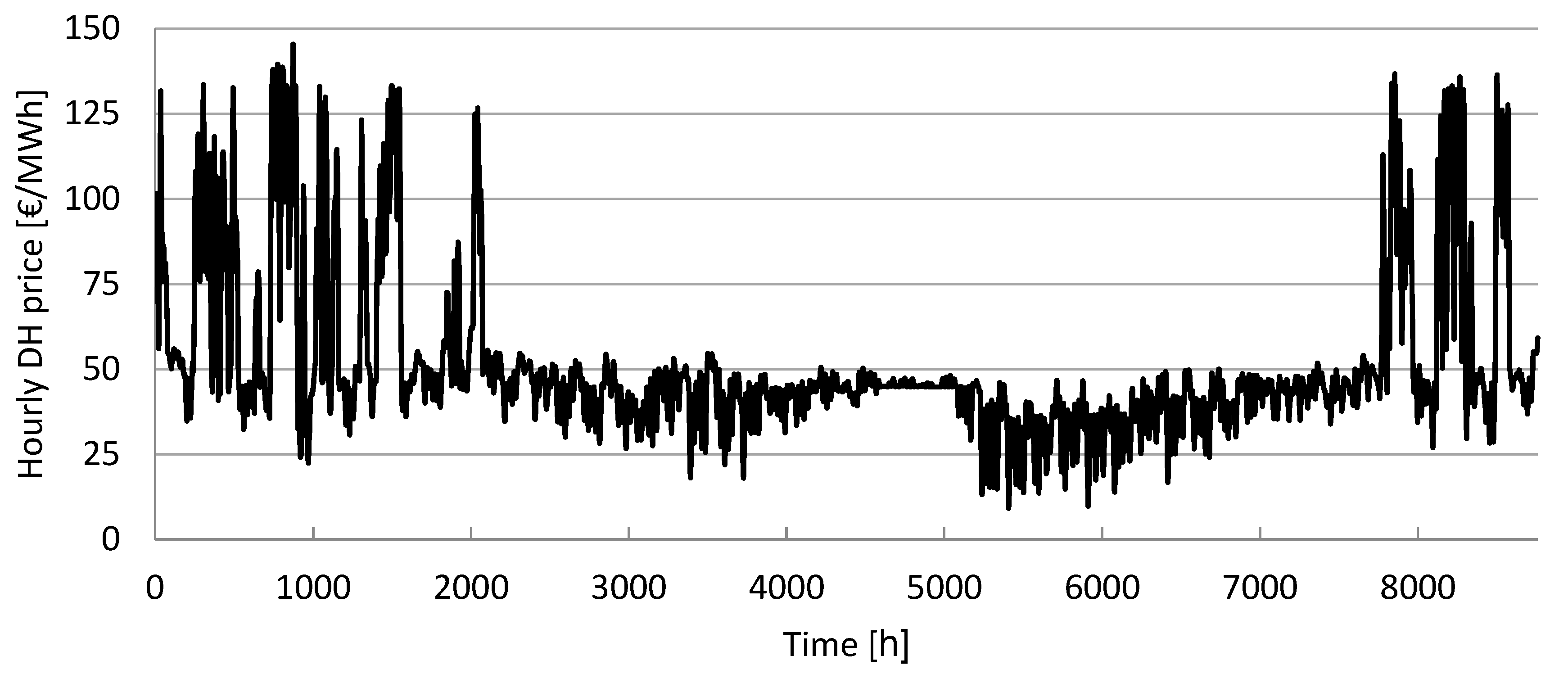
The prices remain stable during summer time (i.e., April to middle of November) with an average value of 40.5 €/MWh and a standard deviation of 7.7 €/MWh. During winter time, the corresponding values are 68.0 €/MWh and 29.7 €/MWh.
Figure 2 illustrates the hourly DH price used in the simulations.
It is assumed that all other buildings except residential and health care buildings can participate in DR actions. These count, for example, office, commercial and educational buildings which accounted for approximately 42% of the DH connected buildings in Finland in 2017 [
34]. The building types are anticipated to be similar in terms of water consumption profiles [
30] and weekly schedule (i.e., office hours). Therefore, it is assumed that the maximum share of buildings participating in DR is 42% in the DH network. It is further assumed that the heat demand profiles are similar in these buildings to receive an understanding of the potential of DR.
3. Results
3.1. Results from the Building Owner Perspective
Figure 3 shows the duration curve of specific DH power demand of space heating and ventilation of the cases presented in
Table 1 in
Section 2.1.
Figure 3 shows that the peak DH power demand of Case 3 is higher than the other cases for over 10% of the year, since the DR control charges, i.e., preheats the building by raising the set points of heating before high DH price periods. The analysis of Martin [
13] shows that the annual DH energy cost of Case 3 increases 0.4%, so it is not a financially viable case from the building owner’s point of view. The flexibility factor of heating based on the definition shown in [
5] is the highest of the selected cases (16.5%).
Furthermore,
Figure 3 illustrates that the DR control used in Case 2 slightly increases the peak power demand compared to the reference case. The peak power demand rises compared to the reference case because restoring the heating set points from the minimum level to the normal slightly increases the heating power demand. Case 2 achieves 5.7% annual heat energy cost savings, but its flexibility factor of 15% is slightly lower than in Case 3.
When cutting the peak power of the building by 35% (Case 4), the peak power demand for DH was below the reference case only 0.4% of the year. Correspondingly, the power was below the reference case from 3% (Case 5) to 8% (Case 6) of the year. From a building owner’s point of view, the cost saving potential of peak power limitation depends on how a DH distributor’s basic fee is compiled. If the contract power pricing is based directly on the nominal mass flow rate of the DH connection without additional charges, the annual power charge would decrease by 35% to 50% in the studied cases. However, the pricing system varies considerably across the industry.
3.2. Optimal Cases from the DH Operator Perspective
DR actions are expected to be profitable by providing cost savings and emission reductions in DH production. The effects of DR measures in DH production are summarized in
Table 3. The values were compared to the reference case, i.e., case without DR.
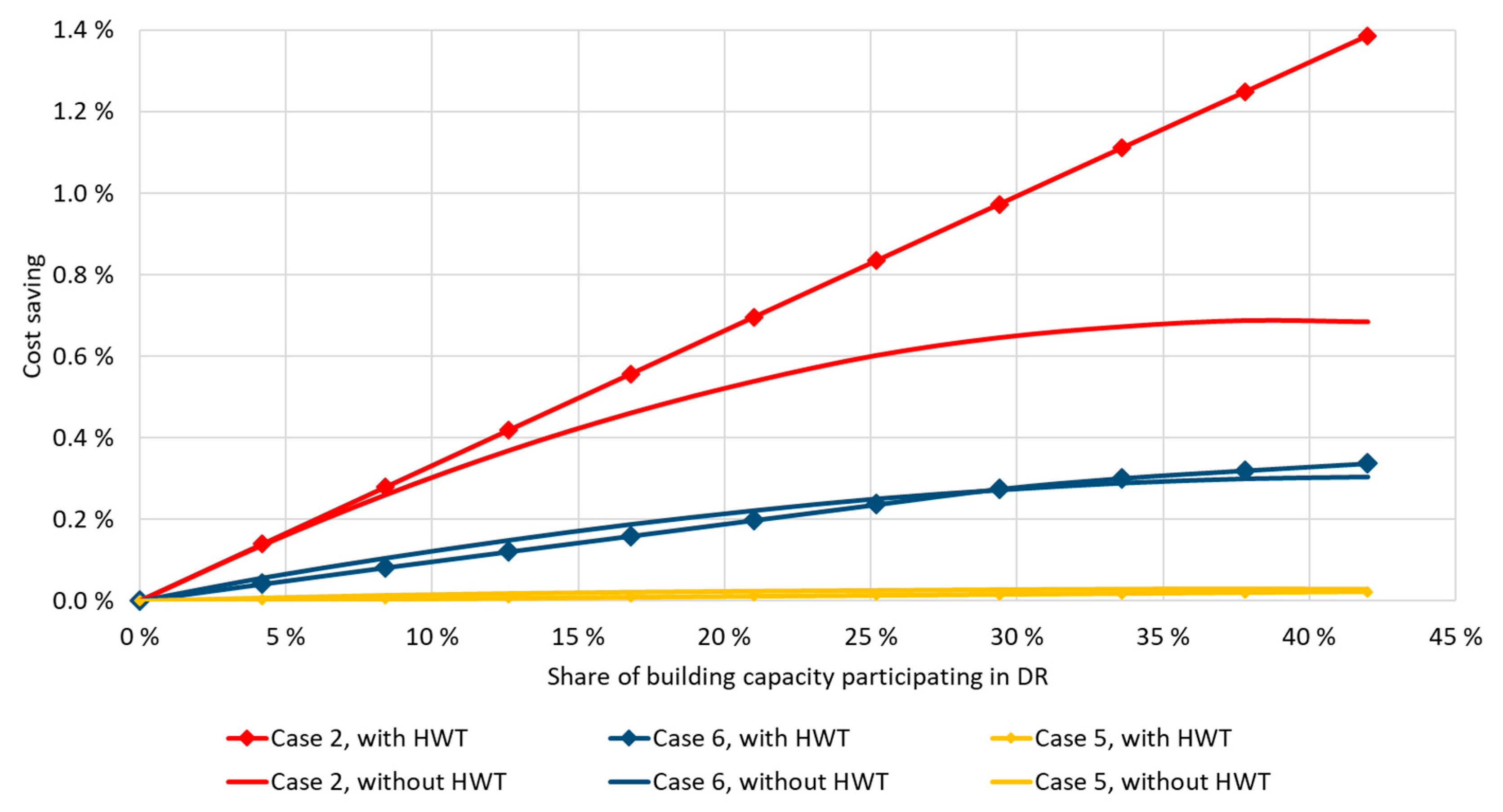
The cost savings as a function of building capacity participating in DR actions are illustrated in
Figure 4 and
Figure 5. The results are shown with and without an HWT in the DH system. The best three cases, i.e., cases 2, 5 and 6, are presented in
Figure 4 and the other two in
Figure 5. In the figures, the cost-saving potential is compared between DR-only strategy and DR with the HWT.
Yet, when HWT is included in the DH system, DR measures implemented in Case 2 decrease costs by 1.4% compared to the reference case. Furthermore, if HWT is not included in Case 2, the cost savings saturate when approximately 38% of the building stock participates. Increasing the share of buildings participating in DR can worsen the situation when HWT is not included, as seen in
Figure 4. This is probably because the sum of the heat loads shifted accumulate so that the HOB is ramped on, as cautioned in previous studies [
35].
The results indicate that Case 2 has the highest performance both in costs and emissions. These savings are, however, rather modest, at less than 1%, if HWT is not included in the DH system. The results thus suggest that it is worthwhile to combine HWT to DR actions. The optimal capacity of the HWT (i.e., the capacity after which heat production costs do not decrease even if heat storage capacity is increased further) is 20 GWh. This accounts for approximately 2% of the annual heat demand.
Case 2 was optimal from the building owner perspective as well. The DR algorithm only reduced loads during high-price times and hence was economic for the building owner. Consequently, the set point temperatures varied only between minimum and normal temperatures, and maximum temperature set points were not utilized.
Limiting peak power by 50% (Case 6) results also in slight cost reductions. However, too slight peak load reductions, i.e., −35% in Case 4 and even −43% in Case 5, do not affect the system costs. The buildings’ peak power demand does not always occur exactly at the same time when the system’s peak power takes place and hence Case 4 and Case 5 had an insignificant cost-saving impact.
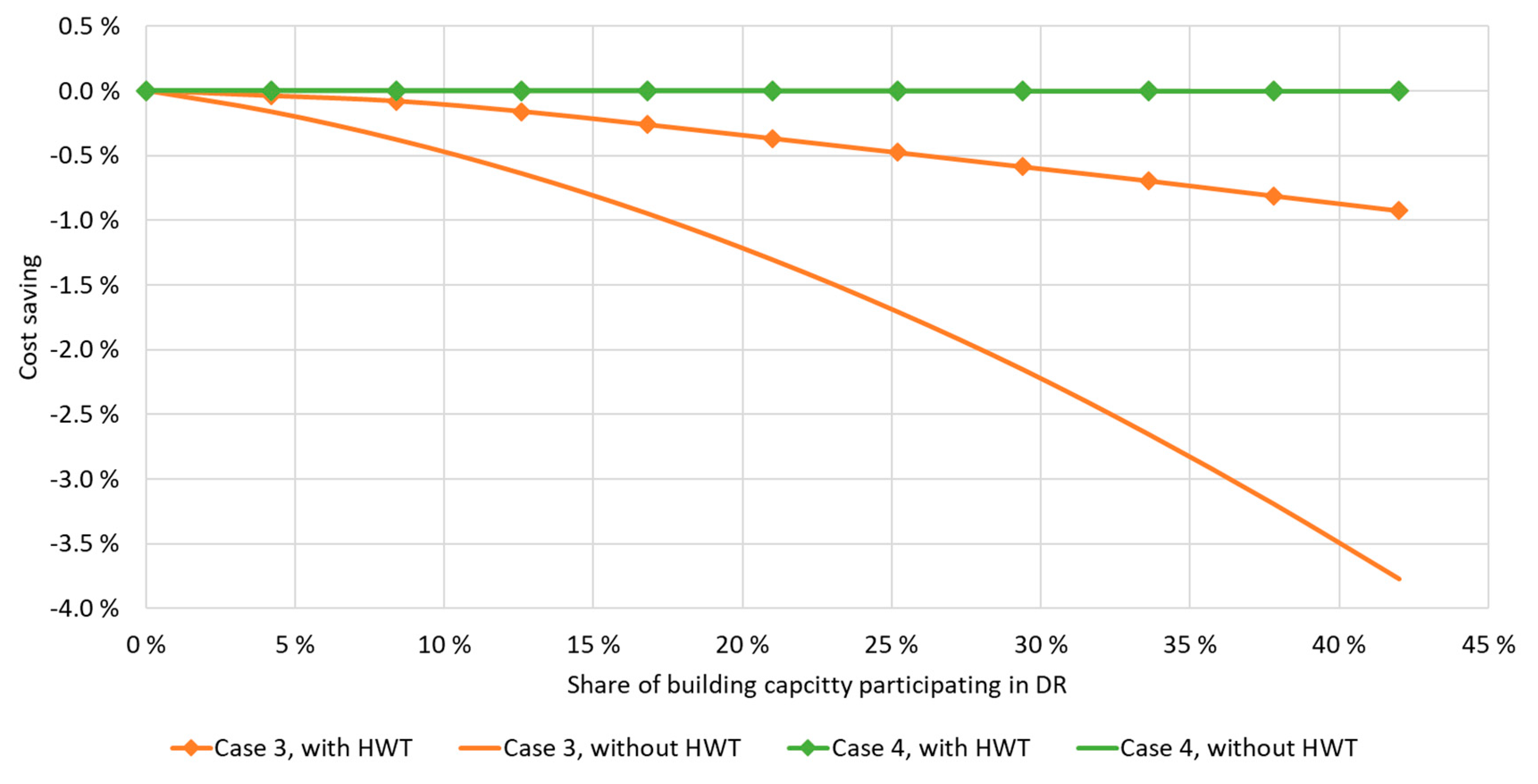
As seen in
Table 3, Case 3 does not have any optimal solution, i.e., by adapting the DR strategy used in Case 3, the costs will immediately increase. It is important to note that in some DR cases, i.e., Case 3 and Case 4, the heat production costs increase. This can be seen especially in Case 3 (
Figure 5) in which heat production costs increase almost by 4% if the whole 42% building capacity participates in DR. The strategy in Case 4 does not have any effect on the DH system. Case 3, however, can significantly increase costs compared to the reference case, as costs increase by 3.8% when implementing DR into 42% of the building stock. The HWT mitigates to some extent the short-term utilization of the HOB in Case 3 and thus diminishes slightly the cost curve.
As described in
Section 3.1, Case 3 was also for the building owner uneconomic as peak power increased significantly. Martin [
13] states that the simulated building does not benefit from heat loading probably because of the high ventilation air flow rate with its cooling impact on room air temperature, meaning that heat is not stored in the building structure.
The sensitivity analysis shows that when the whole building stock was controlled (= 100% DR participation), cost savings were 1.4% without HWT and 4.7% with HWT in Case 2. The emission reductions were approximately 2% both with and without the HWT in Case 2. Hence, DH operation optimization on building side and production side can be performed within these boundaries. Further results are exposed in
Table 4. As the cases were formed based on the simulation of an office and educational building, the strategies are unlikely to be optimal for residential buildings.
In the other cases, cost savings remained modest or turned even to slight cost increase. As can be anticipated already in
Figure 5, DH production costs increase significantly in some cases when connecting the whole building stock to the same DR strategy. Hence, charging all buildings at the initial low-cost hours affects counter wise for other peak load hours. The system has no iterative dynamic price signal which would prevent the formation of new peak prices, if enough building heat load has participated in a certain DR event.
If the energy reduction is not considered, and the system does not have the HWT, Case 2 is not beneficial when extracting DR actions to 42% of the building stock. The cost savings of Case 5 and Case 6 decreased slightly to 0.02% and 0.23% but remain advantageous. The HWT increases the profitability only a little bit. If the whole building stock is included and no energy saving is allowed, none of the cases are profitable.
3.3. Effect on Emissions
In the reference case, emissions of the heat and electricity production were approximately 0.36 MtCO
2, as the emissions from the CHP plant were 190 kgCO
2/MWh and HOB 284 kgCO
2/MWh. The emission coefficient for the CHP plant is calculated based on wood and peat consumption and the HOB based on oil consumption. Emission reductions cannot be reduced significantly with DR actions as illustrated in
Figure 6.
The highest emission reductions are gained with Case 2 and the decrease is less than 1% compared to the reference case. It can further be seen that the results with and without HWT do not significantly differ from each other. The amount of reduced emissions depends vastly on the DH production composition.
3.4. Fuel Consumption and Production Costs
Fuel consumption in the profitable DR cases is presented in
Figure 7. As can be seen, including the HWT in the system decreases the consumption of oil in the HOB. On the other hand, the HWT increases the consumption of wood and peat (i.e., fuels used in the CHP plant). The results thus indicate that with the usage of an HWT, heat can be produced more with the CHP plant, replacing HOB production. Adding DR has a trivial impact on fuel consumption.
As observed in
Figure 7, combining the HWT to DR actions appears beneficial. The inclusion of even a rather small HWT (5 GWh, i.e., 2% of the total yearly energy consumption) already decreases the generation costs by 18%. The annual costs of the system were approximately 15 MEUR. In Case 2, this means that costs were reduced by 0.2 MEUR in DR-only scenario and 3 MEUR with HWT. Although the HWT has significantly higher investment costs [
18] than DR technology, the HWT has an extensively shorter payback time. In Case 2, the investment in DR technology can cost a maximum of 1,447 EUR per building (á 3000 m
2; 150 kWh/m
2) for a 15-year payback time. This estimation includes only the cost savings for the DH company and does not consider the time value of money.
However, increasing the HWT capacity brings only marginal benefits.
Figure 8 presents heat production costs in the reference case and in the best performing DR cases (i.e., Cases 2, 5 and 6) as a function of the HWT capacity. It was also found that increasing the HWT capacity larger than 20 GWh does not affect production costs at all.
3.5. Impact on the Operation of the DH System
Key results of the operation of the DH system in the cases are presented in
Table 5. As can be seen, the CHP is operated non-stop when HWT is not used. Including DR measures do not change the HOB’s operating hours significantly (0.00–2.30% without HWT and 0.01–7.78% with HWT). The results in
Table 5 also indicate that using an HWT increase total ramp on and off costs, but it is anticipated that it reduces total cost savings only to some extent.
By comparing the reference cases, both with and without HWT, the production capacity of the HOB is reduced to approximately one third when adding the HWT to the system. The results indicate also that without the HWT in the system, the operating hours of the CHP unit are the same in each DR case. When the storage is included, the CHP plant is always run in cogeneration mode. The number of operating hours as well as heat production with the CHP plant are lowest in Case 2. HWT increases the number of start-ups and the heat production with the CHP plant. The HWT also decreases heat production with the HOB considerably. It can be further seen that when the HWT is included in the system, DR actions reduce heat production with the HOB compared to the reference case. The results thus suggest that including an HWT in the system efficiently transfers production from peak load to base load. Consequently, this can also mitigate the temporary overproduction from the DR strategies and hence increase the benefits of the DR actions.
In Case 2, heat production with the HOB is a bit higher than in the reference case or in the other profitable DR cases when HWT is not included in the system. On the other hand, heat production with the CHP unit decreases by 9 GWh. That amount compensates the usage of oil-fired HOB and the decrease in electricity revenue (
Figure 9).
As shown in
Table 5, the number of HOB start-ups decrease significantly when implementing the HWT to the cases. The number of CHP start-ups does not significantly change even though the start-up costs are doubled [
18]. Revenues from electricity sales drop slightly or remain the same in purely DR cases. When adding the HTW to the system, revenues grow by 11%. However, adding an optimal DR scheme to the system changed revenues less than 1%.
The relative hourly variations are calculated based on [
4].
Figure 10 presents a part of the duration curve of the DH system’s relative hourly variation. The load variation grows significantly in Case 2 as the algorithm only reduced loads during high-price hours. The higher variations show that the heating set point temperatures vary between minimum and normal values. The difference in electricity revenues between Case 5 and Case 6 compared to the reference case is very small as those cases focused on cutting annual peak load, which is usually set during winter months. The other cases are not presented because of their uneconomic results in
Section 3.2.
Compared to the research by Romanchenko et al. [
19], in which heat load variations decreased by approximately 20%, the load variation growth in Case 2 is significant. The results indicate that an increase in load variation does not necessarily mean an increase in DH production costs. However, this depends extensively on the selected power plants. The relative hourly variation curve for the whole year is provided in
Appendix A Figure A1.
The heat load curve of the reference case is presented in
Appendix A Figure A2. Case 2 is drawn in
Appendix A Figure A3. It can be noted that the heat load curve is generally affected during mid-season, i.e., spring and autumn time, as stated in previous research [
8], [
12]. During the coldest winter days, the load cannot be decreased for longer time periods, as high heat losses affect room-air temperature and thus building users become dissatisfied, as recognized, for example, in Case 6 in
Section 3.1. On the other hand, temporarily increasing the load during winter-time is challenging as the system is on its limits already, and energy is squandered in heat transfer through the building elements, as described in Case 3 in
Section 3.1. During summer-time, DR has not been performed and hence the load curve is not affected. HWT, on the other hand, is beneficiary to utilize during summer-time, as described in the following section.
3.6. Heat Storage
Figure 11 illustrates how the heat store content changes in the DR cases 2,5 and 6 compared to the reference case. As can be seen, the HWT is charged almost to its full capacity during June and mid-July and it is discharged until early August.
The seasonal variations of thermal store content do not differ between the cases. Only minor daily and hourly variations are observed. As summer-time heat demand consists almost only of DHW, the thermal store content of each HTW case does not differ from the reference case. Despite the fact that the HWT charging and discharging rates (i.e., heating power) cannot be controlled in energyPRO, the rates remained within acceptable ranges.
4. Discussion
Sameti et al. [
36] distinguishes challenges in modelling and optimizing district-level systems: it includes spatial aspects connected to the location and temporal aspect associated with consumption, production and price profiles. Similar boundaries can be distinguished in this research: the profitability of DR varies with the network and power plant composition. However, previous studies have indicated also low-cost savings and uncertainties with reimbursement [
8,
19]. Even though load profiles can be shaped extensively on the building level, these opportunities have not been found profitable for the DH producer. As the prospect of DR seems logical, further research should be performed on merging demand-side control strategies with production-side realities.
As DR has been investigated in this study as a signal given by the DH operator, but fulfilled by the demand side, the operator has only partial control of the load steering. On the other hand, utilizing an HWT enables the DH operator to completely control the load within the maximum capacity. Also, the DH network with its mass of circulating water itself has been taken only simplified into account in the simulation. The network’s ability as a TES has been recognized [
37], but its buffering capacity of the DH network is limited [
38]. This means that heat load variations can be still significant even after the pipe network is used at maximum capacity.
The Finnish DH industry has been skeptical about the profitability of DR. Based on DH companies’ assessments, the realistic estimate for the total commercial benefits of DR are 1–3% of annual costs based on current solutions and current experiences [
35]. Also, former research received similar results with less than 2% cost reduction [
8,
20]. Although there could be a benefit for the building owner, the DH operator requires accurate opportunities on DR before deployment. The demand for DR implementations may rise in the near future, as in [
20] it is argued that in 2029 the benefits of using short-term TES is greater through the increased amount of intermitted generation that can be integrated into the DH system.
The assumptions for the DR cases are based on dynamic hourly prices for DH, which is not state-of-the-art in current systems. Furthermore, the DR strategy needs a dynamic pricing system in which the predicted load profile is iterated with each participating building, forming a new price and hence giving an incentive for further buildings to participate in demand shaping at the right hour. This iterative process can diminish the shifting of load to another high-cost production hour. The accumulation has been distinguished as one of the most important factors why DR alone did not bring savings to the production side in this research.
5. Conclusions
The effect of different DR strategies has been simulated in a typical Finnish DH system. The installed thermal power accounted for 396–504 MW
th and electrical power for 108 MW
el through the biomass-fired CHP plant. The oil-fired HOB had a heat output of 200 MW
th. The cases have been simulated also with an HWT (i.e., large thermal water storage). The DR strategies focused on commercial buildings (i.e., office premises, schools and public buildings). This accounts for 42% of the total building stock in the simulated system. The selected cases have been retrieved from previous research in which the building’s thermal inertia has been profoundly studied in a Finnish environment [
13].
The results of this study are in line with previous research: DR has only a slight positive effect on costs and emission levels in a DH system. While a DR-only strategy results in rather modest savings, adding an HWT can enhance the optimal control strategy. The best investigated DR control strategy was Case 2, where DR was performed in space heating and ventilation when the price trend was declining. If the HWT was included, costs decreased by 1.4% and emissions decreased by 0.8% when 42% of the building stock participated in DR. Case 2 was optimal also for the building owner when considering dynamic DH prices.
Furthermore, the HWT can diminish harmful DR strategies, as seen in Case 3 (i.e., performing DR in space heating and ventilation when the price trend was either rising or declining). This case was also uneconomic for the building owner. Overall, investing in an HWT alone can bring benefits, including DH cost reductions of 18% and an 11% rise in electricity revenue. However, this does not consider the large capital investment. The sensitivity analysis, in which the cases were scaled to the whole building stock, showed that further cost savings were achieved in Case 2. However, charging all buildings with the same strategy at the initial low-cost hours can lead to the formation of new peak load hours. The cost-saving potential depends on the time of DR and amount of buildings participating in the same strategy.
From this paper, the following recommendations can be made: first, the right DR strategy is crucial for the production-side perspective. With a dynamic price for DH, the building owner can perform multiple DR actions which would be beneficial for him but not necessarily for the energy company. Hence, it is important for the energy company to plan actions beforehand and grant the right incentives to the market. Second, the composition of the DH network and the thermal plants can affect DR operation considerably and, therefore, savings in production costs and emissions. Third, adding an HWT to the DR cases enhances the CHP and HOB operations and thus decreases costs. Utilizing HWTs is not overlapping with DR control, but rather enables a larger share of the building stock to participate in DR as overproduction can be compensated.

 ,
, 


