1. Introduction
In recent decades, induction motor (IM) applications have been extended to various fields in industry due to their numerous advantages, such as low cost, less maintenance, simple and robust construction, high efficiency with good reliability in operation than any other motors available. If a fault occurs in an IM and is not identified at the earlier stage, it may lead to unplanned downtime and economical loss to the industry, and even sometimes results in catastrophic effects to the industry [
1,
2]. Thus, some industries have started performing maintenance to safeguard the equipment by detecting the faults at the earliest. On the other hand, maintenance may lead to a production blockage in the industry by consuming more time for diagnosis. Many studies [
3,
4] keep on suggesting the importance of condition monitoring (CM) and fault diagnosis of IM, which is more recommended to avoid the production blockage for diagnosing the IM. Generally, CM deals with continuous monitoring of the failure progress of respective equipment, and indicates the significant changes observed above the critical level. The CM in IM can be done by monitoring any of its own parameters, like voltage, current, magnetic flux, etc. The online surveillance of IM progressively cuts down the scheduled maintenance cost and automatically increases the production rate by reducing the diagnosis time.
According to IEEE survey [
5], bearing failure (44%) is most frequent in IM rather than any other faults, and thus research based on bearing has been taken for the present study. Frequently observed bearing faults are pitting, scratch, flaking of the surface, and abrasion [
6]. These faults are mainly due to misalignment, environmental condition, mishandling, voltage fluctuation, contamination, corrosion, insufficient lubrication, overloading, and bearing current [
7]. If a defective motor continues to operate, it may exhibit symptoms, like temperature rise, vibration, changes in the harmonic components of current, and variations observed in the electromagnetic field, which gradually reduce its function and result in motor failure [
8].
Among the various diagnostic methods, vibration analysis [
9,
10], motor current signature analysis (MCSA) [
11], acoustic emission (AE) [
12], and stray flux monitoring [
13] are widely practiced. The vibration analysis is a traditional method, but parameters like cost, access, and placement of vibration sensors make it difficult to gain use in practical cases. In the case of MCSA, being a non-invasive technique, it avoids the disadvantage of the vibration method by eliminating direct access and sensor requirements but, again, fails in determining the present state of the bearing condition. Additionally, AE and stray flux methods need to have direct access to the motor. Many studies are attempting to find the ideal and effective technique for diagnosing bearing failure. In addition, non-invasive techniques are preferred because of easy access and low cost. Therefore, it is necessary to develop an effective CM with a non-invasive technique for early identification of the fault.
In recent decades, the application of digital signal processing to detect bearing faults in IMs has been extended [
14]. It produces reliable output by interpreting the statistical data. Generally, raw signals collected from the experiment are not enough in identifying the fault [
15], therefore, fault features need to be extracted from any of the three methods: time domain [
16], frequency domain [
17], or time-frequency domain analysis [
18]. Many studies have performed bearing failure analysis considering a hole [
19] as a faulty factor. On the other hand, scratches in the bearing have a high probability of occurring and should be considered for performing bearing failure analysis. The fault should be detected at the early stage, which is during the minor stage, so that sudden breakdown in industries may be reduced. Thus, studies based on scratch and minor fault detection need greater attention.
Bearing fault diagnosis relies on ML and AI to have a better CM system and, thus, it may increase the reliability of the motor. Generally, ML has been used in telecommunication, medical diagnosis, market analysis, weather prediction, image sensing, etc., where its application gets globalized. In ML, a wide variety of algorithms are available and, based on the application, the algorithms are selected. The different styles of ML algorithms are supervised, unsupervised, and semi-supervised. Supervised learning is about inputting the known data and evaluation is performed based on the probability. In contrast, in unsupervised learning the input data are not known, and the algorithm is designed to detect the structures of the data. In the case of semi-supervised learning, input data are a mixture of labeled and unlabeled values as an input function and the evaluation is performed. The application of ML for the purpose of diagnosis and prediction in other fields are studied [
20,
21,
22]. Additionally, AI has been a growing technology in all fields which are competitive to ML algorithms. In recent days, the application of AI to fault detection has increased; artificial neural network (ANN) and adaptive neuro-fuzzy inference systems (ANFIS) [
23] are mostly investigated. The application of ML and AI is a challenging task, but if the outcome of the approach satisfies the industrial requirement, then data processing through ML and AI will be the best choice in the fault detection of IM.
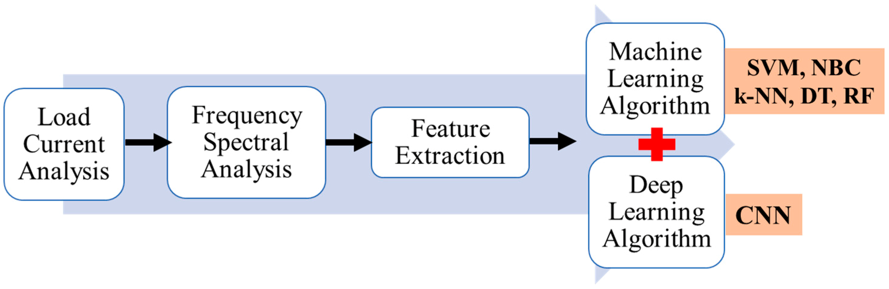
The present work aims to develop a non-invasive and inexpensive diagnostic tool for detecting a minor bearing fault in an IM at the early stage by using the various ML approaches and AI. Among the ML, support vector machine (SVM), naive Bayes classifier (NBC) algorithm, k-nearest neighbor (k-NN) algorithm, decision tree (DT), and random forest (RF) are selected. In AI, deep learning (DL) with a convolutional neural network (CNN) architecture is selected and discussed. For making the proposed system to be accepted by industry, the rotating speed is not taken into account in the proposed diagnosis method. The scratch and hole are considered as the faulty factors. Initially, an experiment is conducted at different load conditions and the frequency spectrum of the load current is obtained by fast Fourier transform (FFT) analysis. The features are extracted and used to train the ML and DL algorithms. Finally, the difference between the ML and DL are evaluated and its application towards motor fault detection is discussed. The concept of the method proposed is illustrated in
Figure 1.
2. Experimental Setup and Fault Specification
A specimen of the present study is a three-phase IM (2.2 kW, 200 V, 8.5 A, 1740 min
−1, four poles).
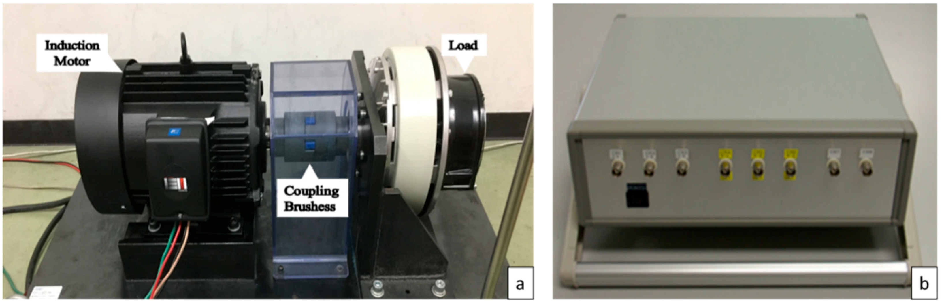
Figure 2a shows the experimental setup and a powder brake is connected to the IM as a load. The rotating speed of the induction motor can be varied between 1780 min
−1 and 1765 min
−1 by changing the load parameters. The current sensors (HIOKI, Type 9696-02), voltage sensors (HIOKI, Type 9666), and a tachometer (ONOSOKKI, Type HT-5500) continuously monitor the load current, line-to-line voltage, and rotating speed, respectively. The developed instrument with seven A/D converters is effectively used to transfer data from these sensors to a desktop computer and shown in
Figure 2b. Frequency resolution of the instrument is about 0.76 Hz because the sampling time is designed to be 10 μs, and the data recording length per channel is 2
17. Data transfer is performed in less than 20 s and the data acquisition command for every 30 s. The power supply frequency is 60 Hz.
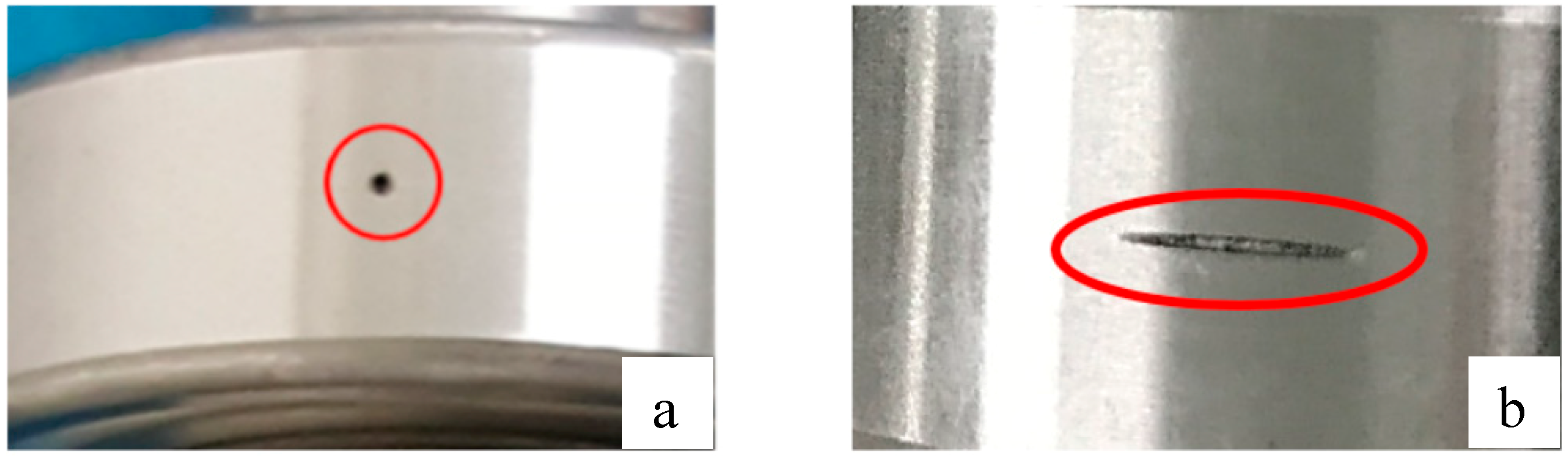
The collection of bearings with defects from the factories is arduous and consumes time. Alternately, an artificial fault is induced on the outer raceway of the bearing and the diagnosis is performed. Initially, healthy bearing data are taken for reference and the next experiment is carried out after replacing the healthy bearing with a faulty one. The bearing conditions used in the present study are shown in
Figure 3. The fault specification details are: the diameter and the depth of a hole are 0.5 mm and 0.5 mm, respectively. A scratch has a size 5 mm in length and 0.5 mm in width and depth. The bearing conditions are indicated as follows: H, healthy; F1, failure with a hole; and F2, failure with a scratch.
5. Diagnosis Using Machine Learning (ML)
Generally, ML algorithms are classified as supervised and unsupervised algorithms. The supervised algorithms consist of target variables which are to be predicted from a given set of independent variables. These variables are used to generate the function and maps of the input to obtain the desired output and to achieve the objective. The data are trained to achieve a better accuracy rate. The training process is continued until the model achieves the desired level of accuracy. However, in the case of unsupervised algorithms, there is no target variable and the clustering technique is adopted. The techniques may segment the group and certain levels of diagnosis can be achieved. The role is to identify the current condition of the bearing and from the case study it is known that the supervised machine learning algorithm is suited. The algorithms used in the present study are SVM, NBC, k-NN, DT, and RF, and python is used as a diagnostic tool.
5.1. Support Vector Machine (SVM)
SVM [
24] is a well-known pattern recognition algorithm mainly used for classification and regression problems. The basic parameters of SVM are the hyperplane and margin. The hyperplane separates the datasets and performs the classification task and the margin identifies the support vectors of the datasets. SVM performs classification by finding the optimum hyperplane that maximizes the margin width between the classes. The high margin width avoids the overlapping issues between the classes. Generally, the margin is classified into two types: soft and hard margins. Since the present diagnosis deals with the non-linear classification problem, a soft margin is used.
The accuracy of the SVM will be affected by three factors: the threshold function, the cost parameter (C), and the kernel function. Recognition ability can be improved by the threshold function. The cost parameter adjusts the tradeoff between the smooth decision of the boundary condition and classifying the training points. Low bias and high variance can be achieved when a large value is used as the cost parameter. The main role of kernel functions is to map the input at high dimensional features so that non-linear classification is available. Radial basis function (RBF) has been selected in the present study. In RBF kernel, data classification is affected by gamma parameter. The gamma parameter sets the pattern contrast to the cost parameter. The values of the cost and gamma parameters should not be very high because of overfitting, and they should not be very small because of underfitting problems. These parameters can be tuned through programming by selecting the optimum ranges.
The selection of optimal hyperplane is mainly based on the training features. Techniques, such as cross-validation, re-sampling, and grid search, help in selecting the values of the cost and gamma parameters automatically during the diagnosis. Cross-validation in ML helps to train the model using optimal hyper-parameters. Re-sampling is a series of methods used to reconstruct the sample data sets, including training and testing datasets. A grid search is an iterative method of choosing the best parameter value for an ML model. The optimized values of C and γ with the highest accuracy rate are used in the present study and the corresponding hyperplane is constructed. Specifications of the SVM used in the present study are described in [
25] and explained in
Table 1.
5.2. Naive Bayes Classifier (NBC) Algorithm
The probability of occurrence of an event can be analyzed by the NBC theorem [
26] using evidence or data. The conditional probability and the assumption of attributes are independent of each other and should be considered in the NBC theorem. In spite of its simplicity, NBC enables quick and effective analysis by using high dimensional datasets. NBC is suitable to the case where large supervised or unsupervised data are processed and the classification is performed in a limited time. In the present study, a naive Gaussian is selected because it matches our prescribed condition.
In the present study, a NBC algorithm is created considering the basis of conditional independence P (X|Y), where X = (X1, X2, …, Xn) which is used to specify the number of parameters in training and Y is used to emphasis the selected condition of X. The value of each subset P (X|Y) is calculated according to the input X and the problem of estimating the training data is neglected.
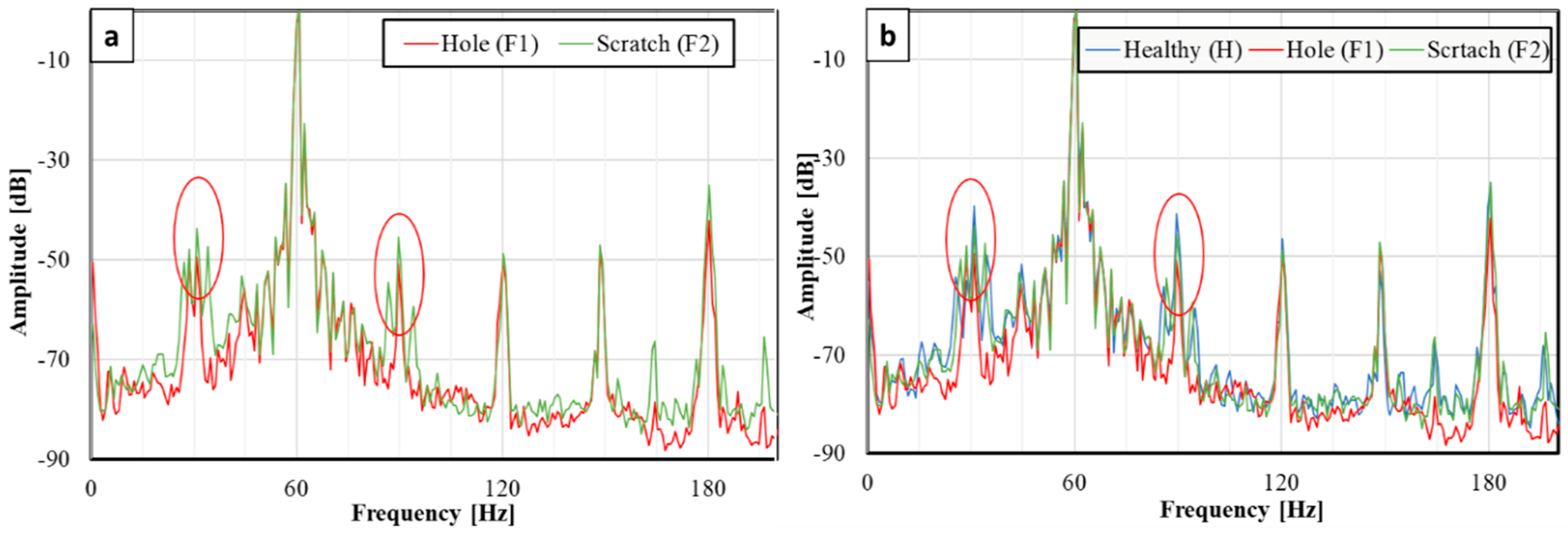
In the current study, X is 3 (the number of the bearing condition) and Y is 2 (amplitude of 30 and 90 Hz components). To map the input data in a three-dimensional network, a kernel function is used. Training of the algorithm is performed to obtain a high accuracy rate by importing the data selected randomly.
5.3. K-Nearest Neighbor Algorithm (k-NN)
k-NN [
27] is non-parametric and versatile learning algorithm used for both classification and regression problems. Generally, this algorithm memorizes the training datasets instead of learning the discriminative function. The instance-based learning helps in avoiding errors by memorizing the training sets. In the model, the non-parametric is not fixed in advance and it varies based on the data size. The disadvantages of k-NN is its large memory storage, long prediction time, and unnecessary sensitivity to irrelevant features.
k-NN performs classification on testing data based on the k-nearest training samples around the test data. Mainly k-NN depends on two things: (1) a distance metric which is used to compute the distance between two points; and (2) the value of “k” which is used to define the number of neighbors. The value of k decides the shape of the decision boundary. The boundary becomes smoother if the neighbor selection increases the value of k. Technically, small k values result in a hard boundary condition, but it still gives a more flexible fit with low bias and high variance.
In the present study, the value of k is selected in the range of 1–50. With this condition, the boundary becomes smoother and the boundary condition becomes adoptable to any classes of condition. The main objective to get the maximum accuracy rate with high variance condition. Thus, the low bias condition is made possible, making the method suitable to identify the present condition of the bearings.
5.4. Decision Tree Algorithm (DT)
A DT [
28] is a dendritic classification model used for both classification and regression problems. The classification is performed by the breakdown of data into smaller subsets and mainly based on the feature selection. The final structure is like a tree with branches and leaf nodes. Each node represents a feature (attribute), each branch represents a decision (rule), and each leaf represents an outcome (categorical or continuous value). A given set of data is divided into several sets, stepwise. The models are recursively constructed from the root node and every possible outcome of the condition is analyzed. If a condition passes through at one root junction, the decision is made at that moment and the output is displayed. If the condition becomes false, it moves to the next stated condition and the process gets repeated until the output is decided.
The constructed DT reaches tis optional depth depending on parameter n. Additionally, it is important how many times these branches containing the parameter-n is used as root junction to the analysis. If n is too small, the accuracy may be low. However, when the optimization is performed for larger values of n, the count of missing data is increased. Thus, considering the condition, the value of n is selected as 5 in the present study.
5.5. Random Forest (RF)
The RT [
29] is a classification method where the output is decided by the majority rule using the results of plural DTs. First, a DT is constructed by random data extracted from the training data. Then the technique named tree bagging is performed n number of times. Each DT is branched by an explanatory selected variable which has the highest purity. More DTs are constructed, and the class function is established. The output is concerned with majority of the voting and the final class is declared. Thus, the RF has a better output when compared to the DT algorithm but takes more time for commutation. The class division and the selecting/deciding the result of the majority voting is performed by the bagging function, which is nothing but the tree bagging. For the point of reliability, the value of n is chosen in such a way that an acceptable accuracy rate should be obtained, and the count of missing data should be less.
In the present study, three classes of DTs are selected and framed to form the RF. The DT takes the n value 4 and the bagging technique is performed. Between the three classes of DTs, selection of the variable is done randomly, and the major voting is performed using the tree bagging function to carry out the diagnosis.
5.6. Diagnosis Procedure
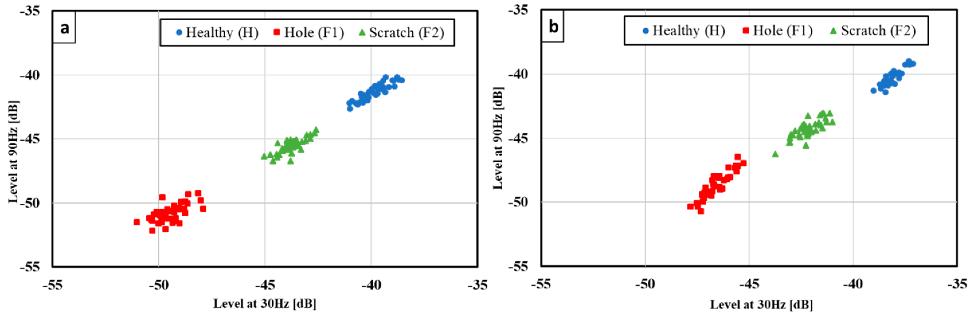
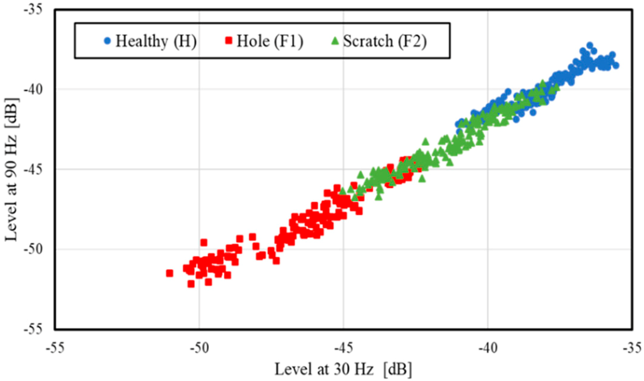
Using features, i.e., amplitudes of 30 and 90 Hz components, shown in
Figure 6, diagnosis is performed. Features are divided into two categories randomly in the ratio of 70:30. Seventy percent of features are used for training the algorithm and the remaining 30% for evaluation. The same procedure is repeated for all the algorithms described above. The entire diagnosis is carried out in python for all ML algorithms. Based on the evaluation, the accuracy rate of each algorithm is obtained using the formula defined in the programming in python, i.e., the accuracy rate in the present paper is given by:
5.7. Diagnosis Result
To distinguish the faulty bearing from the healthy one, diagnosis for the bearing condition of healthy (H) and hole (F1), and healthy (H) and scratch (F2) is performed. Diagnosis of conditions F1 and F2 is also carried out to discuss the possibility of fault identification. The rotating speed is not considered for any diagnosis. In case of HF1 combination, a total of 320 data points are selected, where 240 data points are used for training and 80 data points are used for evaluation. In the same manner, data selection is done for other bearing combinations (HF2 and F1F2).
Table 2 shows the accuracy rate of the diagnosis using various ML algorithms.
Each ML algorithm stands unique in its characteristics and were found to be more effective in detecting the bearing faults accurately. A 100% accuracy rate is obtained between HF1 bearing conditions in all the algorithms. In the case of HF2 bearing conditions, the k-NN algorithm acquires a higher diagnosis rate than any other ML algorithms. The DT algorithm produces a low accuracy rate of 78.75%. SVM, being a powerful algorithm, produces an accuracy rate of 81.96%. The other algorithms, k-NN, NBC, and RF, produce diagnosis rates of more than 80%. The average diagnosis rate of each algorithm is high in the case of diagnosing minor faults in bearings and to be accepted practically. In the case of diagnosing F1F2, all the algorithms produced high diagnosis rates of more than 90%. Thus, no further study is required in the case of F1F2 bearing conditions.
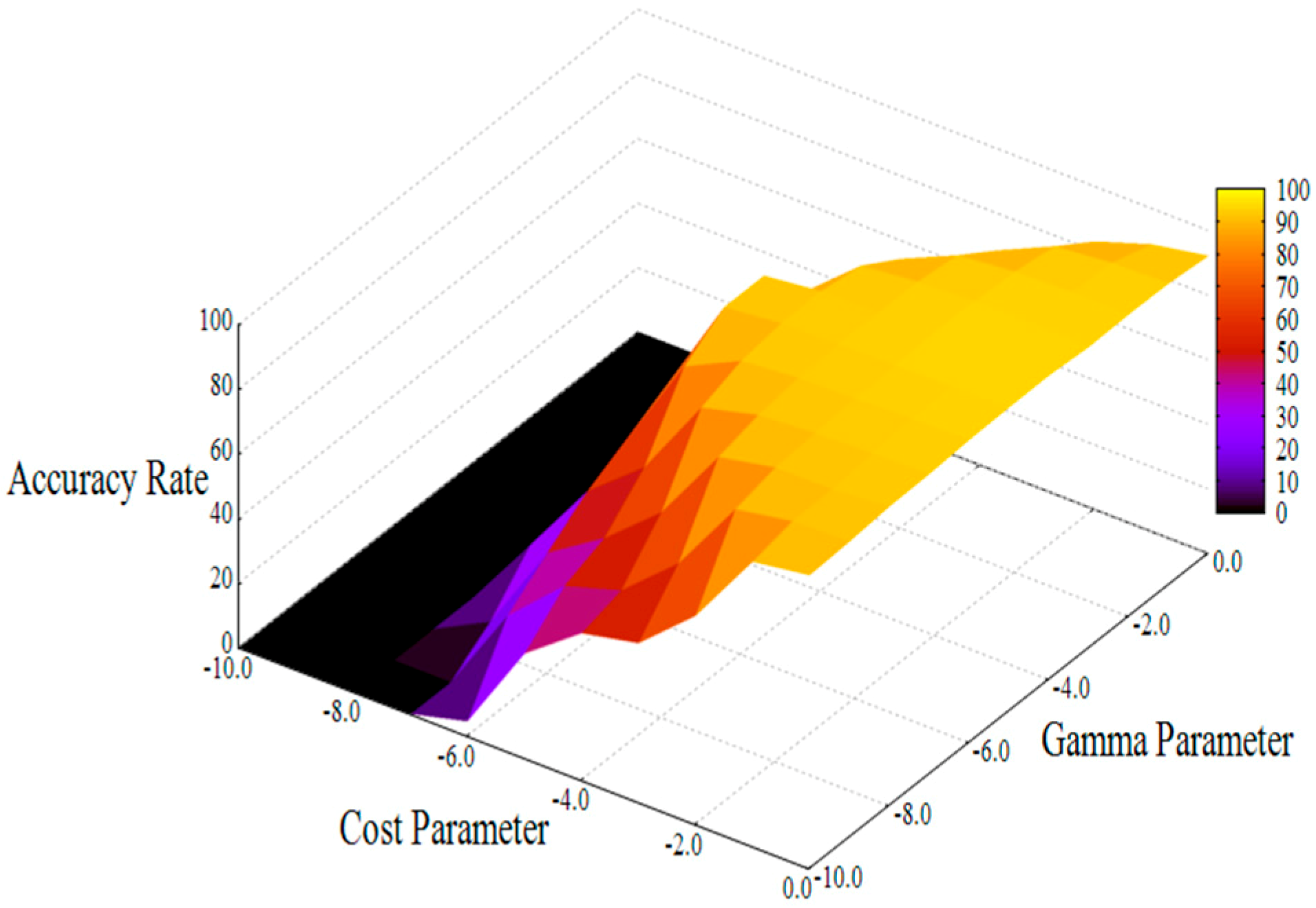
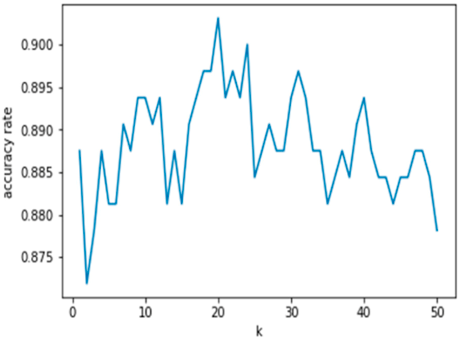
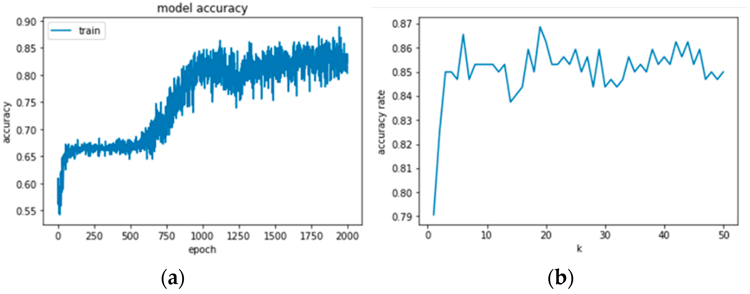
The diagnosis accuracy results in the case of F1F2 for SVM and k-NN are shown in
Figure 7 and
Figure 8, respectively. The result of SVM (
Figure 7) shows the variation of accuracy rate with respect to the cost and gamma parameter. The optimization of parameters is performed, and the highest accuracy rate is obtained.
Figure 8 represents the k-NN diagnosis result. The value of k selected between 1 and 50 is indicated and the maximum accuracy rate is achieved with a k value 20. Both the SVM and k-NN show acceptable diagnosis rates.
While using ML, not only should the accuracy rate, but also the missing data calculation, be considered. NBC, DT, and RF are probability-based algorithms. In that case, the amount of missing data is said to be high and the reliability of the acquired result shall be low. On the other hand, both the SVM and k-NN are independent of the probability and the algorithm truly depends on the tuning parameter like the cost and gamma parameters, the threshold function, and k value. The accuracy rate depends on how the tuning is performed and how the hyperplane is constructed. The amount of missing data are low and the reliability and versatility of the algorithm is said to be high. Thus, among the various ML algorithms, k-NN and SVM take priority and can be employed in diagnosing the motor failure in the industrial environment.
7. Conclusions
In this paper, a detailed study about the application of ML algorithms and the DL to machine failure diagnosis is carried out. The hole or scratch is selected as a fault for the analysis and the diagnosis is performed without taking the rotating speed in to account.
The diagnosis results of all ML algorithms belong to the same range, yet SVM and k-NN have higher accuracy rates. From the study, the diagnosis method can be selected according to the application. For example, if a large number of bearing conditions is discussed, k-NN and SVM are the preferred algorithm. If the number of bearing conditions is less, for example two or three classes, it is better to go with RF, DT, or NBC. These RF, DT, or NBC algorithms become complex in the case of multiple classes; this is because of the probability-based procedure, as it takes more time for commutation and produces a lower accuracy rate and low reliability.
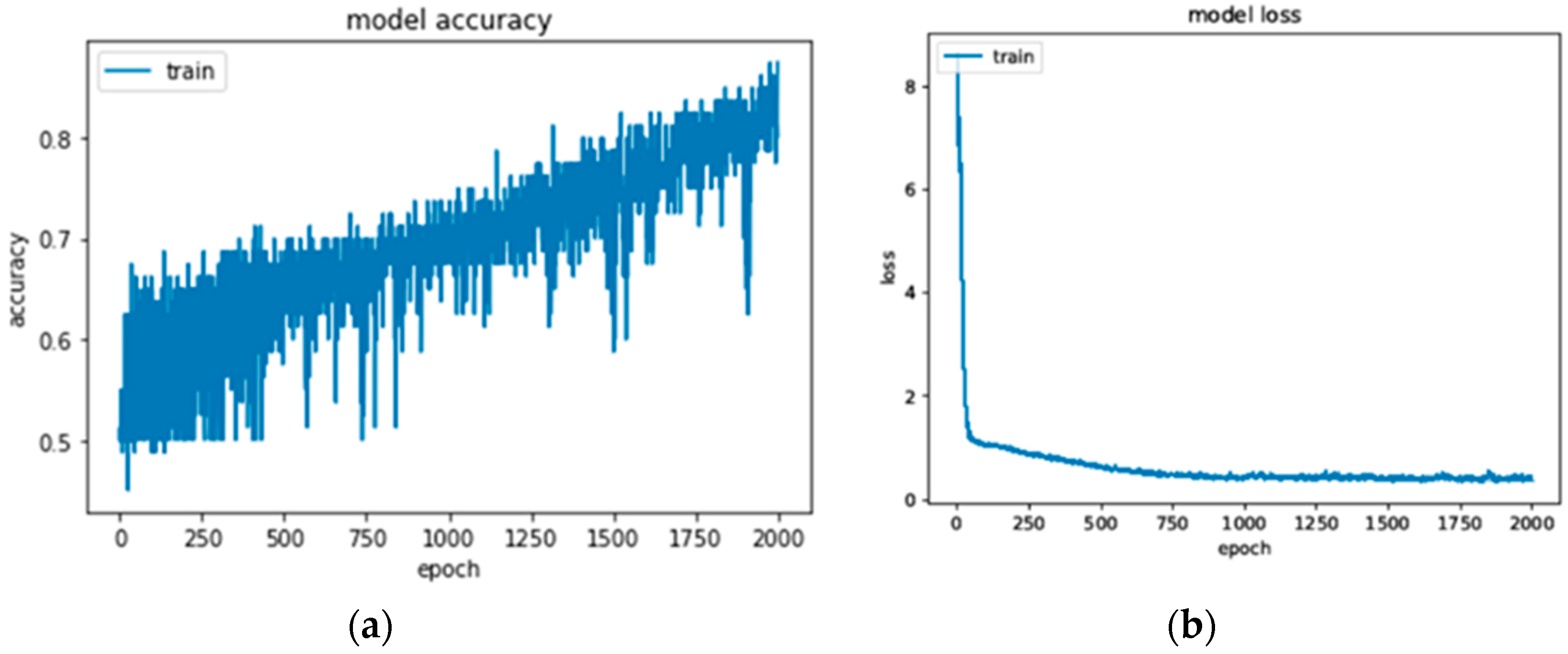
Finally, a trail to bring the DL algorithm to motor fault diagnosis is achieved and the results are promising and acceptable. It has many advantages over ML algorithms, as it can be trained for any kind of application. The time consumption is less, and programming skill is not required to tune the parameters. The only disadvantage of the CNN is the requirement of the large data count to achieve diagnosis with high accuracy.


