Investigation of Laminar–Turbulent Transition on a Rotating Wind-Turbine Blade of Multimegawatt Class with Thermography and Microphone Array

 , , , and
Abstract
1. Introduction
2. Experiment Setup
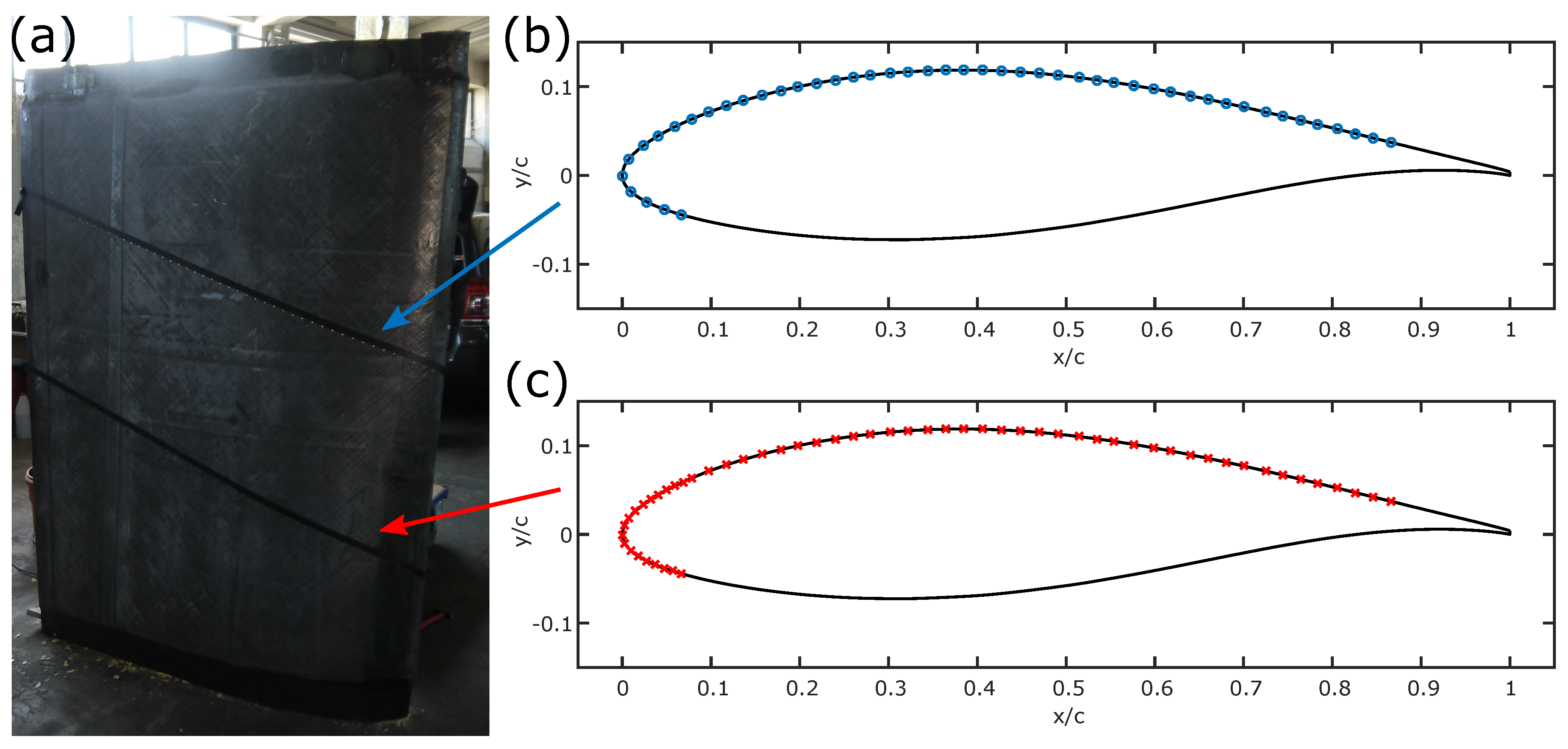
2.1. Aerodynamic Glove
2.1.1. Turbine and Site
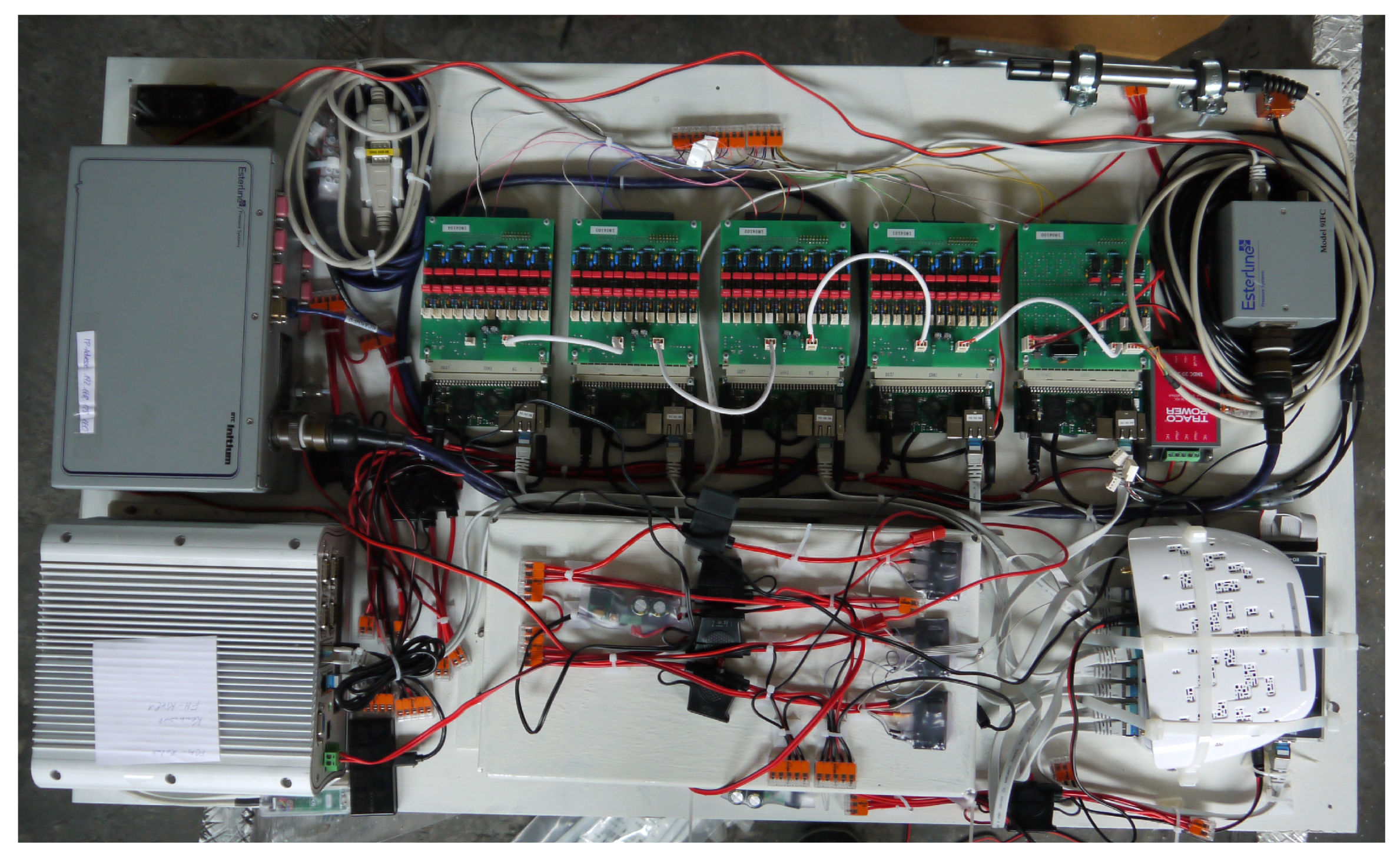
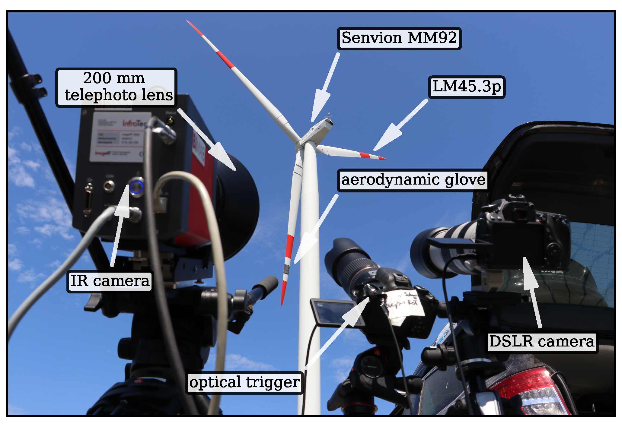
2.1.2. Overview of Experiment Setup
2.1.3. Aerodynamic Glove
2.2. Thermography
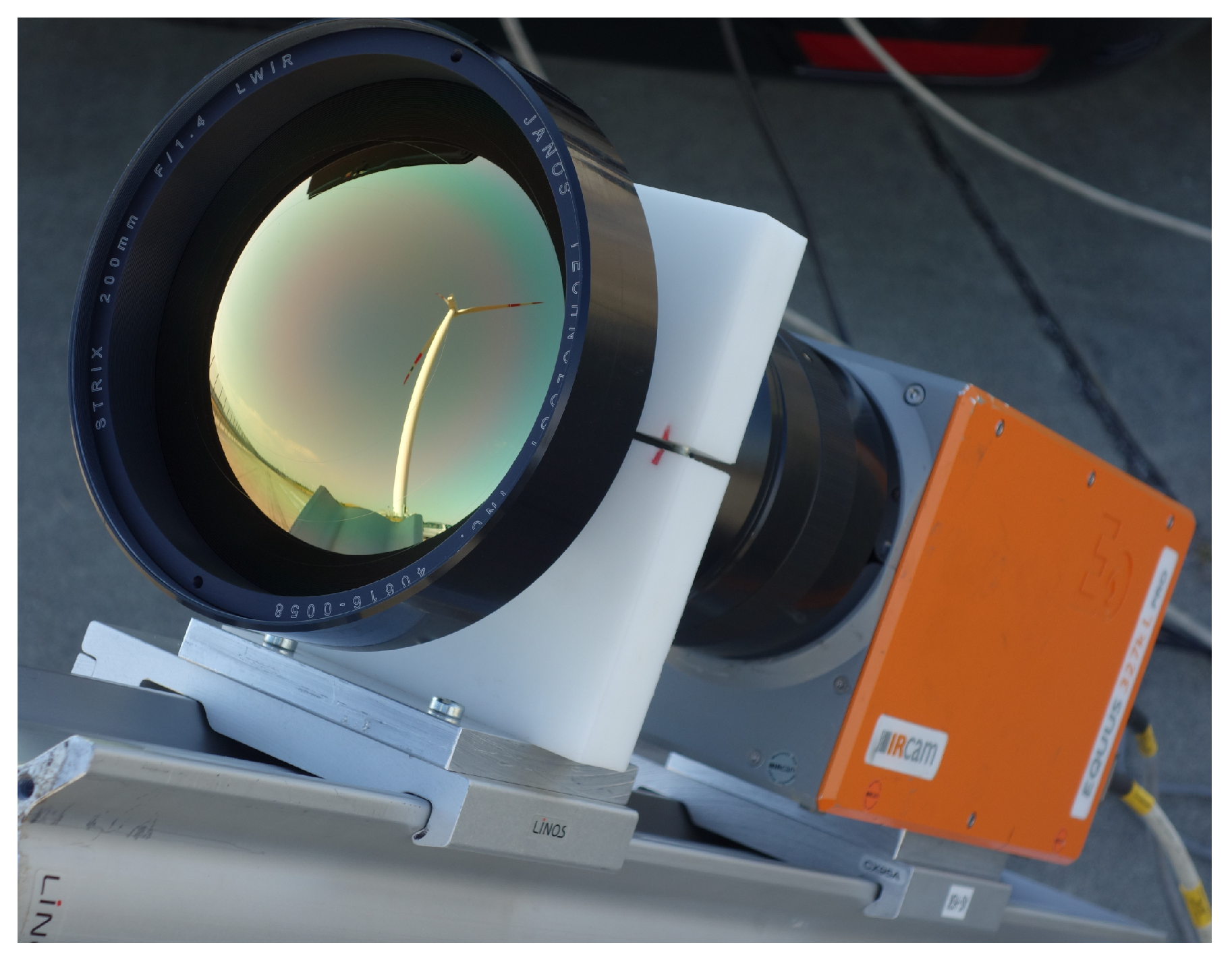
2.2.1. Thermographic Setup Provided by BIMAQ and DWGE
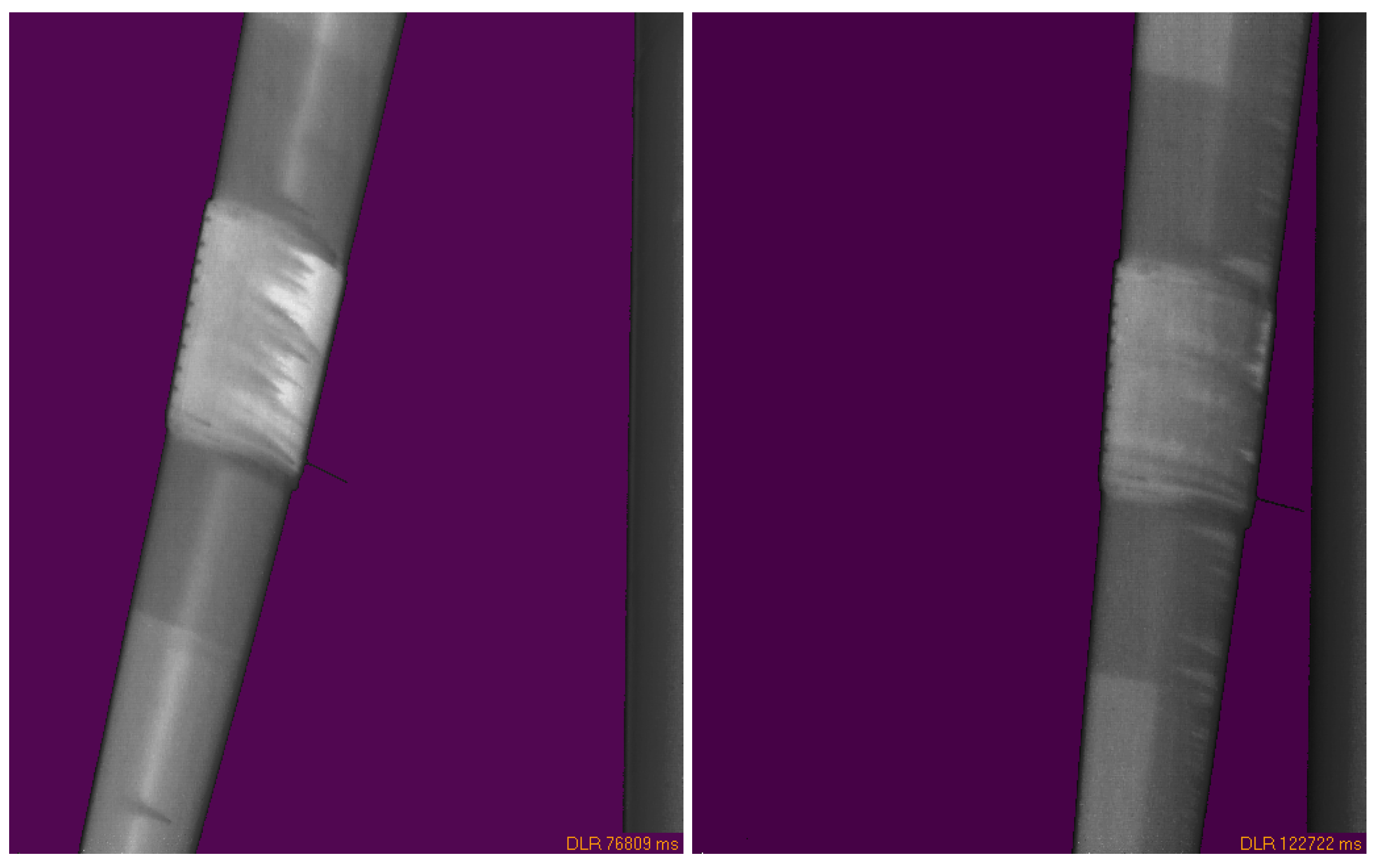
2.2.2. Thermographic Setup Provided by DLR
2.3. Optical Camera
3. Computational Fluid Dynamics
3.1. Set-Up
- low: 996 k tests + 149 k prisms
- medium: 853 k tets + 149 k prisms
- high: 4158 k test + 1744 k prisms
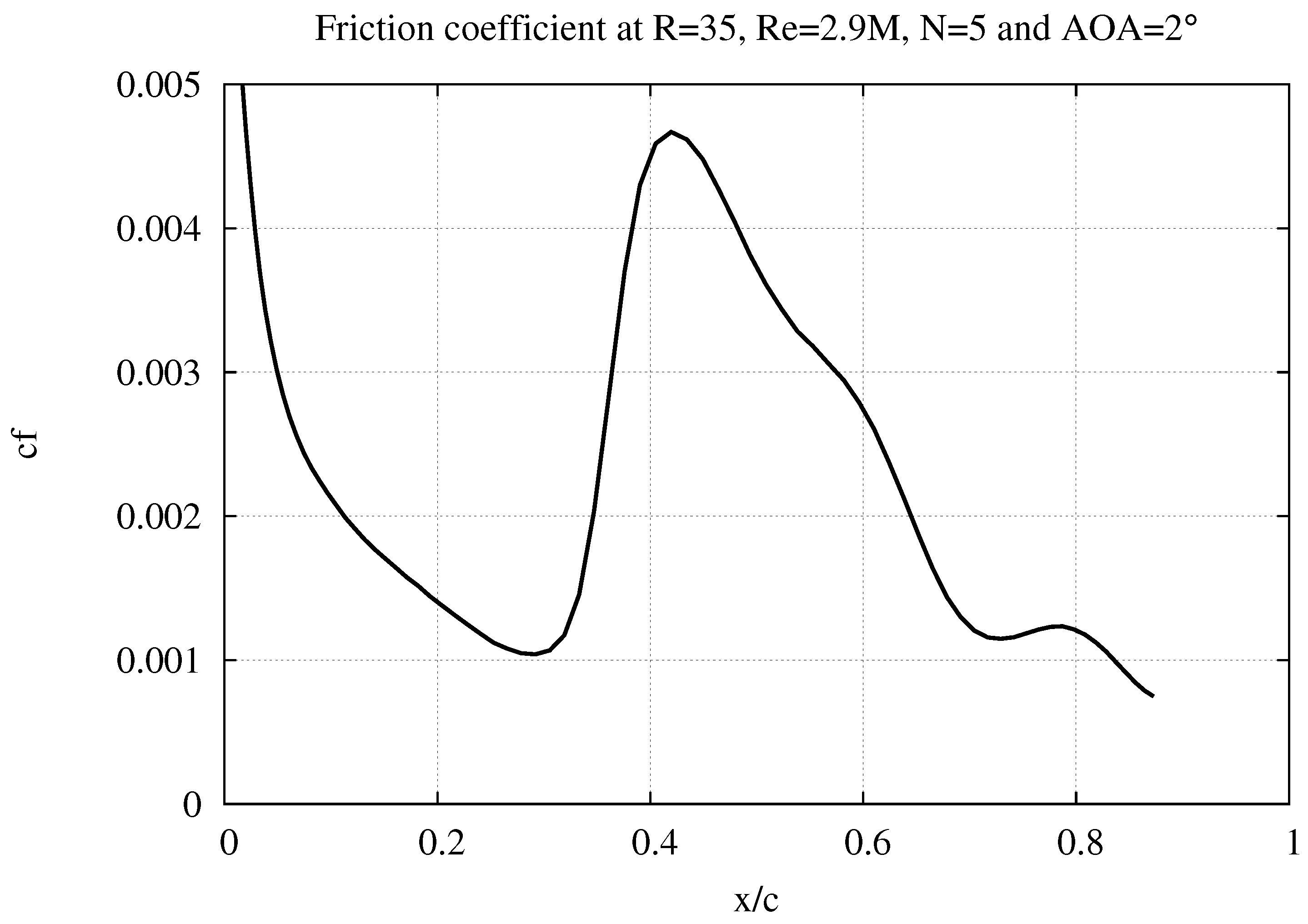
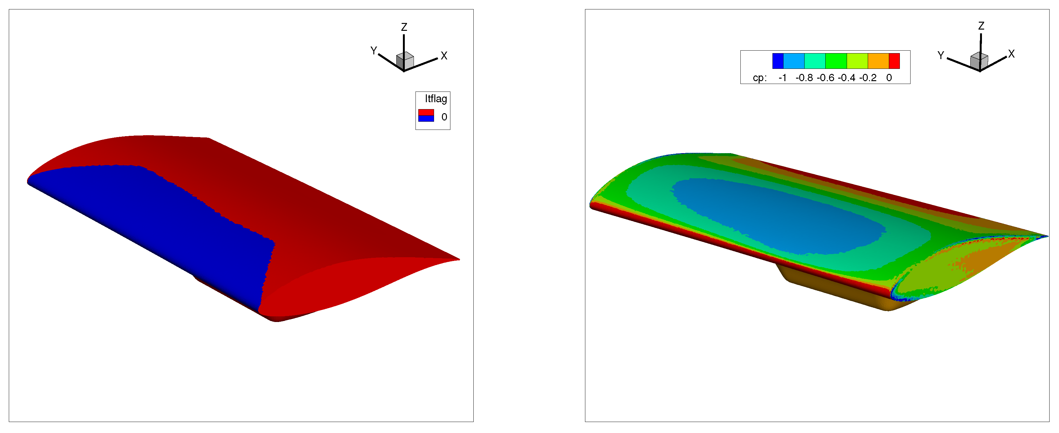
3.2. Results from CFD
4. Measurement Results
4.1. Measurements
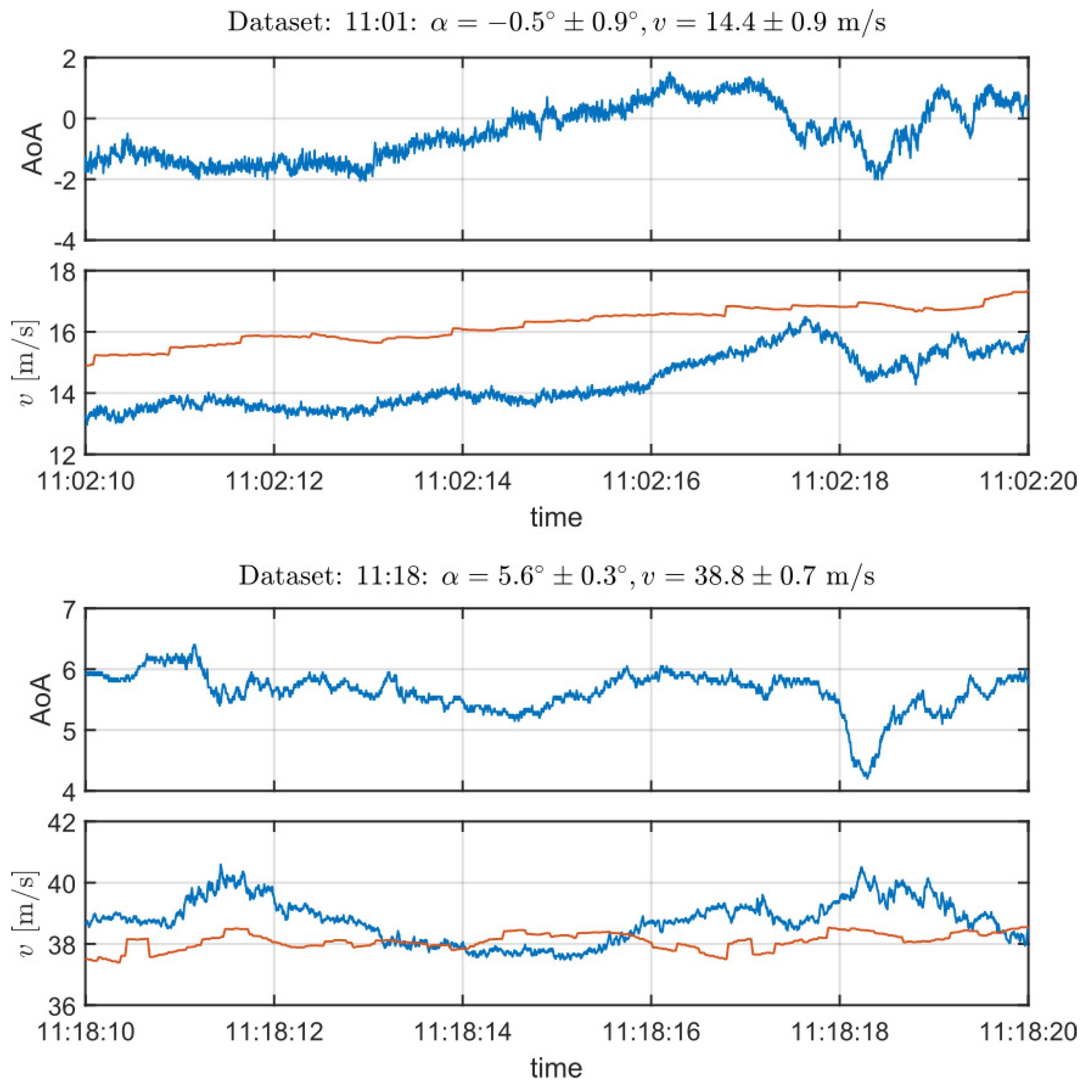
4.2. Inflow
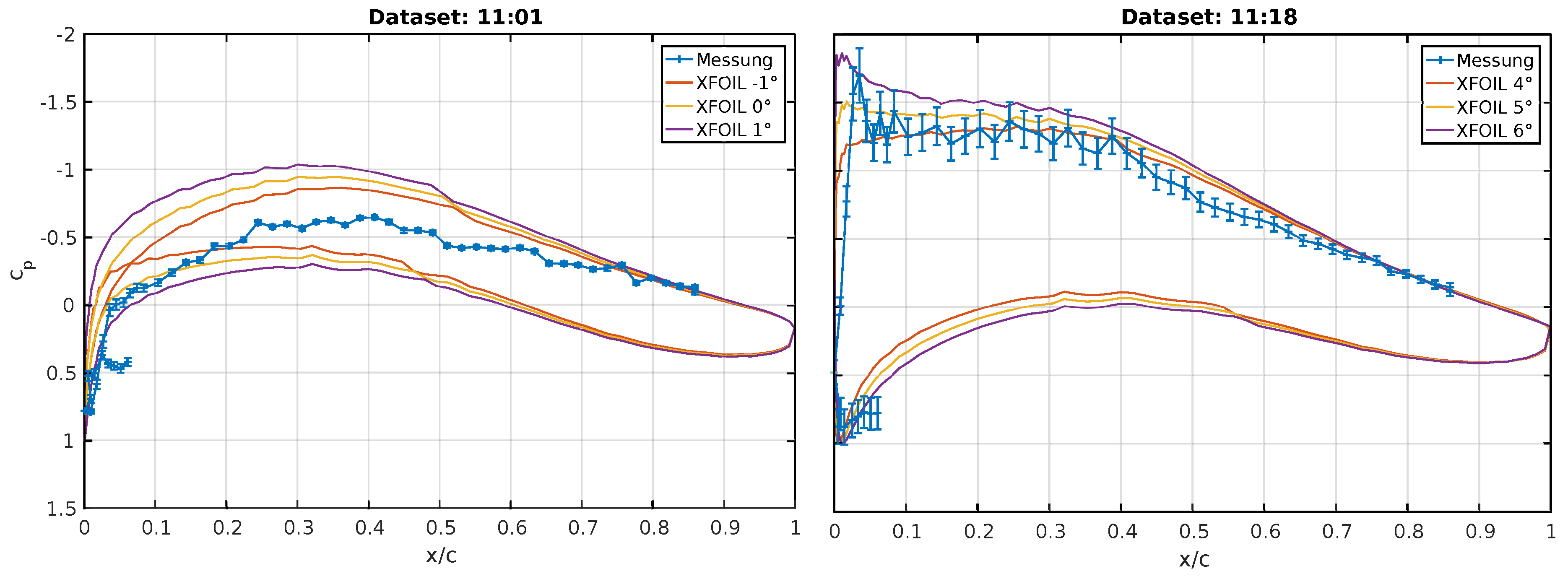
4.3. Pressure Distribution
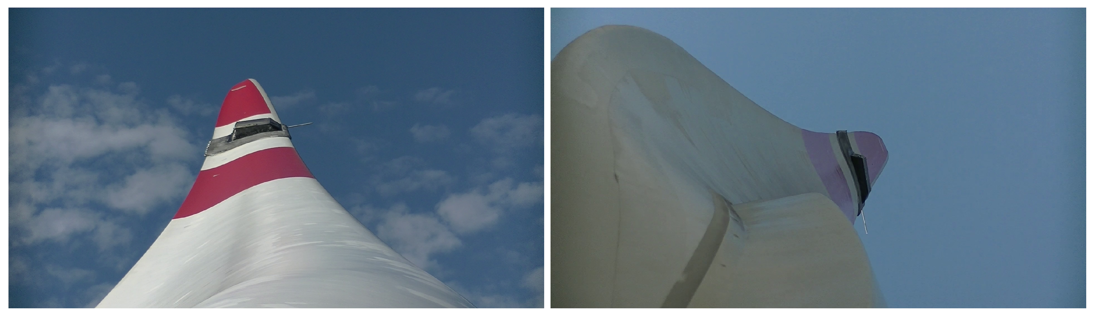
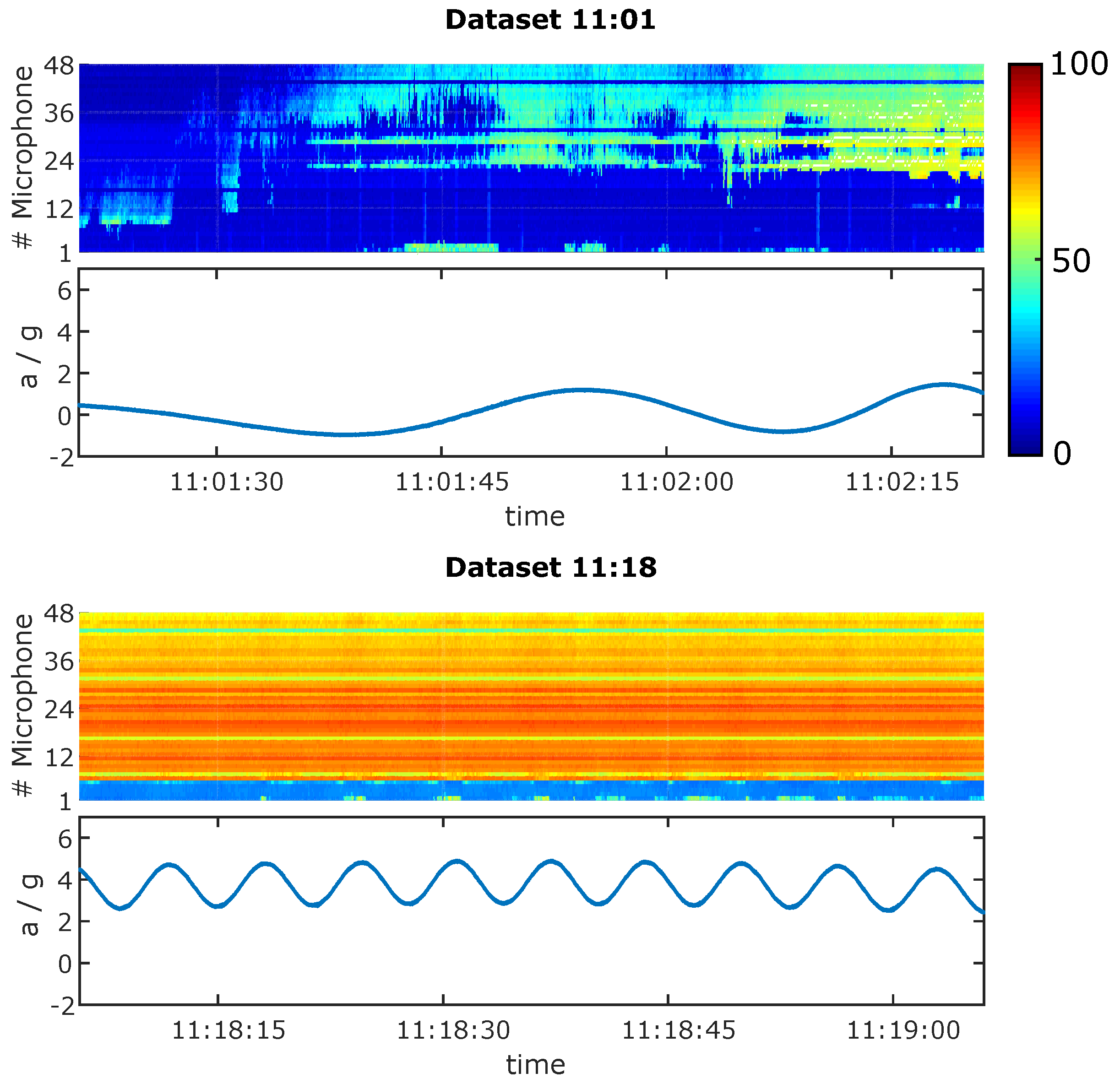
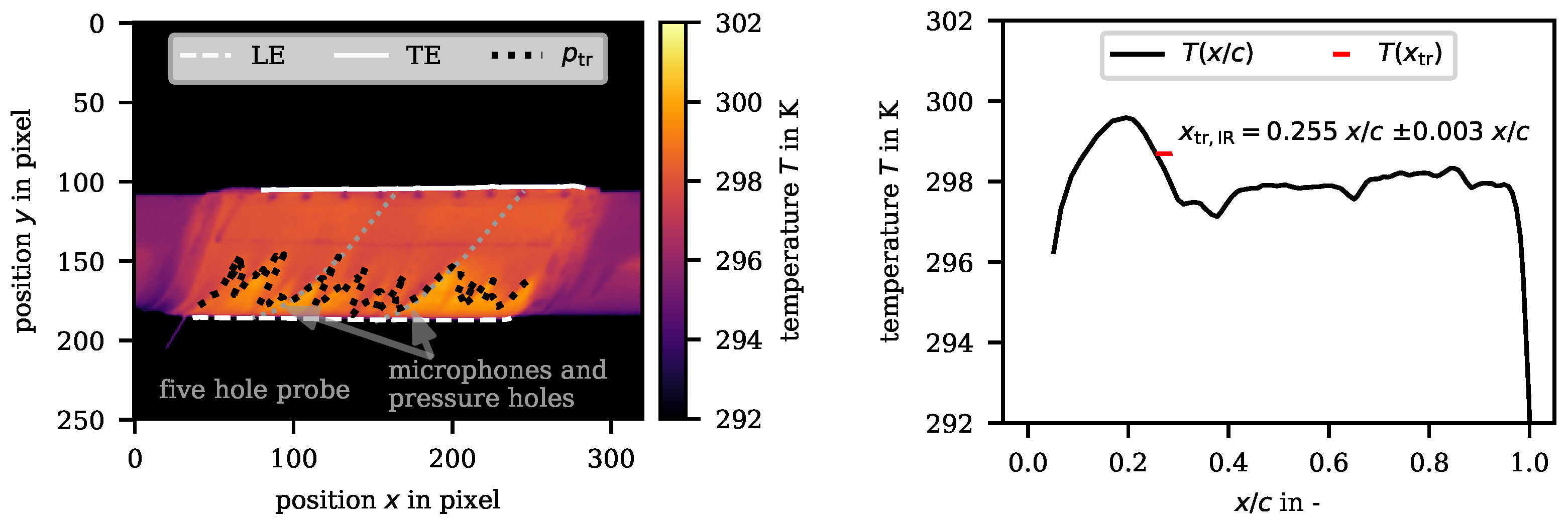
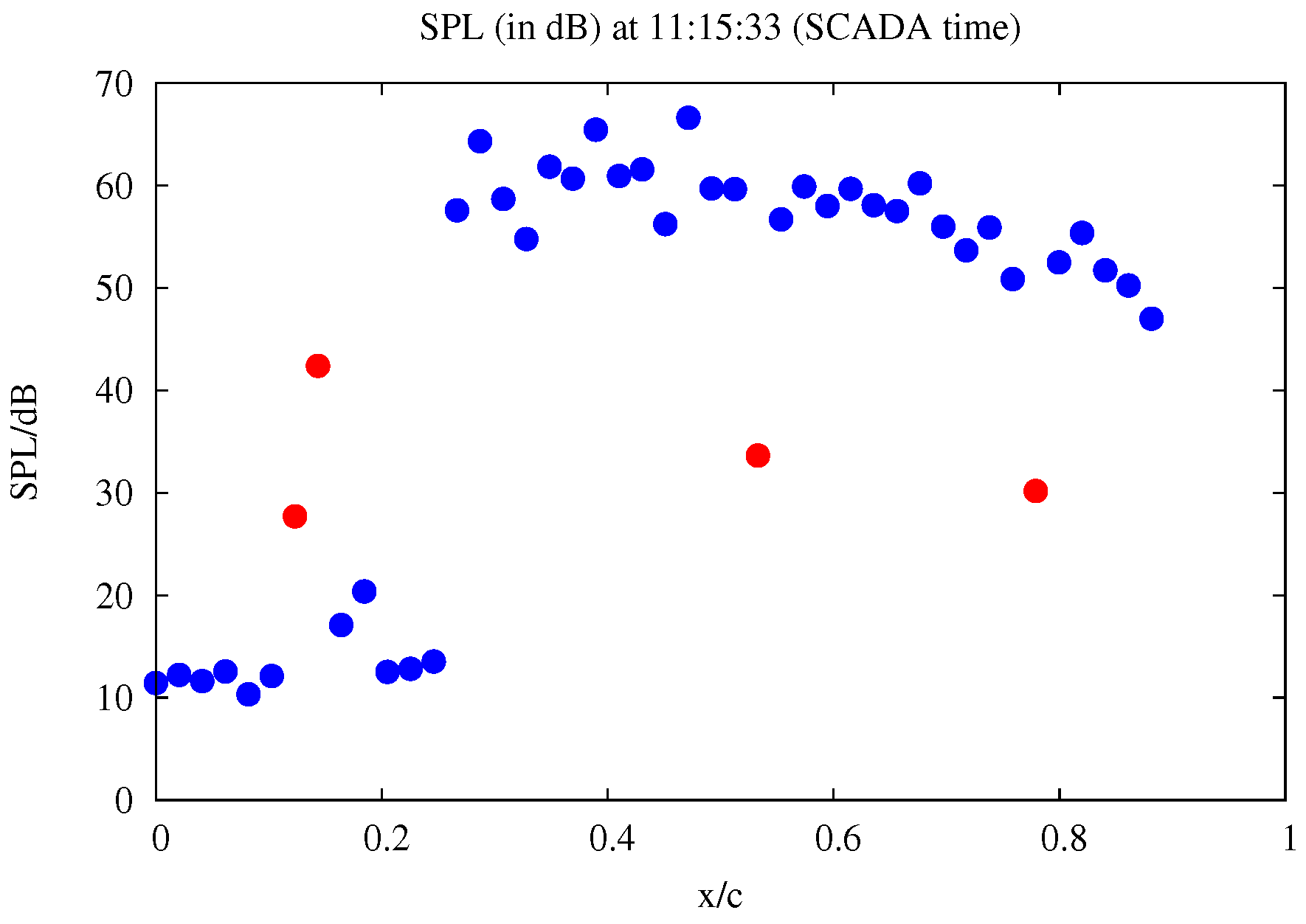
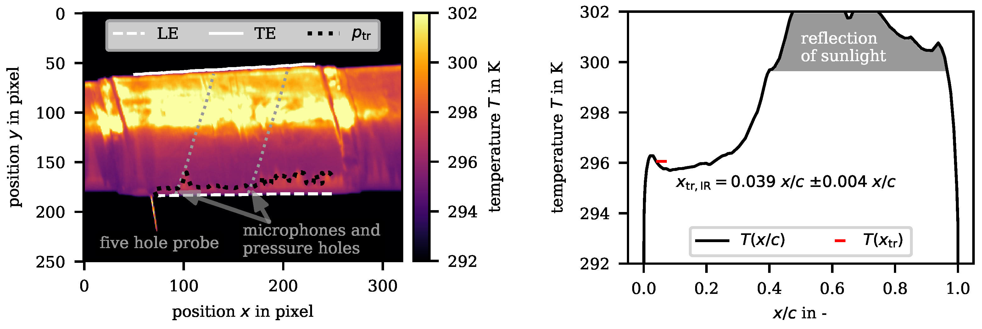
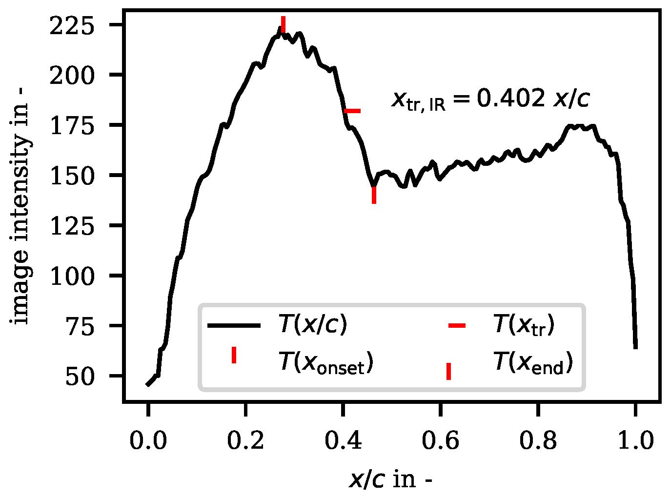
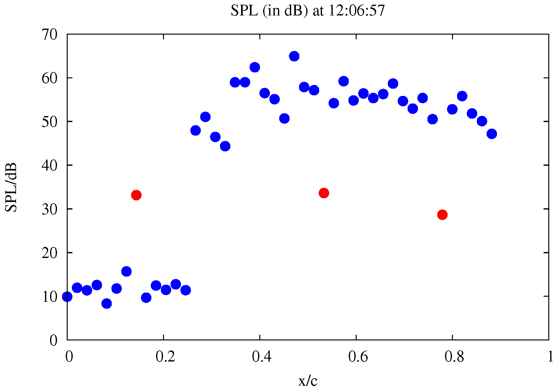
4.4. Detection of Transition Position
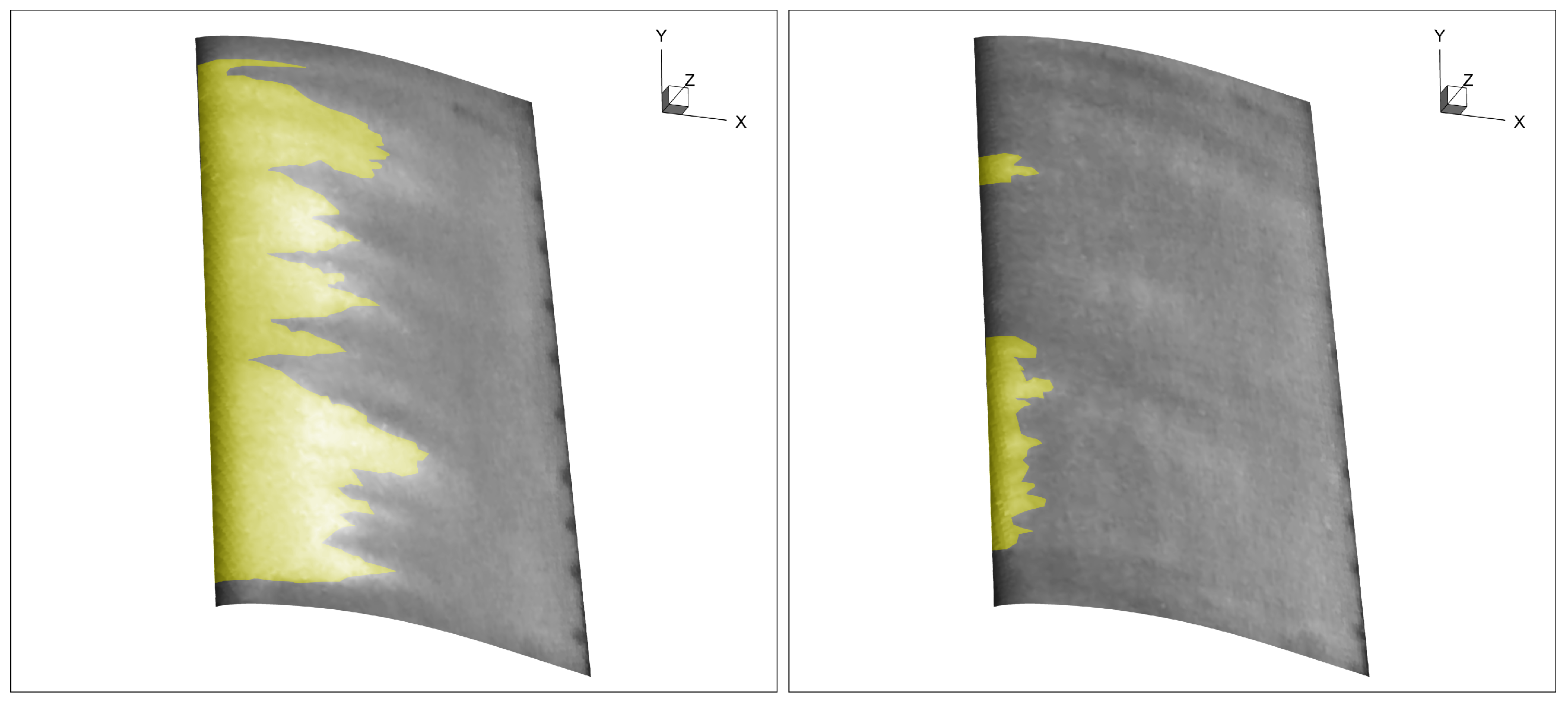
4.5. Thermography Team BIMAQ and DWGE
4.6. Results Team DLR
4.7. Discussion
5. Summary, Conclusions, and Future Research
- A new glove with a surface treatment in accordance at least with ordinary WT blades will be manufactured,
- microphones will be placed close to the tail to investigate noise emission,
- a small LIDAR device will be included into the glove,
- passive and active flow control devices will be investigated, and
- an LES (large Eddy Simulation) model will be developed with an inflow generator to simulated highly turbulent inflow to improve transition detection on WT blades by simulation.
Author Contributions
Funding
Acknowledgments
Conflicts of Interest
Abbreviations
| AOA | Angle of attack |
| BIMAQ | Bremer Institute for Metrology, Automation, and Quality Science |
| CFD | Computational Fluid Dynamics |
| DLR | German Aerospace Center |
| DTC | Digital Temperature Compensation |
| DWGE | Deutsche WindGuard Engineering GmbH |
| L2D | Lift-to-drag |
| SCADA | Supervisory Control and Data Acquisition |
| SPL | Sound-pressure level |
| SS | Steady-state phase |
| SSD | Solid-state disk |
| SU | Start-up phase |
| TI | Turbulence intensity |
| TSR | Tip-speed ratio |
| WT | Wind turbine |
References
- Schaffarczyk, A. (Ed.) Understanding Wind Power Technology; Wiley: Chichester, UK, 2014. [Google Scholar] [CrossRef]
- Schaffarczyk, A.P. Introduction to Wind Turbine Aerodynamics; Springer: Berlin, Germany, 2014. [Google Scholar]
- Abbot, I.H.; von Doenhoff, A. Theory of Wind Sections; Dover Publications Inc.: New York, NY, USA, 1959. [Google Scholar]
- Ceyhan, O.; Pires, O.; Munduate, X.; Sorensen, N.N.; Schaffarczyk, A.P.; Reichstein, T.; Diakakis, K.; Papadakis, G.; Daniele, E.; Schwarz, M.; et al. Summary of the Blind Test Campaign to predict the High Reynolds number performance of DU00-W-210 airfoil. In Proceedings of the AiAA SciTech Forum, Grapevine, TX, USA, 9–13 January 2017. [Google Scholar]
- TAU-Code User Guide, Release 2018.1.0; Technical Report; Deutsches Zentrum für Luft- und Raumfahrt e.V., Institute of Aerodynamics and Flow Technology: Göttingen, Germany, 2018.
- Seitz, A.; Horstmann, K.H. In-flight investigation of Tollmien-Schlichting waves. In IUTAM Symposium on One Hundret Years of Boundary Layer Research; Meier, G., Sreenivasan, K., Eds.; Springer: Dordrecht, The Netherlands, 2006; pp. 115–124. [Google Scholar]
- Reeh, A.; Tropea, C. Behaviour of a natural laminar flow airfoil in flight through atmospheric turbulence. J. Fluid Mech. 2015, 767, 394–429. [Google Scholar] [CrossRef]
- Van Groenewoud, G.J.H.; Boermans, L.M.M.; van Ingen, J.L. Onderzoek naar de Omslag Laminar-Turbulent van de Grensllag op de Rotorblades van de 25 m HAT Windturbine; Rapport LR-390; Technische Hogeschool Delft: Delft, The Netherlands, 1983. [Google Scholar]
- Van Ingen, J.L.; Schepers, J.G. Prediction of boundary layer transition on the wind turbine blades using th eN method and a comparison with experiment. Unpublished paper by private communication.
- Troldborg, N.; Bak, C.; Aagaard Madsen, H.; Skrzypinski, W. DANAERO MW: Final Report; DTU Wind Energy: Lyngby, Denmark, 2013. [Google Scholar]
- Madsen, H.; Fuglsang, P.; Romblad, J.; Enevoldsen, P.; Laursen, J.; Jensen, L.; Bak, C.; Paulsen, U.; Gaunaa, M.; Soerensen, N.N.; et al. The DAN-AERO MW Experiments. In Proceedings of the 48th AIAA Aerospace Science Meeting Including the New Horizons Forum and Aerospace Exposition, Aerospace Science Meetings, Orlando, FL, USA, 4–7 January 2010. [Google Scholar]
- Madsen, H.A.; Özçakman, Ö.S.; Bak, C.; Troldborg, N.; Sørensen, N.N.; Sørensen, J.N. Transition characteristics measuremd on a 2 MW 80 m diameter wind turbine rotor in comparison with transition data from wind tunnel measurements. In Proceedings of the AIAA Scitech Forum, San Diego, CA, USA, 7–11 January 2019. [Google Scholar]
- IEA Wind Task 29. Available online: https://community.ieawind.org/task29/home (accessed on 21 January 2019).
- Schwab, D.; Ingwersen, S.; Schaffarczyk, A.; Breuer, M. Aerodynamic Boundary Layer Investigation on a Wind Turbine Blade under Real Conditions. In Wind Energy—Impact of Turbulence; Hölling, M., Peinke, J., Ivanell, S., Eds.; Springer: Berlin/Heidelberg, Germany, 2014; pp. 203–208. [Google Scholar]
- Schaffarczyk, A.P.; Schwab, D.; Breuer, M. Experimental detection of laminar-turbulent transition on a rotating wind turbine blade in the free atmosphere. Wind Energy 2017, 20, 211–220. [Google Scholar] [CrossRef]
- Schwab, D. Aerodynamische Grenzschichtuntersuchungen an einem Windturbinenblatt im Feldversuch. Ph.D. Thesis, Helmut-Schmidt-Univesität, Universität der Bundeswehr Hamburg, Hamburg, Germany, 2018. (In German). [Google Scholar]
- Schaffarczyk, A.; Boisard, R.; Boorsma, K.; Dose, B.; Lienard, C.; Madsen, T.L.H.Å.; Rahimi, H.; Reichstein, T.; Schepers, G.; Sørensen, N.; et al. Comparison od 3D transitional CFD simulations for rotating wings with measurements. J. Phys. Conf. Ser. 2018. [Google Scholar] [CrossRef]
- Troen, I.; Lundtang Petersen, E. European Wind Atlas; Technical Report; Risø National Laboratory: Rosklilde, Denmark, 1989. [Google Scholar]
- Schaffarczyk, A.P.; Schwab, D.; Ingwersen, S.; Breuer, M. Pressure and hot-film measurements on a wind turbine blade operating in the atmosphere. J. Phys. Conf. Ser. 2014, 555, 012092. [Google Scholar] [CrossRef]
- de Luca, L.; Carlomagno, G.M.; Buresti, G. Boundary layer diagnostics by means of an infrared scanning radiometer. Exp. Fluids 1990, 9, 121–128. [Google Scholar] [CrossRef]
- Gartenberg, E.; Roberts, A.S. Airfoil transition and separation studies using an infrared imaging system. J. Aircraft 1991, 28, 225–230. [Google Scholar] [CrossRef]
- Dollinger, C.; Sorg, M.; Balaresque, N.; Fischer, A. Measurement uncertainty of IR thermographic flow visualization measurements for transition detection on wind turbines in operation. Exp. Ther. Fluid Sci. 2018, 97, 279–289. [Google Scholar] [CrossRef]
- Wolf, C.C.; Mertens, C.; Gardner, A.D.; Dollinger, C.; Fischer, A. Optimization of differential infrared thermography for unsteady boundary layer transition measurement. Exp. Fluids 2019, 60. [Google Scholar] [CrossRef]
- Dollinger, C.; Balaresque, N.; Sorg, M.; Fischer, A. IR thermographic visualization of flow separation in applications with low thermal contrast. Infrared Phys. Technol. 2018, 88, 254–264. [Google Scholar] [CrossRef]
- Gartenberg, E.; Roberts, A.S. Twenty-five years of aerodynamic research with infrared imaging. J. Aircraft 1992, 29, 161–171. [Google Scholar] [CrossRef]
- Joseph, L.A.; Borgoltz, A.; Devenport, W. Infrared thermography for detection of laminar-turbulent transition in low-speed wind tunnel testing. Exp. Fluids 2016, 57, 77. [Google Scholar] [CrossRef]
- Montelpare, S.; Ricci, R. A thermographic method to evaluate the local boundary layer separation phenomena on aerodynamic bodies operating at low Reynolds number. Int. J. Therm. Sci. 2004, 43, 315–329. [Google Scholar] [CrossRef]
- Crawford, B.K.; Duncan, G.T.; West, D.E.; Saric, W.S. Robust, automated processing of IR thermography for quantitative boundary-layer transition measurements. Exp. Fluids 2015, 56, 149. [Google Scholar] [CrossRef]
- Richter, K.; Schülein, E. Boundary-layer transition measurements on hovering helicopter rotors by infrared thermography. Exp. Fluids 2014, 55, 1755. [Google Scholar] [CrossRef]
- Dollinger, C.; Balaresque, N.; Gaudern, N.; Gleichauf, D.; Sorg, M.; Fischer, A. IR thermographic flow visualization for the quantification of boundary layer flow disturbances due to the leading edge condition. Renew. Energy 2019, 138, 709–721. [Google Scholar] [CrossRef]
- XFOIL v6.99. Available online: https://web.mit.edu/drela/Public/web/xfoil/ (accessed on 21 March 2019).
- Installation and User Manual of the FLOWer Main Version, Release 1-2008.1; Technical Report; Deutsches Zentrum für Luft- und Raumfahrt e.V., Institute of Aerodynamics and Flow Technology: Göttingen, Germany, 2008.
- Mack, L.M. Transition and Laminar Instability; Technical Report NASA-CP-153203; JPL-PUBL-77-15; Jet Propulsion Laboratory, California Institute of Technology: Pasadena, CA, USA, 1977. [Google Scholar]
- Mack, L.M. Boundary-Layer Linear Stability Theory; Technical Report 709; AGARD: Neuilly-sur-Seine, France, 1984. [Google Scholar]
- Schülein, E. Experimental Investigation of Laminar Flow Control on a Supersonic Swept Wing by Suction. In Proceedings of the AIAA-2008-4208, 4th Flow Control Conference, Seattle, WA, USA, 23–26 June 2008. [Google Scholar]


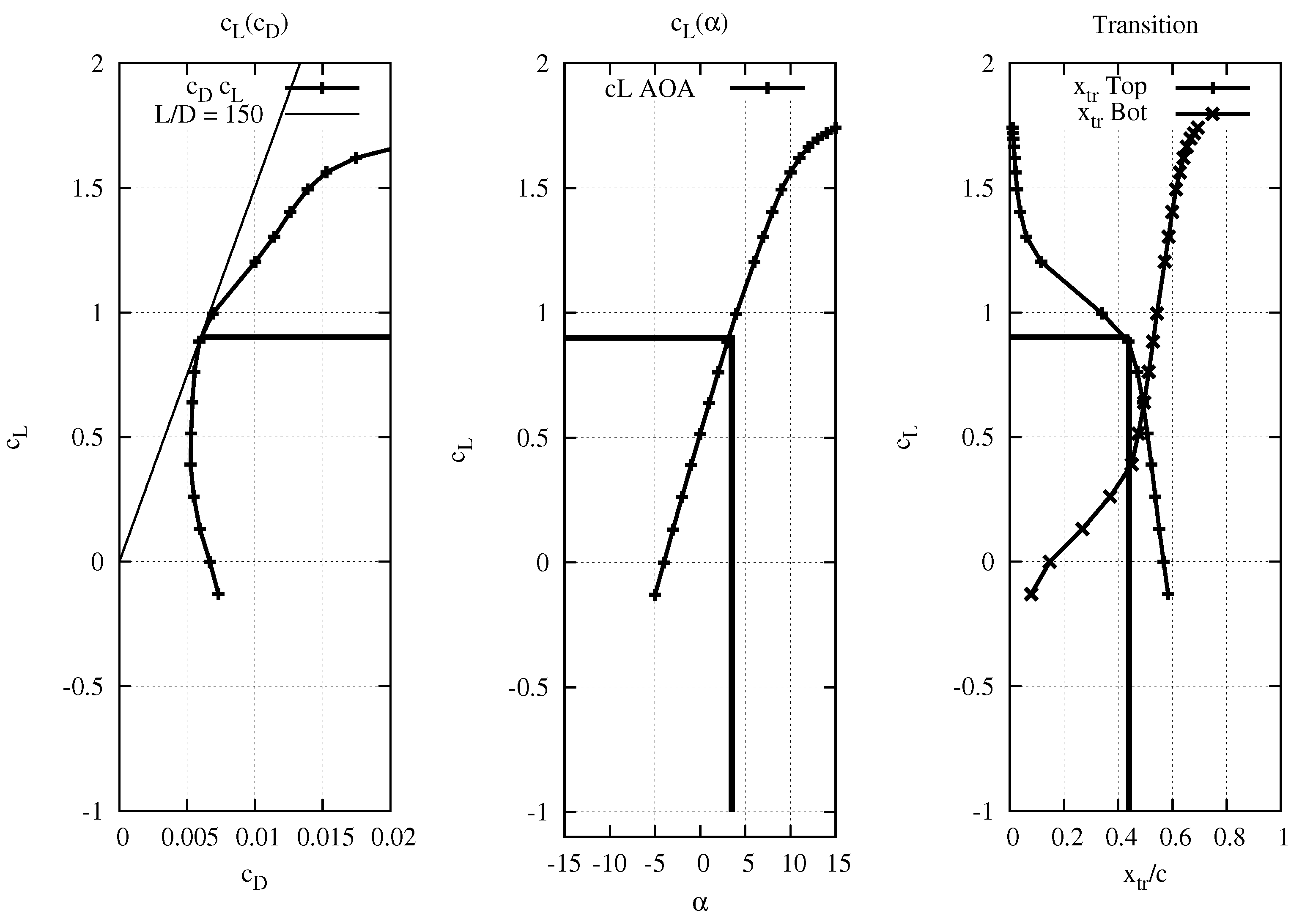
| Quantity | Value | Unit |
| 0.9 | - | |
| 0.005 | - | |
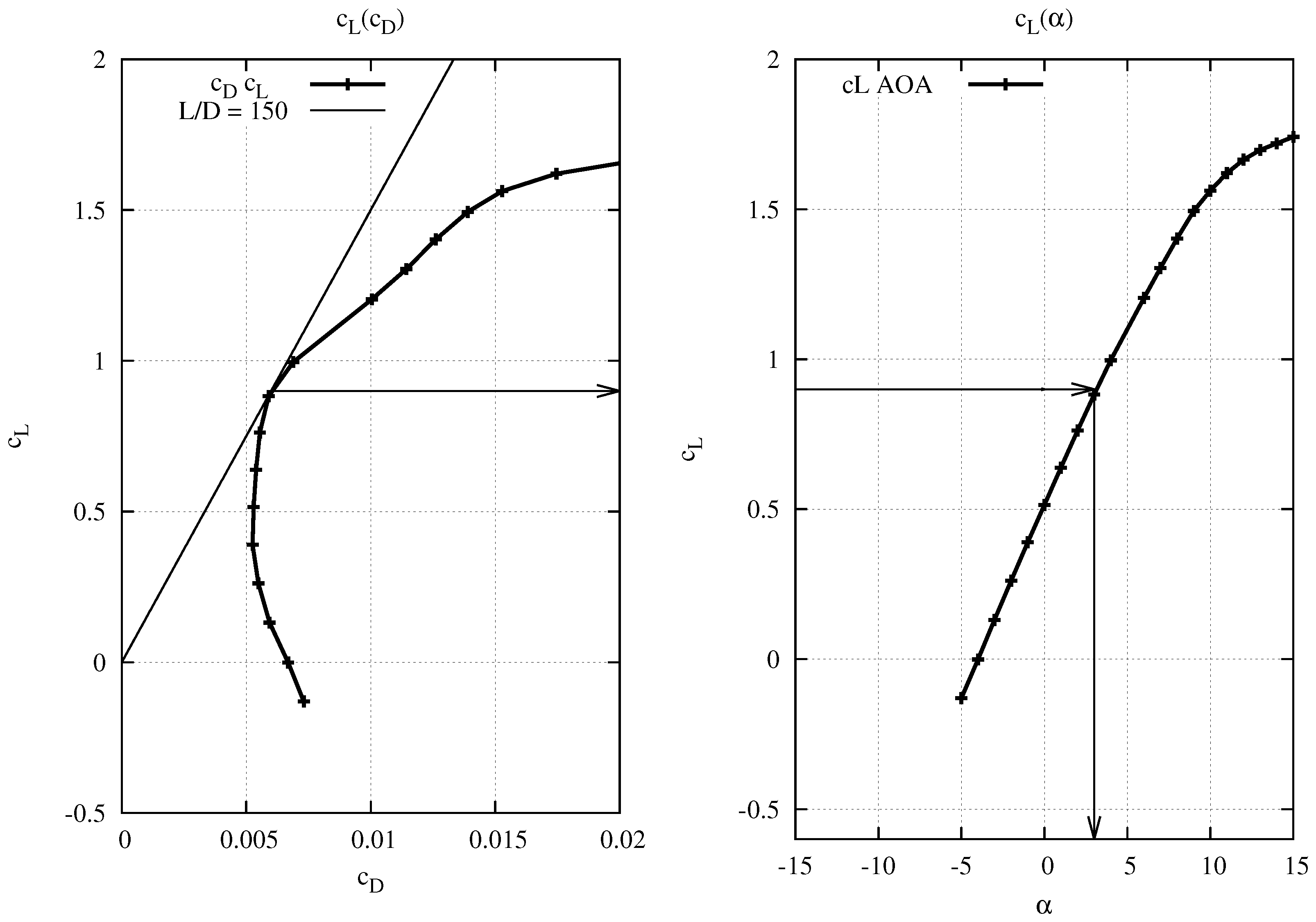
| Maximum lift over drag (L2D) | 150 | - |
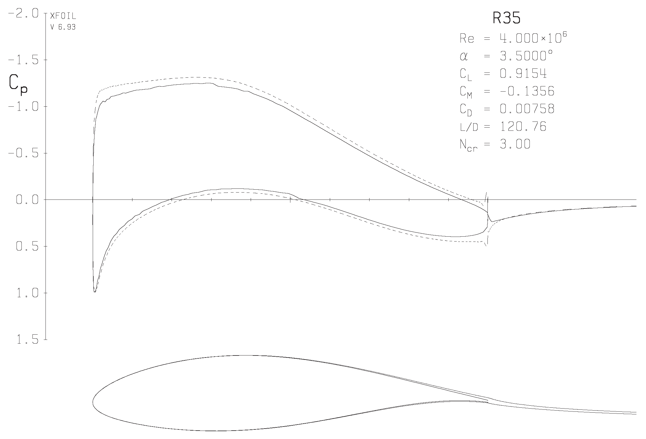
| Angle of attack | 3.5 | deg |
| Laminar part (suction or top side) | 0.45 |
© 2019 by the authors. Licensee MDPI, Basel, Switzerland. This article is an open access article distributed under the terms and conditions of the Creative Commons Attribution (CC BY) license (http://creativecommons.org/licenses/by/4.0/).
Share and Cite
Reichstein, T.; Schaffarczyk, A.P.; Dollinger, C.; Balaresque, N.; Schülein, E.; Jauch, C.; Fischer, A. Investigation of Laminar–Turbulent Transition on a Rotating Wind-Turbine Blade of Multimegawatt Class with Thermography and Microphone Array. Energies 2019, 12, 2102. https://doi.org/10.3390/en12112102
Reichstein T, Schaffarczyk AP, Dollinger C, Balaresque N, Schülein E, Jauch C, Fischer A. Investigation of Laminar–Turbulent Transition on a Rotating Wind-Turbine Blade of Multimegawatt Class with Thermography and Microphone Array. Energies. 2019; 12(11):2102. https://doi.org/10.3390/en12112102
Chicago/Turabian StyleReichstein, Torben, Alois Peter Schaffarczyk, Christoph Dollinger, Nicolas Balaresque, Erich Schülein, Clemens Jauch, and Andreas Fischer. 2019. "Investigation of Laminar–Turbulent Transition on a Rotating Wind-Turbine Blade of Multimegawatt Class with Thermography and Microphone Array" Energies 12, no. 11: 2102. https://doi.org/10.3390/en12112102
APA StyleReichstein, T., Schaffarczyk, A. P., Dollinger, C., Balaresque, N., Schülein, E., Jauch, C., & Fischer, A. (2019). Investigation of Laminar–Turbulent Transition on a Rotating Wind-Turbine Blade of Multimegawatt Class with Thermography and Microphone Array. Energies, 12(11), 2102. https://doi.org/10.3390/en12112102